Variable Selection for Generalized Linear Mixed Models by L1-Penalized Estimation

Gerhard Tutz & Andreas Groll

Variable Selection for Generalized Linear Mixed

Models by

L

₁

-Penalized Estimation

Technical Report Number 108, 2011

Department of Statistics

University of Munich

Variable Selection for Generalized Linear Mixed Models

by

L

1

-Penalized Estimation

Andreas Groll

Gerhard Tutz

June 3, 2011

Abstract

Generalized linear mixed models are a widely used tool for modeling longitudinal data. How-ever, their use is typically restricted to few covariates, because the presence of many predictors yields unstable estimates. The presented approach to the fitting of generalized linear mixed models includes anL1-penalty term that enforces variable selection and shrinkage

simultane-ously. A gradient ascent algorithm is proposed that allows to maximize the penalized log-likelihood yielding models with reduced complexity. In contrast to common procedures it can be used in high-dimensional settings where a large number of potentially influential explana-tory variables is available. The method is investigated in simulation studies and illustrated by use of real data sets.

Keywords: Generalized linear mixed model, Lasso, Gradient ascent, Penalty, Linear models,

Variable selection

∗_{Department of Statistics, University of Munich, Akademiestrasse 1, D-80799, Munich, Germany, email:} [email protected]

†_{Department of Statistics, University of Munich, Akademiestrasse 1, D-80799, Munich, Germany, email:} [email protected]

1

Introduction

Generalized linear mixed models (GLMMs) are widely used to model correlated and clustered responses. Various estimation methods have been proposed ranging from numerical integration techniques (for example Booth and Hobert, 1999) over “joint maximization methods” (Breslow and Clayton, 1993; Schall, 1991), in which parameters and random effects are estimated si-multaneously, to fully Bayesian approaches (Fahrmeir and Lang, 1999). Overviews on current methods are found in McCulloch and Searle (2001). Due to the heavy computational problems in GLMMs modeling usually is restricted to few predictor variables. When many predictors are available, estimates become very unstable. Therefore, procedures to select the relevant vari-ables are important in modelling. Classical approaches to the selection of predictors are based on test statistics with the usual stability problems of forward-backward algorithms, which are due to the inherent discreteness of the method (for example Breiman, 1996).

A more timely approach to variable selection is based on boosting methods, which have originally been developed within the machine learning community as a method to improve classification. A first breakthrough was the AdaBoost algorithm proposed by Freund and Schapire (1996). Breiman (1998) considered the AdaBoost algorithm as a gradient descent optimization technique and Friedman (2001) extended boosting methods to include regression problems. B¨uhlmann and Yu (2003) showed how to fit smoothing splines by boosting base learners and introduced the concept of componentwise boosting, which may be exploited to select predictors. For a detailed overview of componentwise boosting, see B¨uhlmann and Yu (2003) and B¨uhlmann and Hothorn (2007). For linear mixed models the incorporation of random effects has been considered by Tutz and Reithinger (2007), first attempts to fit univariate GLMMs were proposed by Tutz and Groll (2010).

An alternative approach to variable selection that has received much attention is based on penalized regression techniques. The Lasso proposed by Tibshirani (1996) has become a very popular approach to regression that uses anL1-penalty on the regression coefficients. This has

the effect that all coefficients are shrunken towards zero and some are set exactly to zero. The basic idea is to maximize the log-likelihoodl(βββ) of the model while constraining the L1-norm

of the parameter vectorβββ. Thus one obtains the Lasso estimate ˆ β β β = argmax βββ l(βββ), subject to ||βββ||1≤s, (1)

derived by solving the optimization problem ˆ β β β = argmax βββ [l(βββ)−λ||βββ||1], (2)

with λ ≥ 0. Both s and λ are tuning parameters that have to be determined, for example by cross-validation. This can be very time-consuming, especially in high-dimensional data settings. Thus, to get computation time under control, in general problems that involve a complex log-likelihood, efficient algorithms are needed to derive the solutions of equations (1) or (2).

Forlinear models the optimization problem of the Lasso can be solved by quadratic

pro-gramming (Tibshirani, 1996), whereas Osborne et al. (2000) recommend an algorithm con-sidering simultaneously the primal problem and its dual, which is highly efficient and is also applicable in high-dimensional cases. A substantial progress was achieved by the LARS algo-rithm (Efron et al., 2004), which simultaneously produces the set of Lasso fits for all values of the tuning parameters by following the exact, piecewise linear solution path ofβββ as a function ofsorλ, respectively, and also inspired the regularization path algorithm for the support vec-tor machine (Hastie et al., 2004). In the last decade several improvements have been designed for the Lasso, e.g. the adaptive Lasso (Zou and Hastie, 2006), SCAD (Fan and Li, 2001), the Elastic Net (Zou and Hastie, 2005), the Dantzig selector (Candes and Tao, 2007), the Double Dantzig (James and Radchenko, 2009) and the VISA (Radchenko and James, 2008).

The Lasso has been extended to more general models, for example Tibshirani (1997) pro-posed a new method to perform variable selection in the Cox model. He minimizes the partial log-likelihood subject to theL1-norm of the parameters being bounded by a constant, which is

done by an iterative two-step estimation scheme, using alternately reweighted least squares and adaption to the constraint through a quadratic programming procedure. This procedure was improved by Gui and Li (2005), who suggested an iteratively reweighted estimation approach based on the LARS algorithm, called the LARS-Cox procedure. But according to Segal (2006) and Goeman (2010) both algorithms are computational so demanding, that they cannot be used very well in high-dimensional scenarios.

For generalized linear models a flexible and efficient approach is the L1-regularized path

following algorithm by Park and Hastie (2007), who extended the concept of the LARS al-gorithm (Efron et al., 2004) to generalized linear models. The exact solution coefficients ˆβj

are computed at particular values of the smoothing parameterλand then the coefficients are connected in a piecewise linear manner. Another promising approach uses the componentwise gradients, initiating from a starting valueβββ(0)and then running through the single coordinates ofβββ, updating them accordant to the gradient of the penalized likelihood (see e.g. Shevade

and Keerthi, 2003, Kim and Kim, 2004 or Genkin et al., 2007). Recently Goeman (2010) presented another approach based on a combination of gradient ascent optimization with the Newton-Raphson algorithm.

The use of penalization techniques for the selection of variables in mixed models is still in the beginning. For Gaussian mixed models Ni et al. (2010) proposed SCAD penalty techniques. Bondell et al. (2010) considered the iterative case of joint selection for fixed and random effects in linear models. In the following we developL1-penalty approaches for the generalized linear

mixed model. The method works by combining gradient ascent optimization with the Fisher scoring algorithm and is based on the approach of Goeman (2010). The article is structured as follows. In Section 2 we introduce the GLMM. In Section 3 we present the gradient ascent algorithm with its computational details and give further information about starting values and computation of tuning parameters. Then the performance of the gradient ascent algorithm is investigated in two simulation studies. Applications are considered in Section 4.

2

Generalized Linear Mixed Models - GLMMs

Let yit denote observation t in cluster i, i = 1, . . . , n, t = 1, . . . , Ti, collected in yTi =

(yi1, . . . , yiTi). Letx

T

it= (1, xit1, . . . , xitp) be the covariate vector associated with fixed effects

andzT

it= (zit1, . . . , zitq) be the covariate vector associated with random effects. It is assumed

that the observations yit are conditionally independent with means µit = E(yit|bi,xit,zit)

and variancesvar(yit|bi) =φυ(µit), whereυ(.) is a known variance function and φis a scale

parameter. The GLMM that we consider in the following has the form

g(µit) =xTitβββ+zTitbi=ηitpar+η

rand

it , (3)

where g is a monotonic and continuously differentiable link function, ηpar

it = xTitβββ is a linear

parametric term with parameter vectorβββT = (β0, β1, . . . , βp) including intercept and ηitrand = zT

itbi contains the cluster-specific random effects bi ∼N(0,Q), withq×q covariance matrix Q. An alternative form that we also use is

µit=h(ηit), ηit=β0+ηitpar+η

rand

it ,

whereh=g−1 _{is the inverse link function.}

A closed representation of model (3) is obtained by using matrix notation. By collecting observations within one cluster, the model has the form

whereXTi = (xi1, . . . ,xiTi) denotes the design matrix of thei-th cluster andZ

T

i = (zi1, . . . ,ziTi).

For all observations one obtains

g(µµµ) =Xβββ+Zb, with XT = [XT1, . . . ,X

T

n] and block-diagonal matrix Z = Blockdiag(Z1, . . . ,Zn). For the

random effects vector bT = (bT1, . . . ,b T

n) one has a normal distribution with block-diagonal

covariance matrixQb=diag(Q, . . . ,Q).

Focusing on GLMMs we assume that the conditional density of yit, given explanatory

variables and the random effectbi, is of exponential family type

f(yit|xit,bi) = exp _(y itθit−κ(θit)) φ +c(yit, φ) ,

where θit =θ(µit) denotes the natural parameter, κ(θit) is a specific function corresponding

to the type of exponential family, c(.) the log normalization constant and φ the dispersion parameter (compare Fahrmeir and Tutz, 2001).

One popular method to maximize GLMMs is penalized quasi-likelihood (PQL), which has been suggested by Breslow and Clayton (1993), Lin and Breslow (1996) and Breslow and Lin (1995). Typically the covariance matrixQ(%%%) of the random effectsbidepends on an unknown

parameter vector%%%. In penalization-based concepts the joint likelihood-function is specified by the parameter vector of the covariance structure%%%together with the dispersion parameter φ, which are collected inγγγT _{= (φ, %%%}T_{), and parameter vectorδδδ}T _{= (βββ}T

,bT). The corresponding log-likelihood is l(δδδ, γγγ) = n X i=1 log Z f(yi|δδδ, γγγ)p(bi, γγγ)dbi , (4)

wherep(bi, γγγ) denotes the density of the random effects. Breslow and Clayton (1993) derived

the approximation lapp_{(δδδ, γγγ) =} n X i=1 log(f(yi|δδδ, γγγ))− 1 2b T_Q(%%%)−1_{b, (5)}

where the penalty termbTQ(%%%)−1_{bis due to the approximation based on the Laplace method.}

PQL usually works within the profile likelihood concept. It is distinguished between the estimation ofδδδ, given the plugged-in estimate ˆγγγ, resulting in the profile-likelihood lapp_{(δδδ,γγγ),ˆ}

and the estimation ofγγγ. The PQL method is implemented in the macro GLIMMIX and proc GLMMIXin SAS (Wolfinger, 1994), in theglmmPQLandgamm functions of the R-packagesMASS (Venables and Ripley, 2002) and mgcv(Wood, 2006). Further notes were given by Wolfinger and O’Connell (1993), Littell et al. (1996) and Vonesh (1996).

3

Regularization in GLMMs

In the following the log-likelihood (4) is expanded to include the penalty term λPp_i=1|βi|.

Approximation along the lines of Breslow and Clayton (1993) yields the penalized log-likelihood

lpen_{(βββ,b, γγγ) =l}pen_{(δδδ, γγγ) =l}app_{(δδδ, γγγ)}

−λ

p

X

i=1

|βi|. (6)

For given ˆγγγ the optimization problem reduces to

ˆ δδδ= argmax δδδ lpen (δδδ,γγγ) = argmaxˆ δδδ " lapp (δδδ,γγγˆ)₋λ p X i=1 |βi| # . (7)

We will use a full gradient algorithm that is based on the algorithm of Goeman (2010). As Goeman (2010) already pointed out, the algorithm can easily be amended to situations in which some parameters should not be penalized. In this case the penalty term from the optimization problem of equation (2) is replaced by Pp_i=1λi|βi|, where λi = 0 is chosen for unpenalized

parameters. The penalty used in (6) and (7) can be seen as a partially penalized approach if the whole parameter vectorδδδT _{= (βββ}T

,bT) is considered.

3.1

Gradient Ascent Algorithm - glmmLasso

In the following an algorithm is presented for maximizing the penalized log-likelihoodlpen_{(δδδ, γγγ)}

from equation (6). In contrast to the approaches of Shevade and Keerthi (2003), Kim and Kim (2004) and Genkin et al. (2007), where only a single component is updated at a time, it follows the gradient of the likelihood from a given starting value ofδδδ and uses the full gradient at each step. Similar to Goeman (2010) the algorithm can automatically switch to a Fisher scoring procedure when it gets close to the optimum and therefore avoids the tendency to slow convergence which is typical for gradient ascent algorithms. An additional step is needed to estimate the variance-covariance componentsQ of the random effects. To keep the notation simple, we omit the argumentγγγ in the following description of the algorithm and writelapp_(δδδ)

instead oflapp_{(δδδ, γγγ).}

Algorithm glmmLasso

1. Initialization

Compute starting values ˆβββ(0),bˆ(0),γγγˆ(0)(see Section 3.2.1) and set ˆηηη(0) =Xβββˆ(0)+Zbˆ(0).

Forl= 1,2, . . .until convergence:

(a) Calculation of the log-likelihood gradient for givenγγγˆ(l−1)

Withs(δδδ) =∂lapp_{(δδδ)/∂δδδ derive:}

spen 0 (ˆδδδ (l−1) ) =s0(ˆδδδ (l−1) ), spen i (ˆδδδ (l−1) ) =si(ˆδδδ (l−1) ), i=p+ 1, . . . , p+ns.

Furthermore, fori= 1, . . . , pderive:

spen i (ˆδδδ (l−1) ) =          si(ˆδδδ (l−1) )−λsign ( ˆβi(l−1)) if ˆβ (l−1) i 6= 0 si(ˆδδδ (l−1) )−λsign (si(ˆδδδ (l−1) )) if ˆβi(l−1)= 0 and |si(ˆδδδ (l−1) )|> λ 0 otherwise , where sign(x) =          1 if x >0 0 if x= 0 −1 if x <0.

(b) Calculation of the dircetional second derivative

LetA:= [X,Z] andK=diag(0, . . . ,0,Q−1, . . . ,Q−1) be a block-diagonal penalty matrix with a diagonal ofp+ 1 zeros corresponding to the fixed effects and thenn times the matrixQ−1. Then the Fisher matrix is given in closed form asFpen

(δδδ) =

ATW(δδδ)A+K, with W(δδδ) = D(δδδ)ΣΣΣ−1_{(δδδ)D(δδδ)}T _{and D(δδδ) = ∂h(ηηη)/∂ηηη,ΣΣΣ(δδδ) =}

cov(y|δδδ). The directional second derivative is given for everyδδδ and every direction vectorv∈Rp+1+ns _by

lpen00 (δδδ;v) =v

T_Fpen_(δδδ)v

(c) Optimum of Taylor approximation

Based on the Taylor approximation used in Goeman (2010), we derive

t(edgel−1)= min i   − ˆ δi(l−1) spen i (ˆδδδ (l−1) )

: sign(ˆδ_i(l−1)) =₋sign[spen

i (ˆδδδ (l−1) )]₆= 0    and t(optl−1)= ||spen_(ˆδδδ(l−1)₎ ||2 l00 app(ˆδδδ (l−1) ,spen_(ˆδδδ(l−1)₎₎ , with_{|| · ||}2 denoting theL2 norm.

(d) Update ˆ δδδ(l)=              ˆ δδδ(l−1)+t(edgel−1)spen(ˆδδδ (l−1) ) if t(optl−1)≥t (l−1) edge ˆ δδδ(NRl−1) if t (l−1) opt < t (l−1)

edge and sign(ˆδδδ

(l) NR) = sign(ˆδδδ (l−1) ) ˆ δδδ(l−1)+t(optl−1)spen(ˆδδδ (l−1) ) otherwise,

where ˆδδδ(NRl) denotes the Fisher scoring estimate as given in Section 3.2.2.

(e) Computation of variance-covariance components

Estimates ˆQ(l) are obtained as approximate EM-type estimates or by alternative methods (see Section 3.2.3) yielding the update%%%(l)_{. If necessary, the whole vector}

ˆ

γγγ(l)is completed by an estimate of the dispersion parameter.

3. Re-Estimation

In a final step a model that includes only the variables corresponding to non-zero pa-rameters of ˆβββ is fitted. A simple Fisher scoring, resulting in the final estimates ˆδδδ,Qˆ is used.

3.2

Computational Details of

glmmLasso

In the following we give a more detailed description of the single steps of the glmmLasso algorithm. First details of the computation of starting values are given and then two estimation techniques for the variance-covariance components are described.

3.2.1 Starting Values forglmmLasso

We compute the starting values ˆβββ(0),bˆ(0),Qˆ(0) from step 1 of the glmmLasso algorithm by fitting the simple global intercept model with random effects given by, g(µit) = β0+zTitbi.

This can be done very easily, for example by using the R-functionglmmPQL(Wood, 2006) from theMASS library (Venables and Ripley, 2002).

3.2.2 Fisher Scoring

Similar to Goeman (2010) we combine gradient ascent optimization with the Fisher scoring algorithm in the update step 2 (d) of the glmmLasso algorithm. Although gradient ascent optimization is computationally simple, because no matrix inversion or other computationally expensive calculations are involved, often a large number of steps is required for convergence. By allowing the algorithm to switch to the Fisher scoring algorithm the algorithm becomes much faster.

For an arbitrary iteration we define J ={j : sign(βj) 6= 0, j = 0,1, . . . , p}, the index set

of the “active” covariates, corresponding to them= #J _≤p+ 1 non-zero coefficients. Further-more, let ˜δδδT = (βJ1, . . . , βJm,b

T_{), and let ˜s}pen

(δδδ) =spen J1(δδδ), . . . , s pen Jm(δδδ), s pen p+1(δδδ), . . . , s pen p+ns(δδδ) T

be the gradient in the constrained domain and ˜Fthe (m+ns)_×(m+ns) Fisher matrix of the constrained optimization, given by ˜F(δδδ) = ATJW(δδδ)AJ +KJ, with AJ := [XJ,Z], whereas XJ contains only those columns ofX corresponding toJ, and block-diagonal penalty matrix KJ =diag(0, . . . ,0,Q−1, . . . ,Q−1) with a diagonal ofmzeros corresponding to the non-zero

fixed effects and thenntimes the matrixQ−1.

One step of Fisher scoring in the current subdomain takes the form ˆ ˜ δδδ(l)=ˆ˜δδδ(l−1)+ ˜ F(ˆδδδ(l−1)) −1 ˜ spen (ˆδδδ(l−1)).

This estimator can be mapped back to a (p+ 1 +ns)-vector ˆδδδ(N Rl) by augmenting ˆ˜δδδ(l) with

zeros for all non-active covariates. In order that the Taylor approximation which is underlying such a step of Fisher scoring holds within the current subdomain, ˆδδδ(N Rl) is accepted only when

sign(ˆδδδ(NRl)) = sign(ˆδδδ

(l−1)

).

As Goeman (2010) pointed out, it is often better to avoid the attempt of trying a Fisher scoring step whenever it is likely to fail, because it can be computational expensive. Practical experience with ourglmmLasso algorithm has shown the same tendencies. We do not try a Fisher scoring step atl = 0 and after a Fisher scoring step has failed we try another step of Fisher scoring not until the active set has changed. Nevertheless the incorporation of Fisher scoring into the procedure can greatly speed up convergence once the algorithm gets close to the optimum.

3.2.3 Variance-Covariance Components

Variance estimates for the random effects can be derived as an approximate EM algorithm, using the posterior mode estimates and posterior curvatures. One derives (Fpen

(ˆδδδ(l)))−1_{, the}

inverse of the penalized pseudo Fisher matrix, using the posterior mode estimates ˆδδδ(l)to obtain the posterior curvatures ˆV(iil). Now compute ˆQ

(l) by ˆ Q(l)= 1 n n X i=1 ( ˆV(iil)+ ˆb (l) i (ˆb (l) i )T). (8)

In general, theVii are derived via the formula

Vii =F−ii1+F−ii1Fiβββ(Fββββββ− n

X

i=1

FβββiF−ii1Fiβββ)−1FβββiF−ii1,

whereFββββββ,Fiβββ,Fii are elements of the partitioned Fisher matrix, see Appendix A.

For an alternative estimation of variances (Breslow and Clayton, 1993) maximize the pro-file likelihood that is associated with the normal theory model. By replacingβββ with ˆβββ one maximizes l(Qb) = − 1 2log(|V(ˆδδδ)|)− 1 2log(|X T V−1(ˆδδδ)X|) −1₂(˜ηηη(ˆδδδ)−Xββˆβ)TV−1(ˆδδδ)(˜ηηη(ˆδδδ)−Xβββ)ˆ (9)

with respect toQb, with the pseudo-observations ˜ηηη(δδδ) =Aδδδ+D−1(δδδ)(y−µµµ(δδδ)) and with ma-tricesV(δδδ) =W−1(δδδ) +ZQbZT,Qb=Blockdiag(Q, . . . ,Q) andW(δδδ) =D(δδδ)ΣΣΣ−1(δδδ)D(δδδ)T. Having calculated ˆδδδ(l)in thel-th iteration, we obtain the estimator ˆQ(bl), which is an approxi-mate REML-type estiapproxi-mate forQb.

3.3

Incorporation of Categorical Predictors

A frequently found type of structured regressors are categorical predictors (factors), which are usually dummy-coded and hence result in groups of dummy variables. That means a one-dimensional variable is transformed into a group of variables. By construction, the standard Lasso solution is only able to select distinct dummy variables but not whole factors. Since one wants variable selection the algorithm has to be modified in the spirit of the group Lasso, which was proposed by Yuan and Lin (2006). It was explicitly designed for the selection of grouped variables in the form of dummy-coded factors in the usual linear regression set-up and represents an elegant combination of penalization within groups of variables and groupwise selection by using a Lasso penalty at the factor level, and a Ridge-type penalization within coefficient groups.

Meier et al. (2008) have extended the group Lasso to logistic regression and present an efficient algorithm to solve the corresponding convex optimization problem. Their resulting logistic group Lasso estimator is obtained by replacing the Lasso penalty term from equation (2) by the penalty PG_g=1λg||βββIg||2, where Ig denotes the index set of to the g-th group of

variables, g = 1, . . . , G and λg =λpdfg, with dfg representing the number of parameters of

groupg, which is equal to the number of factor levels minus one for categorical predictors and dfg=1 for continuous predictors.

Suppose that thep+1 columns of our design matrixXare now resulting fromGpredictors, which may be categorical or continuous, plus intercept. Using the same notations as above, we incorporate the penalization adjustment of Meier et al. (2008) into theglmmLassoalgorithm by simply modifying step 2 (a) in the following way:

(a2) Calculation of the log-likelihood gradient

Withs(δδδ) =∂lapp_{(δδδ)/∂δδδ derive:}

spen 0 (ˆδδδ (l−1) ) =s0(ˆδδδ (l−1) ), spen i (ˆδδδ (l−1) ) =si(ˆδδδ (l−1) ), i=p+ 1, . . . , p+ns.

Furthermore, forg= 1, . . . , Gderive:

spen Ig (ˆδδδ (l−1) ) =          sIg(ˆδδδ (l−1) )−λgsign (ˆβββ (l−1) Ig ) if ||βββˆ (l−1) Ig ||26= 0 sIg(ˆδδδ (l−1) )−λgsign (sIg(ˆδδδ (l−1) )) if ||βββˆI(lg−1)||2= 0 and ||sIg(ˆδδδ (l−1) )||2> λg 000 otherwise.

3.4

Simulation Study

In the following small simulation study the performance of theglmmLassoalgorithm is com-pared to alternative approaches.

Poisson LinkThe underlying model is the random intercept Poisson model

ηit = p

X

j=1

xitjβj+bi, i= 1, . . . ,40, t= 1, . . . ,10,

E[yit] = exp(ηit) :=λit, yit∼Pois(λit),

with linear effects given by β1 =−4, β2 =−6, β3 = 10 andβj = 0, j = 4, . . . ,50. We chose

the different settingsp = 3,5,10,20,50. For j = 1, . . . ,50 the vectors xT

it = (xit1, . . . , xit50)

follow a uniform distribution within the interval [−0.14,0.14]. The number of observations was determined byn= 40, Ti :=T = 10, i= 1, . . . , n. The random effect and the noise variable

have been specified bybi∼N(0, σ2b) withσb2= 0.4,0.8,1.6.

The performance of estimators was evaluated separately for the structural components and the variance. We compare the results of ourglmmLasso algorithm with the results obtained by the R-functionsglmmPQL(Venables and Ripley, 2002),glmmML(Brostr¨om, 2009) andglmer (Bates and Maechler, 2010). TheglmmPQLroutine is supplied b¡ theMASS library. It operates by iteratively calling the R-function lme from the nlme library and returns the fitted lme model object for the working model at convergence. For more details about thelmefunction, see Pinheiro and Bates (2000). The glmer function available in the lme4 package (Bates and Maechler, 2010) features two different methods of approximating the integrals in the log-likelihood function, Laplace and Gauss-Hermite. We focused on the Gauss-Hermite method using 15 quadrature points. In some cases theglmer function did not converge (n.c.), see the

corresponding columns in Table 1 and 2.

Another function that is able to fit the underlying model is theglmmML function supplied with theglmmMLpackage (Brostr¨om, 2009). The function also features two different methods of approximating the integrals in the log-likelihood function, Laplace and Gauss-Hermite. For the first method the results coincide with the results of theglmmPQLroutine, so we focused on the Gauss-Hermite method in our simulations. Also theglmmMLfunction had some convergence problems, which is summarized in the “n.c.” columns in Table 1 and 2.

Furthermore we compare our results with two boosting functions,bGLMM (EM) andbGLMM (REML), introduced in Tutz and Groll (2010), which perform variable selection by boosting techniques. They differ in the computation of the covariance matrix components Q of the random effects. The first one can be derived as an approximate EM algorithm, the second one by maximizing the profile likelihood that is associated with the normal theory model and therefore could be seen as an approximate REML-type estimate.

By averaging across 100 training data sets we consider mean squared errors forβββ andσb

given by mseβββ:=||βββ−ββˆβ||2, mseσb:=||σb−ˆσb||

2_{. The means of both quantities are presented}

in Table 1 and 2. The results of mseβββ are illustrated in Figure 1, which shows boxplots

of the ratios log(mseβββ(·)/mseβββ(glmmPQL)) for the different methods, for different numbers of

noise variables and the scenario σb = 0.4. Additionally, we present boxplots of the ratios

log(mseσb(·)/mseσb(glmmPQL)) corresponding toσb= 0.4 in Figure 4.

Additional information on the performance of the algorithm was collected infalseneg (f.n.), the mean over all 100 simulations of the number of variables βj, j = 1,2,3, that were not

selected and in falsepos (f.p.), the mean over all 100 simulations of the number of variables βj, j= 4, . . . ,50, that were selected. It should be noted that the three R-functions are not able

to perform variable selection and therefore always estimate allpparametersβj.

The results for varying numberpof covariatesxit1, . . . , xitpare summarized in Table 1 and

2. It is seen that Lasso estimates forβββ distinctly outperform the standard R functions when redundant variables are present and are comparable to the boosting results. An advantage of L1-penalization over boosting techniques is that it also performs well when all variables in the

predictor are influential. Also for the variance componentσb theglmmLassoalgorithm slightly

outperforms both boosting approaches.

Figure 1 compares the performance of the procedures with glmmPQL as the reference. It shows the log(mseβββ(·)/mseβββ(glmmPQL)) over the simulations.

glmmPQL glmmML glmer glmmLasso bGLMM(EM) bGLMM(REML) σb p mseβββ mseβββ n.c. mseβββ n.c. mseβββ f.p. f.n. mseβββ f.p. f.n. mseβββ f.p. f.n.

0.4 3 0.909 0.907 0 0.907 0 0.907 0 0 1.694 0 0.01 1.710 0 0 0.4 5 1.399 1.400 0 1.400 0 1.148 0.53 0 1.694 0 0.01 1.710 0 0 0.4 10 2.710 2.707 0 2.706 0 1.291 0.71 0 1.751 0.02 0.01 1.764 0.02 0 0.4 20 5.646 5.644 0 5.643 0 1.500 0.97 0 1.879 0.08 0.01 1.859 0.06 0 0.4 50 17.268 17.221 0 17.220 0 1.949 1.23 0 2.228 0.21 0.01 2.167 0.19 0 0.8 3 0.844 0.844 0 0.844 0 0.843 0 0 0.979 0 0 0.981 0 0 0.8 5 1.348 1.349 0 1.349 0 1.097 0.44 0 1.008 0.01 0 1.009 0.01 0 0.8 10 2.613 2.612 0 2.611 0 1.419 1.07 0 1.123 0.07 0 1.124 0.07 0 0.8 20 5.456 5.445 0 5.444 0 1.785 1.43 0 1.344 0.17 0 1.342 0.17 0 0.8 50 16.209 16.096 0 16.093 0 1.931 2.32 0 1.686 0.33 0 1.679 0.33 0 1.6 3 0.636 0.450 7 0.446 1 0.438 0 0 0.669 0 0 0.605 0 0 1.6 5 0.994 0.718 7 0.707 1 0.564 0.62 0 0.712 0.05 0 0.648 0.05 0 1.6 10 1.451 1.446 7 1.420 1 0.809 2.26 0 0.741 0.07 0 0.677 0.07 0 1.6 20 3.045 3.089 7 3.094 3 1.177 5.11 0 0.823 0.17 0 0.759 0.16 0 1.6 50 11.127 11.328 7 11.247 3 2.961 10.70 0.01 1.098 0.44 0 1.046 0.45 0

Table 1: Mean squared errors forβββfor theglmmLassoand alternative approaches on Poisson data

glmmPQL glmmML glmer glmmLasso bGLMM(EM) bGLMM(REML)

σb p mse_σb mse_σb n.c. mse_σb n.c. mse_σb mse_σb mse_σb

0.4 3 0.004 0.004 0 0.004 0 0.007 0.040 0.003 0.4 5 0.004 0.004 0 0.004 0 0.007 0.040 0.003 0.4 10 0.004 0.004 0 0.004 0 0.007 0.040 0.003 0.4 20 0.004 0.005 0 0.005 0 0.006 0.040 0.003 0.4 50 0.005 0.007 0 0.007 0 0.007 0.040 0.004 0.8 3 0.010 0.010 0 0.010 0 0.010 0.141 0.010 0.8 5 0.010 0.010 0 0.010 0 0.010 0.141 0.010 0.8 10 0.010 0.010 0 0.010 0 0.010 0.141 0.010 0.8 20 0.010 0.010 0 0.010 0 0.010 0.141 0.010 0.8 50 0.010 0.011 0 0.011 0 0.010 0.141 0.010 1.6 3 0.067 0.029 7 0.031 1 0.033 1.268 0.040 1.6 5 0.047 0.029 7 0.031 1 0.033 1.268 0.040 1.6 10 0.034 0.029 7 0.031 1 0.033 1.268 0.040 1.6 20 0.033 0.029 7 0.031 3 0.033 1.268 0.040 1.6 50 0.033 0.029 7 0.032 3 0.033 1.269 0.040

Table 2: Mean squared errors forσbfor theglmmLassoand alternative approaches on Poisson data

● ● ● ● ●● ● ●● ●● ● ● ● ● ● ● ●● ●●●● ●● ● ●● ● ● ●●● ● ●● ●●● ●●● ●● ● ●● ●●● ● ●●●●●● ● ● p=3 p=5 p=10p=20 p=50 −6 −4 −2 0 2 log ( glmer / glmmPQL ) ● ● ● ● ●● ● ●● ●● ● ● ● ● ● ● ●● ●●●●● ●● ● ● ● ● ●●● ● ●● ●●● ●●● ●● ● ●● ●●● ● ●●●●●● ● ● p=3 p=5 p=10 p=20p=50 −6 −4 −2 0 2 log ( glmmML / glmmPQL ) ●● ● ● ●● ● ● ● ●● ● ● ● ●● ● ● ●● ● ● ● ● ● ● ● ● ● ●● p=3 p=5 p=10p=20p=50 −6 −4 −2 0 2 log ( glmmLasso / glmmPQL ) ● ● ● ● ● ● ● ● ● ● ● ● ● ● ● ● ● ● ● ●● ● ● ● ● ● ● ● ● ● ● ● ● ● ● ● ● ● ● ● p=3 p=5 p=10p=20 p=50 −6 −4 −2 0 2 log ( bGLMM (EM) / glmmPQL ) ● ● ● ●●● ● ● ● ● ● ● ● ● ● ● ● ● ● ● ● ● ● ● ● ● ● ● ●● ● ● ● ● p=3 p=5 p=10 p=20p=50 −6 −4 −2 0 2 log ( bGLMM (REML) / glmmPQL )

Figure 1: Boxplots of log(mseβββ(·)/mseβββ(glmmPQL)) for theglmmLassoand alternative approaches on

Poisson data

Bernoulli Link The underlying model is the random intercept Bernoulli model

ηit = p X j=1 xitjβj+bi, i= 1, . . . ,40, t= 1, . . . ,10 E[yit] = exp(ηit) 1 + exp(ηit) :=πit yit∼B(1, πit) 13

● ● ● ● ● ● ● ● ● ● ● ● ● ● ● ● ● ● ● ● ● ● ● ● ● ● ● ● ● ● ● ● ● ● ● ● ● ● ● ● ● ● ● ● ● ● ● ● ● ● ● ● ●● ● ● ● ● ● ● ● ● ● ● ● ● ● ● ● ● ● ● ● ● ● ● ● ● ● ● ● ●● ● ● ● ● ● p=3 p=5 p=10p=20 p=50 −4 −2 0 2 4 6 log ( glmer / glmmPQL ) ● ● ● ● ● ● ● ● ● ● ● ● ● ● ● ● ● ● ● ● ● ● ● ● ● ● ● ● ● ● ● ● ● ● ● ● ● ● ● ● ● ● ● ● ● ● ● ● ● ● ●● ● ● ● ● ● ● ● ●● ● ● ● ●● ● ● ● ● ● ● ● ● ● ● ● ● ● ● ● ● ● ● ● ● ● ● ● ● ● p=3 p=5 p=10 p=20p=50 −4 −2 0 2 4 6 log ( glmmML / glmmPQL ) ● ● ● ● ● ● ● ● ● ●● ● ● ● ● ● ● ● ● ● ● ● ● ● ● ● ● ● ● ● ● ● ● ● ● ● ● ● ● ● ● ● ● ● ● ● ● ● ● ● ● ● ● ● ● ● ● ● ● ● ● ● ● ● ● ● ● p=3 p=5 p=10p=20p=50 −4 −2 0 2 4 6 log ( glmmLasso / glmmPQL ) p=3 p=5 p=10p=20 p=50 −4 −2 0 2 4 6 log ( bGLMM (EM) / glmmPQL ) ● ● ● ● ● ● ● ● ● ● ● ● ● ● ● ● ● ● ● ● ● ● ●● ● ● ● ● ● ● ● ● ● ● ● ● ● ● ● ● ● ● ● ● ● ● ● ● p=3 p=5 p=10 p=20p=50 −4 −2 0 2 4 6 log ( bGLMM (REML) / glmmPQL )

Figure 2: Boxplots of log(mseσb(·)/mseσb(glmmPQL)) for theglmmLassoand alternative approaches on Poisson data

with linear effects given by β1 = −5, β2 = −10, β3 = 15 andβj = 0, j = 4, . . . ,50. Again

we choose the different settings p = 3,5,10,20,50. For j = 1, . . . ,50 the vectors xT it =

(xit1, . . . , xit50) have been drawn independently with components following a uniform

distri-bution within the interval [₋0.1,0.1]. The number of observations remains n = 40, Ti :=

T = 10,∀i = 1, . . . , n. The random effects and the noise variable have been specified by bi∼N(0, σb2) withσb= 0.4,0.8,1.6.

Again, we evaluate the performance of estimators separately for structural components and variance and compare the results of ourglmmLassoalgorithm with the alternative approaches mentioned for the Poisson case, based on the introduced goodness-of-fit criteria.

glmmPQL glmmML glmer glmmLasso bGLMM(EM) bGLMM(REML) σb p mseβββ mseβββ mseβββ mseβββ f.p. f.n. mseβββ f.p. f.n. mseβββ f.p. f.n.

0.4 3 13.631 14.366 14.347 16.213 0 0.16 37.237 0 0.77 37.560 0 0.74 0.4 5 21.167 22.263 22.224 23.204 0.39 0.31 37.505 0.01 0.77 37.828 0.01 0.74 0.4 10 43.619 45.831 45.736 32.275 0.94 0.37 38.170 0.03 0.77 38.713 0.04 0.74 0.4 20 95.141 99.897 99.645 38.982 0.87 0.50 39.451 0.07 0.77 39.992 0.08 0.74 0.4 50 330.687 345.939 344.743 45.083 0.76 0.63 41.952 0.15 0.76 42.901 0.17 0.74 0.8 3 14.655 15.178 15.177 17.344 0 0.16 38.803 0 0.67 38.052 0 0.67 0.8 5 22.536 24.040 24.021 25.041 0.48 0.30 39.206 0.01 0.67 38.409 0.01 0.67 0.8 10 44.875 49.124 49.054 35.812 0.95 0.47 42.370 0.08 0.67 41.173 0.08 0.67 0.8 20 96.779 107.291 107.064 41.011 0.78 0.55 45.176 0.15 0.66 44.081 0.16 0.66 0.8 50 334.792 369.779 368.445 53.202 0.79 0.72 58.722 0.44 0.64 55.847 0.44 0.64 1.6 3 19.432 20.414 20.425 24.610 0 0.27 42.226 0 0.61 41.843 0 0.61 1.6 5 29.360 32.072 32074 29.565 0.54 0.27 42.805 0.01 0.61 42.363 0.01 0.61 1.6 10 56.144 63.519 63.515 42.283 1.26 0.39 44.694 0.05 0.61 44.159 0.05 0.61 1.6 20 125.207 143.594 143.415 48.668 0.81 0.50 49.666 0.15 0.61 48.524 0.14 0.61 1.6 50 488.798 542.524 538.381 60.148 0.93 0.60 58.913 0.35 0.60 56.880 0.33 0.60

Table 3: Mean squared errors forβββfor theglmmLassoand alternative approaches on Bernoulli data

The results for varying numberpof covariatesxit1, . . . , xitp and different random effects

vari-ancesσσσ are summarized in Table 3 and 4. In general the results for the Bernoulli case have deteriorated for all different approaches, in particular in terms of mseβββ. But the general trend,

glmmPQL glmmML glmer glmmLasso bGLMM(EM) bGLMM(REML)

σb p mse_σb mse_σb mse_σb mse_σb mse_σb mse_σb

0.4 3 0.063 0.063 0.062 0.064 0.261 0.065 0.4 5 0.063 0.063 0.063 0.064 0.261 0.065 0.4 10 0.063 0.063 0.062 0.065 0.263 0.066 0.4 20 0.064 0.065 0.065 0.064 0.265 0.066 0.4 50 0.092 0.087 0.086 0.065 0.267 0.067 0.8 3 0.041 0.046 0.044 0.043 0.951 0.069 0.8 5 0.041 0.046 0.044 0.043 0.954 0.069 0.8 10 0.041 0.045 0.045 0.044 0.962 0.069 0.8 20 0.042 0.047 0.046 0.044 0.976 0.068 0.8 50 0.071 0.072 0.069 0.044 1.032 0.065 1.6 3 0.086 0.091 0.088 0.100 5.676 0.330 1.6 5 0.085 0.093 0.089 0.099 5.680 0.330 1.6 10 0.079 0.094 0.089 0.098 5.685 0.326 1.6 20 0.079 0.110 0.100 0.097 5.718 0.321 1.6 50 0.228 0.316 0.277 0.097 5.756 0.310

Table 4: Mean squared errors forσbfor theglmmLassoand alternative approaches on Bernoulli data

that, in case of many covariates, theβββ-fit that is achieved using the glmmLasso algorithm outperforms the fit obtained by the standard R functions, can still be observed.

Compared to Poisson case, the fit obtained by glmmLasso algorithm has even slightly improved with regard to both boosting approaches.

● ● ● ● ●●● ● ● ● ● ● ● ● ● ● ● ● ● ● ●●● ● ● ● ● ● ●●●● ● p=3 p=5 p=10p=20 p=50 −4 −2 0 2 log ( glmer / glmmPQL ) ● ● ● ● ● ●●● ● ● ● ● ● ● ● ● ● ● ● ● ● ●●● ● ●● ● ● ● ●● ● p=3 p=5 p=10 p=20p=50 −4 −2 0 2 log ( glmmML / glmmPQL ) ● ● ● ● ● ● ● ● ● ● ● ● ●● ● ● ● ● ● ● ● ● ● ● ● ● ● ● ● ●● ● ● ● ● ● ● ● ● ● ● ● ● ● ● ● ● ● ● ● ● ● ● ● ● ● ● p=3 p=5 p=10p=20p=50 −4 −2 0 2 log ( glmmLasso / glmmPQL ) ● ● ● ● ● ● ●● ● ● ● ● ● ● p=3 p=5 p=10p=20 p=50 −4 −2 0 2 log ( bGLMM (EM) / glmmPQL ) ● ● ● ● ● ● ● ● ● ● ● ● ● ● p=3 p=5 p=10 p=20p=50 −4 −2 0 2 log ( bGLMM (REML) / glmmPQL )

Figure 3: Boxplots of log(mseβββ(·)/mseβββ(glmmPQL)) for theglmmLassoand alternative approaches on

Bernoulli data

4

Applications to Real Data

In the following sections we will apply our lasso method on different real data sets and compare the results with other approaches. The tuning parametersλhave been chosen via 5-fold cross validation. Standard errors for fixed effects and random effects variance components can be obtained by simulation-based parametric bootstrap evaluations, see Appendix B.

● ● ● ● ● ● ● ● ● ● ● ● ● ● ● ● ● ● ● ● ● ● ● ● ● ● ● ● ● ● ● ● ● ● ● ● ● ● ● ● ● ● ● ● ● ● ● ● ● ● ● ● ● ● ● ● ● ● ● ● ● ● ● ● ● ● ● ● ● ● ● ● ● ● ● ● ● ● ● ● ● ● ● ● ● ● ● ● ● ● ● ● ● ● ● ● ● ● ● ● ● p=3 p=5 p=10p=20 p=50 −4 −2 0 2 4 6 log ( glmer / glmmPQL ) ● ● ● ● ● ● ● ● ● ● ● ● ● ● ● ● ● ● ● ● ● ● ● ●● ● ● ● ● ● ● ● ● ● ● ● ● ● ● ● ● ● ●● ● ● ● ● ● ●● ● ● ● ● ●● ● ● ● ● ● ● ● ● ● ● ● ● ● ● ● ● ● ● ● ● ● ●● ● ● ● ● ● ● ● ● ● ● ● ● ● ● ● ● ● ● ● ● ● ● ● ● ● ● p=3 p=5 p=10 p=20p=50 −4 −2 0 2 4 6 log ( glmmML / glmmPQL ) ● ● ● ● ● ● ● ● ● ● ● ● ● ● ● ● ● ● ● ● ● ● ● ● ● ● ● ● ● ● ● ● ● ● ● ● ● ● ● ●● ● ● ● ● ● ● ● ● ● ● ● ● ● ● ● ● ● ● ● ● ● ● ● ● ● ● ●● ● ● ● ● ● ● ●● ● ● ● ● ● ● ● ● ● ● ● p=3 p=5 p=10p=20p=50 −4 −2 0 2 4 6 log ( glmmLasso / glmmPQL ) ●● ● ● ● ● ● ● ● ● ● ● ● ● ● ● ● ● ● ● ● ● ● ● p=3 p=5 p=10p=20 p=50 −4 −2 0 2 4 6 log ( bGLMM (EM) / glmmPQL ) ● ● ● ● ● ● ● ● ● ● ● ● ●● ● ● ● ● ● ● ● ● ● ● ● ● ● ● ● ● ● ● ● ● ● ● ● ● ● ● ● ● ● ●● ● ● ● ● p=3 p=5 p=10 p=20p=50 −4 −2 0 2 4 6 log ( bGLMM (REML) / glmmPQL )

Figure 4: Boxplots of log(mseσb(·)/mseσb(glmmPQL)) for theglmmLassoand alternative approaches on Bernoulli data

4.1

The German Bundesliga

In the study the effect of team specific influence variables on the sportive success of the 18 soccer clubs of Germany’s first soccer division, the Bundesliga, has been investigated for the last three seasons 2007/2008 to 2009/2010. The response variable is the number of points on which the league’s form table is based. Each team gets three points for wins, one point for every draw and no points for defeats. A brief description of the team specific covariates in the data can be found in Table 9.

Covariate Description

ball possession average percentage of ball possession per game tackle average percentage of tackles won per game

unfairness average number of unfairness points per game (1 point for yellow card, 3 points for second yellow card, 5 points for red card) transfer spendings money spent for new players during a season (in Euro)

transfer receipts money earned through player transfers during a season (in Euro) attendance average attendance during a season

sold out number of ticket sold outs during a season

Table 5: Description of covariates for the German Bundesliga data

Earlier studies have shown that the effect of the variable “transfer spendings” is parabolic (see Groll and Tutz, 2011). Therefore, we allowed “transfer spendings” to have a quadratic effect. Due to the very different ranges of values covariates have been standardized. The

0 20 40 60 80 100 80 90 110 130 150

λ

CV score

Figure 5: 5-fold cross-validation scores for theglmmLassoas function of penalty parameterλfor the German Bundesliga data

corresponding linear mixed model has the form

g(µit) = β0+ transfer spendingitβ1+ transfer spending2itβ2+ unfairnessitβ3

+ transfer receiptsitβ4+ ball possessionitβ5+ tacklesitβ6

+ attendanceitβ7+ sold outitβ8+bi,

whereµitdenotes the expected number of points for soccer teamiin seasontandbi∼N(0, σ2b)

are team-specific random intercepts.

We fit an over-dispersed Poisson model with natural link and estimate the over-dispersion parameter Φ by use of Pearson residuals ˆrit=yit−µˆit/(v(ˆµit))

1 2 by ˆ Φ = 1 N₋df n X i=1 Ti X t=1 ˆ rit2, N = n X i=1 Ti, (10)

where the degrees of freedom (df) correspond to the trace of the hat-matrix.

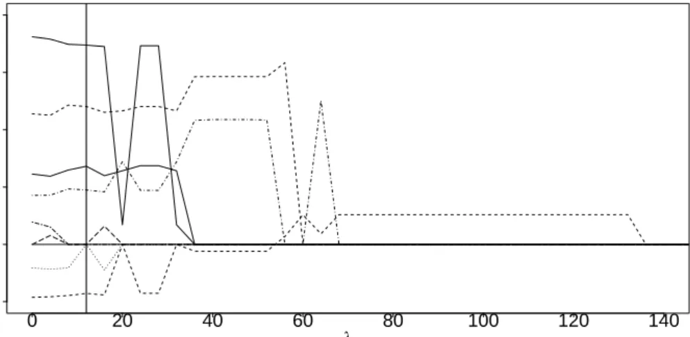
For selection of the penalty parameter λ for the glmmLasso 5-fold cross-validation was employed. The corresponding validation scores of prediction errors, based on the deviance, can be found in Figure 5. The cross-validation curve indicates that penalization clearly improves over ordinary fitting procedures that are obtained forλ= 0.

The results for the estimation of fixed effects, over-dispersion parameter ˆΦ and ˆσb for the

glmmPQLfunction and for theglmmLassoalgorithm are given in Table 6 and the correspond-ing coefficient built-ups are illustrated in Figure 6. TheglmmLasso algorithm suggests that “unfairness”, “ball possession” and “tackles” are not needed in the predictor, which are all three far away from significance concerning the standard errors of theglmmPQLfunction given in brackets.

glmmPQL glmmLasso intercept 3.860 (0.029) 3.858 (0.031) transfer spendings 0.179 (0.061) 0.174 (0.083) transfer spendings2 _{-0.046 (0.015) -0.043 (0.023)} unfairness -0.022 (0.028) -transfer receipts 0.043 (0.033) 0.047 (0.030) ball possession 0.008 (0.043) -tackles 0.015 (0.041) -attendance 0.059 (0.031) 0.068 (0.031) sold out 0.113 (0.033) 0.120 (0.031) ˆ σb 0.000 0.005 (0.012) ˆ Φ 1.637 1.394

Table 6: Estimates for the German Bundesliga data withglmmPQLfunction andglmmLassoalgorithm

(standard errors in brackets)

0 20 40 60 80 100 120 140 −0.05 0.05 0.10 0.15 0.20 λ β ^

Figure 6: Coefficient built-ups for theglmmLassofor the German Bundesliga data; the optimal value

of the penalty parameterλis shown by the vertical line

With variable selection the estimated dispersion parameter is not far away from one, so that the Poisson model seems adequate. TheglmmPQL function provides a very low standard deviation (ˆσb=0.000002) of the random intercepts, while theglmmLassomodel leads to results

that support the application of a random effects model, indicating that each soccer team has an individual bases level of points. In Figure 7 the quadratic effect of the variable “transfer spendings” is presented. Both approaches estimate very similar functions.

In addition we show the estimated random intercepts of the glmmLassofunctions for the 23 different soccer teams, that played in the German Bundesliga during the seasons 2007/2008 to 2009/2010. They can be seen as representing the team-specific playing ability that is not covered by the explanatory variables (see Table 7).

−1 0 1 2 3 4 −0.2 −0.1 0.0 0.1 0.2 transfer spendings f(tr ansf er spendings)

Figure 7: Estimated smooth effects computed with the glmmPQL model (dashed line) and the

glmmLassomodel (solid line) for the German Bundesliga data

For example the VfL Wolfsburg owns a small soccer stadium with a low number of ticket sold outs and was nevertheless rather successful in the last three years, so as a consequence its team-specific parameter is quite enhanced. The reverse effect could be observed e.g. for the FC Bayern M¨unchen. The club has earned by far the most points on average, but as it exhibits a rather high average attendance, with the stadium being permanently sold out, it got a relatively low random intercept, though being the most successful club in the league during the last three seasons.

4.2

CD4 Aids Study

The data were collected within the Multicenter AIDS Cohort Study (MACS). In the study about 5000 infected gay or bisexual men from Baltimore, Pittsburgh, Chicago and Los Angeles have been observed since 1984 (see Kaslow et al., 1987; Zeger and Diggle, 1994). The human immune deficiency virus (HIV) causes AIDS by attacking an immune cell called the CD4+ cell which coordinates the body’s immunoresponse to infectious viruses and hence reduces a person’s resistance against infection. According to Diggle et al. (2002) an uninfected individual has around 110 cells per milliliter of blood and since the number of CD4+ cells decreases with time from infection, one can use an infected person’s CD4+ cell number to check disease progression. Within the MACS, n = 369 seroconverters with a total of Pn_i=1Ti = 2376

measurements were included with the number of CD4+ cells being the interesting response variable. Covariates include the time since seroconversion ranging from 3 years before to 6 years after seroconversion, packs of cigarettes a day, recreational drug use (yes/no), number of sexual partners, age and a mental illness score (cesd). For observationtof individuali, the

Team ˆbi (glmmLasso) ˆbi (glmmPQL) VfL Wolfsburg 0.060 2.66_·10−4 VfB Stuttgart 0.056 2.76_·10−4 Bayer 04 Leverkusen 0.054 2.52_·10−4 Werder Bremen 0.049 2.23·10−4 FSV Mainz 05 0.022 7.70_·10−5 Hertha BSC 0.021 9.90_·10−5 Karlsruher SC 0.019 7.41·10−5 Borussia Dortmund 0.016 1.08_·10−4 FC Bayern M¨unchen 0.011 5.72·10−5 Hannover 96 0.008 3.83_·10−5 Energie Cottbus 0.007 1.79_·10−5 FC Schalke 04 -0.002 -8.64·10−6 Eintracht Frankfurt -0.006 -2.18_·10−5 Hansa Rostock -0.007 2.59·10−5 VfL Bochum -0.014 -7.22_·10−5 SC Freiburg -0.015 -5.93_·10−5 Arminia Bielefeld -0.018 -7.83·10−4 MSV Duisburg -0.020 7.31_·10−5 1899 Hoffenheim -0.032 -1.67_·10−4 Hamburger SV -0.037 -2.52_·10−4 1. FC N¨urnberg -0.051 -2.09_·10−4 FC K¨oln -0.059 -2.54·10−4 Borussia M’gladbach -0.062 2.69_·10−4

Table 7: Estimated random intercepts for German Bundesliga teams usingglmmLasso.

model that is considered has the form

g(µit) = β0+ timeitβ1+ time2itβ2+ time3itβ3+ time4itβ4+ drugsitβ5

+ partnersitβ6+ cigarettesitβ7+ cesditβ8+ ageitβ9+bi,

with bi ∼ N(0, σ2b). Again we fit an over-dispersed Poisson model with natural link while

the over-dispersion parameter Φ is estimated using (10). Our main objective is the typical time course of CD4+ decay and the variability across subjects. Earlier studies (e.g. Tutz and Reithinger, 2007, Groll and Tutz, 2011) have shown, that the time effect is nonlinear, so we additionally considered some higher powers of “time”.

The chosen penalty parameterλfor the glmmLassoagain was rather small,λopt= 21000,

and consequently almost all of the variables are included. The results for theglmmLasso al-gorithm and for theglmmPQL function are given in Table 8 and the corresponding coefficient

built-ups are illustrated in Figure 8. Both approaches yield very similar estimates. The incor-porated selection procedure suggests that drug use and age are not needed in the predictor.

0 10000 20000 30000 40000 50000 −0.20 −0.10 0.00 0.05 λ β ^

Figure 8: Coefficient built-ups for theglmmLassofor the CD4 data; the optimal value of the penalty

parameterλis shown by the vertical line

glmmPQL glmmLasso Intercept 6.643 (0.028) 6.665 (0.026) Time -0.199 (0.011) -0.200 (0.012) Time2 _{-0.014 (0.004) -0.014 (0.004)} Time3 _{0.014 (0.003) 0.014 (0.002)} Time4 _{-0.002 (0.000) -0.002 (0.000)} Drugs 0.029 (0.023) -Partners 0.004 (0.003) 0.004 (0.003) Packs of Cigarettes 0.042 (0.009) 0.049 (0.007) Mental illness score (cesd) -0.003 (0.010) -0.003 (0.001)

Age 0.000 (0.002)

-ˆ

σb 0.298 0.252 (0.091)

ˆ

Φ 63.439 76.943

Table 8: Estimates for the MACS withglmmPQLfunction andglmmLassoalgorithm (standard

devia-tions in brackets)

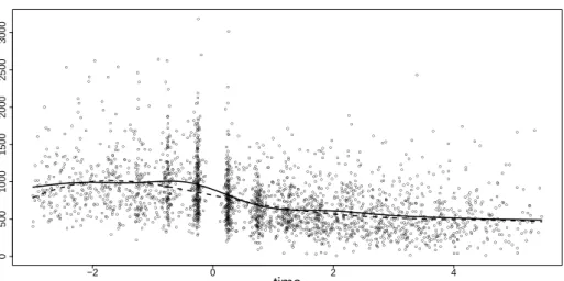
The smooth effect of time on CD4+ cell decay for our over-dispersed Poisson model together with the data is shown in Figure 9. Besides, we show the smooth effect obtained by a penalized basis function approach which is implemented in the gamm function of the R-package mgcv (Wood, 2006). All other variables have been kept constant at their means. Obviously the variable time has a negative effect on the CD4+ cell number.

● ● ● ● ● ● ● ● ● ● ● ● ● ● ● ● ● ● ● ● ● ● ● ● ● ● ● ● ● ● ● ● ● ● ● ● ● ● ● ● ● ● ● ● ● ● ● ● ● ● ● ● ● ● ● ● ● ● ● ● ● ● ● ● ● ● ● ● ● ● ● ● ● ● ● ● ● ● ● ● ● ● ● ● ● ● ● ● ● ● ● ● ● ● ● ● ● ● ● ● ● ● ● ● ● ● ● ● ● ● ● ● ● ● ● ● ● ● ● ● ● ● ● ● ● ● ● ● ● ● ● ● ● ● ● ● ● ● ● ● ● ● ● ● ● ● ● ● ● ● ● ● ● ● ● ● ● ● ● ● ● ● ● ● ● ● ● ● ● ● ● ● ● ● ● ● ● ● ● ● ● ● ● ● ● ● ● ● ● ● ● ● ● ● ● ● ● ● ● ● ● ● ● ● ● ● ● ● ● ● ● ● ● ● ● ● ● ● ● ● ● ● ● ● ● ● ● ● ● ● ● ● ● ● ● ● ● ● ● ● ● ● ● ● ● ● ● ● ● ● ● ● ● ● ● ● ● ● ● ● ● ● ● ● ● ● ● ● ● ● ● ● ● ● ● ● ● ● ● ● ● ● ● ● ● ● ● ● ● ● ● ● ● ● ● ● ● ● ● ● ● ● ● ● ● ● ● ● ● ● ● ● ● ● ● ● ● ● ● ● ● ● ● ● ● ● ● ● ● ● ● ● ● ● ● ● ● ● ● ● ● ● ● ● ● ● ● ● ● ● ● ● ● ● ● ● ● ● ● ● ● ● ● ● ● ● ● ● ● ● ● ● ● ● ● ● ● ● ● ● ● ● ● ● ● ● ● ● ● ● ● ● ● ● ● ● ● ● ● ● ● ● ● ● ● ● ● ● ● ● ● ● ● ● ● ● ● ● ● ● ● ● ● ● ● ● ● ● ● ● ● ● ● ● ● ● ● ● ● ● ● ● ● ● ● ● ● ● ● ● ● ● ● ● ● ● ● ● ● ● ● ● ● ● ● ● ● ● ● ● ● ● ● ● ● ● ● ● ● ● ● ● ● ● ● ● ● ● ● ● ● ● ● ● ● ● ● ● ● ● ● ● ● ● ● ● ● ● ● ● ● ● ● ● ● ● ● ● ● ● ● ● ● ● ● ● ● ● ● ● ● ● ● ● ● ● ● ● ● ● ● ● ● ● ● ● ● ● ● ● ● ● ● ● ● ● ● ● ● ● ● ● ● ● ● ● ● ● ● ● ● ● ● ● ● ● ● ● ● ● ● ● ● ● ● ● ● ● ● ● ● ● ● ● ● ● ● ● ● ● ● ● ● ● ● ● ● ● ● ● ● ● ● ● ● ● ● ● ● ● ● ● ● ● ● ● ● ● ● ● ● ● ● ● ●● ● ● ● ● ● ● ● ● ● ● ● ● ● ● ● ● ● ● ● ● ● ● ● ● ● ● ● ● ● ● ● ● ● ● ● ● ● ● ● ● ● ● ● ● ● ● ● ● ● ● ● ● ● ● ● ● ● ● ● ● ● ● ● ● ● ● ● ● ● ● ● ● ● ● ● ● ● ● ● ● ● ● ● ● ● ● ● ● ● ● ● ● ● ● ● ● ● ● ● ● ● ● ● ● ● ● ● ● ● ● ● ● ● ● ● ● ● ● ● ● ● ● ● ● ● ● ● ● ● ● ● ● ● ● ● ● ● ● ● ● ● ● ● ● ● ● ● ● ● ● ● ● ● ● ● ● ● ● ● ● ● ● ● ● ● ● ● ● ● ● ● ● ● ● ● ● ● ● ● ● ● ● ● ● ● ● ● ● ● ● ● ● ● ● ● ● ● ● ● ● ● ● ● ● ● ● ● ● ● ● ● ● ● ● ● ● ● ● ● ● ● ● ● ● ● ● ● ● ● ● ● ● ● ● ● ● ● ● ● ● ● ● ● ● ● ● ● ● ● ● ● ● ● ● ● ● ● ● ● ● ● ● ● ● ● ● ● ● ● ● ● ● ● ● ● ● ● ● ● ● ● ● ● ● ● ● ● ● ● ● ● ● ● ● ● ● ● ● ● ● ● ● ● ● ● ● ● ● ● ● ● ● ● ● ● ● ● ● ● ● ● ● ● ● ● ● ● ● ● ● ● ● ● ● ● ● ● ● ● ● ● ● ● ● ● ● ● ● ● ● ● ● ● ● ● ● ● ● ● ● ● ● ● ● ● ● ● ● ● ● ● ● ● ● ● ● ● ● ● ● ● ● ● ● ● ● ● ● ● ● ● ● ● ● ● ● ● ● ● ● ● ● ● ● ● ● ● ● ● ● ● ● ● ● ● ● ● ● ● ● ● ● ● ● ● ● ● ● ● ● ● ● ● ● ● ● ● ● ● ● ● ● ● ● ● ● ● ● ● ● ● ● ● ● ● ● ● ● ● ● ● ● ● ● ● ● ● ● ● ● ● ● ● ● ● ● ● ● ● ● ● ● ● ● ● ● ● ● ● ● ● ● ● ● ● ● ● ● ● ● ● ● ● ● ● ● ● ● ● ● ● ● ● ● ● ● ● ● ● ● ● ● ● ● ● ● ● ● ● ● ● ● ● ● ● ● ● ● ● ● ● ● ● ● ● ● ● ● ● ● ● ● ● ● ● ● ● ● ● ● ● ● ● ● ● ● ● ● ● ● ● ● ● ● ● ● ● ● ● ● ● ● ● ● ● ● ● ● ● ● ● ● ● ● ● ● ● ● ● ● ● ● ● ● ● ● ● ● ● ● ● ● ● ● ● ● ● ● ● ● ● ● ● ● ● ● ● ● ● ● ● ● ● ● ● ● ● ● ● ● ● ● ● ● ● ● ● ● ● ● ● ● ● ● ● ● ● ● ● ● ● ● ● ● ● ● ● ● ● ● ● ● ● ● ● ● ● ● ● ● ● ● ● ● ● ● ● ● ● ● ● ● ● ● ● ● ● ● ● ● ● ● ● ● ● ● ● ● ● ● ● ● ● ● ● ● ● ● ● ● ● ● ● ● ● ● ● ● ● ● ● ● ● ● ● ● ● ● ● ● ● ● ● ● ● ● ● ● ● ● ● ● ● ● ● ● ● ● ● ● ● ● ● ● ● ● ● ● ● ● ● ● ● ● ● ● ● ● ● ● ● ● ● ● ● ● ● ● ● ● ● ● ● ● ● ● ● ● ● ● ● ● ● ● ● ● ● ● ● ● ● ● ● ● ● ● ● ● ● ● ● ● ● ● ● ● ● ● ● ● ● ● ● ● ● ● ● ● ● ● ● ● ● ● ● ● ● ● ● ● ● ● ● ● ● ● ● ● ●● ● ● ● ● ● ● ● ● ● ● ● ● ● ● ● ● ● ● ● ● ● ● ● ● ● ● ● ● ● ● ● ● ● ● ● ● ● ● ● ● ● ● ● ● ● ● ● ● ● ● ● ● ● ● ● ● ● ● ● ● ● ● ● ● ● ● ● ● ● ● ● ● ● ● ● ● ● ● ● ● ● ● ● ● ● ● ● ● ● ● ● ● ● ● ● ● ● ● ● ● ● ● ● ● ● ● ● ● ● ● ● ● ● ● ● ● ● ● ● ● ● ● ● ● ● ● ● ● ● ● ● ● ● ● ● ● ● ● ● ● ● ● ● ● ● ● ● ● ● ● ● ● ● ● ● ● ● ● ● ● ● ● ● ● ● ● ● ● ● ● ● ● ● ● ● ● ● ● ● ● ● ● ● ● ● ● ● ● ● ● ● ● ● ● ● ● ● ● ● ● ● ● ● ● ● ● ● ● ● ● ● ● ● ● ● ● ● ● ● ● ● ● ● ● ● ● ● ● ● ● ● ● ● ● ● ● ● ● ● ● ● ● ● ● ● ● ● ● ● ● ● ● ● ● ● ● ● ● ● ● ● ● ● ● ● ● ● ● ● ● ● ● ● ● ● ● ● ● ● ● ● ● ● ● ● ● ● ● ● ● ● ● ● ● ● ● ● ● ● ● ● ● ● ● ● ● ● ● ● ● ● ● ● ● ● ● ● ● ● ● ● ● ● ● ● ● ● ● ● ● ● ● ● ● ● ● ● ● ● ● ● ● ● ● ● ● ● ● ● ● ● ● ● ● ● ● ● ● ● ● ● ● ● ● ● ● ● ● ● ● ● ● ● ● ● ● ● ● ● ● ● ● ● ● ● ● ● ● ● ● ● ● ● ● ● ● ● ● ● ● ● ● ● ● ● ● ● ● ● ● ● ● ● ● ● ● ● ● ● ● ● ● ● ● ● ● ● ● ● ● ● ● ● ● ● ● ● ● ● ● ● ● ● ● ● ● ● ● ● ● ● ● ● ● ● ● ● ● ● ● ● ● ● ● ● ● ● ● ● ● ● ● ● ● ● ● ● ● ● ● ● ● ● ● ● ● ● ● ● ● ● ● ● ● ● ● ● ● ● ● ● ● ● ● ● ● ● ● ● ● ● ● ● ● ● ● ● ● ● ● ● ● ● ● ● ● ● ● ● ● ● ● ● ● ● ● ● ● ● ● ● ● ● ● ● ● ● ● ● ● ● ● ● ● ● ● ● ● ● ● ● ● ● ● ● ● ● ● ● ● ● ● ● ● ● ● ● ● ● ● ● ● ● ● ● ● ● ● ● ● ● ● ● ● ● ● ● ● ● ● ● ● ● ● ● ● ● ● ● ● ● ● ● ● ● ● ● ● ● ● ● ● ● ● ● ● ● ● ● ● ● ● ● ● ● ● ● ● ● ● ● ● ● ● ● ● ● ● ● ● ● ● ● ● ● ● ● ● ● ● ● ● ● ● ● ● ● ● ● ● ● ● ● ● ● ● ● ● ● ● ● ● ● ● ● ● ● ● ● ● ● ● ● ● ● ● ● ● ● ● ● ● ● ● ● ● ● ● ● ● ● ● ● ● ● ● ● ● ● ● ● ● ● ● ● ● ● ● ● ● ● ● ● ● ● ● ● ● ● ● ● ● ● ● ● ● ● ● ● ● ● ● ● ● ● ● ● ● ● ● ● ● ● ● ● ● ● ● ● ● ● ● ● ● ● ● ● ● ● ● ● ● ● ● ● ● ● ● ● ● ● ● ● ● ● ● ● ● ● ● ● ● ● ● ● ● ● ● ● ● ● ● ● ● ● ● ● ● ● ● ● ● ● ● ● ● ● ● ● ● ● ● ● ● ● ● ● ● ● ● ● ● ● ● ● ● ● ● ● ● ● ● ● ● ● ● ● ● ● ● ● ● ● ● ● ● ● ● ● ● ● ● ● ● ● ● ● ● ● ● −2 0 2 4 0 500 1000 1500 2000 2500 3000 time cd4

Figure 9: Smoothed time effect (CD4+ number of cellsversustime) from MACS forgamm(solid line)

andglmmLasso(dashed line).

4.3

Forest health Data

The forest health data has been considered in previous studies, for example in Kneib et al. (2009) and Tutz and Groll (2011). In this application, the health status of beeches at 83 observation plots located in a northern Bavarian forest district has been assessed in visual forest health inventories carried out between 1983 and 2004. Originally, the health status is classified on an ordinal scale, where the nine possible categories denote different degrees of defoliation. Figure 10 shows a histogram of the nine defoliation classes indicating that no trees were observed in the last two categories. We are now only interested in wether a tree is healthy or not, so we model the dichotomized response variable defoliation with categories 1 (not healthy; defoliation above or equal 12.5%) and 0 (healthy; no defoliation; 0.0%). In Kneib et al. (2009) a brief description of the covariates in the data set is presented, which is found in Table 9.

Covariate Description

age age of the tree in years (continuous, 7≤age≤234)

elevation elevation above sea level in meters (continuous, 250≤elevation≤480) inclination inclination of slope in percent (continuous, 0≤inclination≤46) soil depth of soil layer in centimeters (continuous, 9≤soil≤51) canopy density of forest canopy in percent (continuous, 0≤canopy≤1) stand type of stand (categorical, 1 = deciduous forest, -1 = mixed forest) fertilisation fertilisation (categorical, 1 = yes, -1 = no)

humus thickness of humus layer in 5 categories (ordinal, higher categories represent higher proportions)

moisture level of soil moisture (categorical, 1 = moderately dry, 2 = moderately moist, 3 = moist or temporary wet)

saturation base saturation (ordinal, higher categories indicate higher base saturation)

0% 12.5% 25% 37.5% 50% 62.5% 75% 87.5% 100% 0.0 0.2 0.4 0.6 0.8 1.0

Figure 10: Relative frequencies of the nine defoliation classes for all observation plots and all time points for the forest health data

As Kneib et al. (2009) identified a nonlinear effect of “age”, we again include some higher powers of “age” into our model, which results in the following predictor:

g(πit) = β0+ ageitβ1+ age2itβ2+ age3itβ3+ age4itβ4+ elevationitβ5

+ inclinationitβ6+ soilitβ7+ canopyitβ8+ fertilisationitβ9+ standitβ10

+ humus0itβ11+ humus2itβ12+ humus3itβ13+ humus4itβ14+ saturation1itβ15

+ saturation3itβ16+ saturation4itβ17+ moisture1itβ18+ moisture3itβ19+bi,

whereπit=µit denotes the expected probability of defoliation for observation areaiat timet

andbi∼N(0, σb2) again represent cluster-specific random intercepts. We fit a binomial model

with logit-link, building groups for the categorial variables “humus”, “moisture” and “satura-tion”. For this purpose we use the extended algorithm for categorical predictors from Section 3.3. The results for the parameter estimates can be found in Table 10 and the corresponding coefficient built-ups are illustrated in Figure 11.

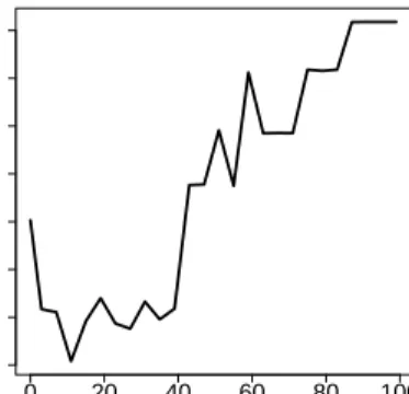
The penalty parameterλfor theglmmLassoagain was determined by 5-fold cross-validation on the interval [0; 300]. The chosen parameter was rather small, λopt = 10, indicating that

penalization only slightly improves the fit compared to ordinary fitting procedures which are obtained for λ = 0 and consequently almost all of the variables are included. The smooth effect of age on tree defoliation for our binomial model with logit-link is shown in Figure 12, again compared to the smooth effect obtained by the penalized basis function approach using the gamm function. Obviously with increasing age of the trees the probability of defoliation increases in a non-linear fashion.

0 50 100 150 −4 −3 −2 −1 0 1 λ β ^

Figure 11: Coefficient built-ups for the glmmLassofor the forest health data; the optimal value of

the penalty parameterλis shown by the vertical line

glmmPQL glmmLasso Intercept -7.226 (2.719) -5.353 (1.923) age 0.401 (0.080) 0.391 (0.078) age2 _{-0.007 (0.001) -0.006 (0.001)} age3 _{0.000 (0.000) 0.000 (0.000)} age4 _{0.000 (0.000) 0.000 (0.000)} elevation 0.006 (0.005) -inclination 0.005 (0.025) -soil -0.043 (0.024) -0.039 (0.026) canopy -3.550 (0.539) -3.554 (0.568) fertilisation -1.422 (0.828) -1.130 (0.773) stand 0.934 (0.464) 0.889 (0.456) humus0 -0.486 (0.155) -0.472 (0.180) humus2 0.316 (0.131) 0.323 (0.147) humus3 0.313 (0.155) 0.306 (0.169) humus4 0.036 (0.218) 0.011 (0.238) saturation1 0.471 (0.533) 0.658 (0.483) saturation3 -0.254 (0.557) -0.422 (0.524) saturation4 0.102 (0.699) 0.023 (0.652) moisture1 -0.916 (0.522) -0.968 (0.498) moisture3 1.112 (0.379) 1.011 (0.365) ˆ σb 1.816 1.845 (0.177)

Table 10: Estimates for the forest health data

4.4

Jimma Infant Survival Study

The Jimma Infant Survival Differential Longitudinal Study is a cohort study investigating the live births which took place in the town of Jimma in Ethiopia during a one year period from September 1992 until September 1993. An extensive description can be found in Lesaffre et al. (1999). The study covers 8000 households with live births in the said period. Following Lesaffre

0 50 100 150 200 −6 −4 −2 0 2 4 age f(age)

Figure 12: Smoothed age effect for the forest health data with gamm (solid line) and glmmLasso

(dashed line).

et al. (1999) and Tutz and Reithinger (2007), 495 singleton live births have been considered and monitored for a one year period in order to determine the risk factors for infant mortality. A good indicator of a child’s health status is the body weight. Hence, to determine possible influence factors on growth of the children, we use the (logarithmic) body weight (in kg) as response variable together with some socio-economic and demographic as well as some prenatal and delivery-related covariates. A brief description of all considered covariates can be found in Table 11.

Covariate Description

age age of the child in days (continuous, 0≤age≤385) ageM age of the mother in years (continuous, 14≤ageM≤50)

education educational level of the mother (categorical, 1 = illiterate, 2 = read and write, 3 = elementary school, 4 = junior high school, 5 = high school, 6 = college and above) delivery place of delivery (categorical, 1 = hospital, 2 = health center, 3 = home)

visits number of antenatal visits (categorical, 0,≥1)

month month of birth (categorical, 1 = Jan. - June, 0 = July - Dec.) sex sex of the child (categorical, 1 = male, 0 = female)

marital marital status of mother (categorical, 1 = married, 2 = divorced, 3 = widowed, 4 = never married)

status occupational status of mother (categorical, 1 = unemployed, 0 = employed)

Table 11: Description of covariates for the Jimma data

Tutz and Reithinger (2007) identified a nonlinear effect of “age”, therefore we include also “age2_{” into our model, resulting in the following predictor:}

g(µit) = β0+ ageitβ1+ age2itβ2+ ageMitβ3+ education1itβ4+ education2itβ5

+ education3itβ6+ education4itβ7+ education5itβ8+ delivery1itβ9

+ delivery2itβ10+ visitsitβ11+ monthitβ12+ sexitβ13+ marital1itβ14

+ marital2itβ15+ marital3itβ16+ statusitβ17+b0i+ ageitb1i+ age2itb2i,

where µit denotes the expected body weight of child i at time t and bi = (b0i, b1i, b2i)T ∼

N(000,Q) represent child-specific random intercepts and random slopes on age and squared age. The continuous variables age, squared age and age of the mother have been standardized. We fit a normal distribution model with log-link, building groups for the categorial variables “ed-ucation”, “delivery” and “marital”. So again the extended algorithm for categorical predictors from Section 3.3 is required. The estimates for the standard deviations of the random effects for the standardized model are presented in Table 12.

glmmPQL glmmLasso ˆ σb0 0.121 0.153 (0.046) ˆ σb1 0.037 0.000 (0.051) ˆ σb2 0.000 0.069 (0.045)

Table 12: Estimates for the standard deviations of the random effects for the Jimma data with

glmmPQLfunction andglmmLassoalgorithm (standard deviations in brackets)

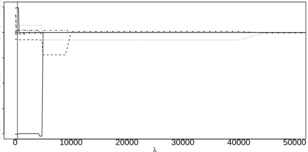
The results for the estimated linear effects corresponding to the original scaling of the variables can be found in Table 13 and the corresponding coefficient built-ups are illustrated in Figure 14. The cross-validation score is plotted against the penalty parameterλin Figure 13. Again penalization improves ordinary fitting procedures obtained forλ= 0 and a rather sparse model is chosen with a clearly non-linear influence of the child’s age and a linear influence of the variables “delivery”, “visits” and “sex”.

Keeping all other variables constant at their means, the child-specific smooth effects of the children’s age on the body weight is shown in Figure 15 and compared to the child-specific smooth effects obtained by the unregularized approach using theglmmPQLfunction, see Figure 16. It seems that there is somewhat more variation between theglmmLassocurves which may be due to the bigger variance estimate of the random intercept. As was to be expected, with increasing age of the children their body weight increases, at first relatively fast, but slowing down after the first 150 days. The main feature of the penalized approach is that variables that also turn out to be non-influential are automatically selected.

λ

CV score

0 1000 2000 3000

1125.4

1125.6

Figure 13: 5-fold cross-validation scores for theglmmLassoas function of penalty parameter λfor

the Jimma data

0 500 1000 1500 2000 2500 3000 −0.10 0.00 0.05 0.10 0.15 λ β ^

Figure 14: Coefficient built-ups for the glmmLassofor the Jimma data; the optimal value of the

penalty parameterλis shown by the vertical line

5

Concluding Remarks

Several procedures for variable selection based onL1-penalties have been proposed. The

pro-cedures yield stable estimates in cases where methods that do not include variable selection typically fail because of the complexity of the fitting task. The method allows to include cat-egorical predictors that are selected predictor or omitted as a whole predictor in the spirit of the group lasso. It is straightforward to extend the approach to include more complex penalty terms, for example, the elastic net penalty or hierarchical penalty terms as proposed by Zhao et al. (2009).

glmmPQL glmmLasso Intercept 1.213 (0.052) 1.257 (0.045) age 0.005 (0.000) 0.005 (0.000) age2 _{-0.000 (0.000) -0.000 (0.000)} ageM 0.002 (0.001) -education1 -0.077 (0.041) -education2 -0.078 (0.042) -education3 -0.032 (0.041) -education4 -0.017 (0.041) -education5 -0.018 (0.040) -delivery1 0.021 (0.019) 0.028 (0.019) delivery2 -0.024 (0.017) -0.026 (0.016) visits -0.045 (0.013) -0.053 (0.010) month -0.024 (0.012) -sex 0.081 (0.012) 0.080 (0.013) marital1 0.057 (0.025) -marital2 0.104 (0.057) -marital3 0.056 (0.038) -occupational 0.001 (0.016)

-Table 13: Estimated linear effects for the Jimma data withglmmPQLfunction andglmmLassoalgorithm (standard deviations in brackets)