An Alternative to the Youla Parameterization for H
∞
Controller Design
Hamid Khatibi and Alireza Karimi
Abstract— AllH∞controllers of a SISO LTI system are param-eterized thanks to the relation between the Bounded Real Lemma and the Positive Real Lemma. This new parameterization shares the features of Youla parameterization, namely the convexity
of H∞ norm constraints for the closed-loop transfer functions.
However, by contrast to Youla parameterization, it can deal with any controller order and any controller structure, e.g. PID controllers. Moreover, it can be easily used for systems with polytopic uncertainty. For polytopic systems, the proposed parameterization provides a convex inner approximation of the
set of all H∞ controllers, which can be enlarged by increasing
the controller order. The effectiveness of the proposed method is shown via simulation results.
I. INTRODUCTION
The Youla parameterization [1] is probably the most well-known controller parameterization, which parameterizes all stabilizing controllers of a system, over an infinite dimensional space. The main advantage of this parameterization is that all closed-loop sensitivity functions are affine w.r.t. the so-called
Q parameter and hence it can be employed forH∞ controller
design in a convex optimization problem. The Youla param-eterization has two major disadvantages. First, it cannot deal with fixed-order controllers or enforce a prescribed controller structure such as PID. Second, it depends on system parameters and therefore it cannot be used for systems with parametric uncertainty such as polytopic systems.
Polytopic uncertainty is one of the most general ways of capturing physical parameter uncertainty, multi-model systems and the well-known interval systems, and has attracted many robust controller designers recently. In [2] a convex param-eterization of fixed-order controllers for polytopic systems is given based on the polynomial positivity. It gives a stabilizing controller (a feasible point), which closely depends on a so-called central polynomial. This method is used for convex
parameterization ofH∞controllers in [3], however, again the
solution depends on the choice of the central polynomial. The effect of this choice on the convex set of stabilizing fixed-order controllers is studied in [4]. In a similar approach, it is shown that the dependence on the central polynomial can be relaxed by increasing the controller order [5]. This parameterization covers all stabilizing controllers in an infinite dimensional space, whose inner approximation for fixed-order controllers coincides with the results of [2] and [4]. The advantage of this parameterization w.r.t. Youla parameterization is that it parameterizes all stabilizing controllers of a polytopic system and, in addition, it can deal with any controller structure and a prescribed order. However, in contrary to Youla parameteri-zation, it does not lead to affine closed-loop transfer functions w.r.t. the controller parameters.
An alternative to Youla parameterization of all H∞
con-trollers is given in this paper. The main advantage of this new
parameterization is that it can enforce any controller structure and order. Moreover, similar to Youla parameterization and in contrary to the parameterization of [5], all closed-loop transfer functions become affine w.r.t. the variables, which enables a
convex parameterization of allH∞controllers. Furthermore, it
can be easily employed for polytopic systems to give a
con-vex inner approximation of all H∞ controllers. The problem
considered in this paper is very similar to that of [3], where a
convex parameterization of fixed-orderH∞controllers is given
using the properties of positive polynomials. However, in this paper a different approach based on the strict positive realness of two transfer functions with the same Lyapunov matrix in the inequality of the Kalman-Yakubovic-Popov lemma is em-ployed. Moreover, it is shown that by increasing the controller order the dependence on the central polynomial can be relaxed. In addition, for continuous-time systems it is shown that it is
possible to minimize the desired H∞ norm, whereas in [3],
the iterative bisection algorithm should be used to find the
minimum value of the desiredH∞ norm.
The rest of the paper is organized as follows. Some notations and preliminaries are briefly recalled in Section II. Main results are presented in Section III, where the new convex constraints
that satisfyH∞performance specifications are introduced. The
simulation results in Section IV illustrate the effectiveness of the proposed synthesis method and concluding remarks are given in Section V. Finally, it is shown in Appendix that for continuous-time systems, it is possible to minimize the desired
H∞ norm in a convex optimization problem instead of using
the iterative bisection algorithm.
II. PRELIMINARIES
The goal is to give a convex parameterization of all H∞
controllers for a known system and then to extend the method for systems with polytopic uncertainty.
Consider a SISO LTI plant represented by a finite order rational transfer function G in discrete- or in continuous-time. Assume that N and M are the coprime factors of G such that
G=NM−1, N,M∈RH∞ (1)
where RH∞ is the set of proper stable rational transfer
functions with bounded infinity norm. It is shown in [5] that the set of all stabilizing controllers of (1) is given by :
Ks:{K=XY−1|MY+NX∈S} (2)
where X,Y ∈RH∞ and S is the convex set of all Strictly
Positive Real (SPR) transfer functions. Using the following lemma, this parameterization can be represented as LMIs :
Lemma 1: (the KYP lemma for discrete-time systems [6])
(ESPR in [7]) if and only if there exists a matrix P=PT >0 such that : ATPA−P ATPB−CT BTPA−C BTPB−D−DT <0 (3)
It is evident that A and B (with a controllable canonical
realization) are only related to the denominator of H(z)and are
therefore fixed in case H=MY+NX . The plant parameters
and the controller parameters (the optimization variables) ap-pear linearly in C and D. Hence, the above inequality becomes
an LMI because the variables P,C and D appear affinely in it.
The advantage of this parameterization is that it can be easily applied to polytopic and multi-model systems because, by contrast to the Youla parameterization, the controller pa-rameterization does not depend on the system parameters.
Consider a polytopic system with q vertices such that the i-th vertex consists of i-the parameters of i-the model Gi=NiMi−1,
where Ni and Mi∈RH∞ are the coprime factors of Gi. The
set of all models in this polytopic system can be represented by: G :{G=NM−1|N= q
∑
i=1 λiNi,M= q∑
i=1 λiMi} (4)whereλi≥0 and
q
∑
i=1
λi=1. The set of all stabilizing controllers for this polytopic system is given by [5] :
Kp:{K=XY−1|MiY+NiX∈S, i=1, . . . ,q} (5)
where X,Y ∈RH∞. The main drawback of this approach
is that the norm constraints on sensitivity functions are not convex with respect to X and Y, for example in the following sensitivity function:
S= (1+KG)−1= MY
MY+NX
. A solution to this problem is proposed in [5] by putting the constraints on numerator and denominator of S separately. This leads to the following optimization problem for a polytopic system : Minimize max i γi Subject to: MiY+NiX∈S for i=1, . . . ,q kMiY+NiX−1k∞<γi for i=1, . . . ,q kW1MiYk<1−γi for i=1, . . . ,q (6)
where the second and the third constraints together present
convexified approximation of the H∞ constraints kW1Sik<
1 for i=1, . . . ,q.
However, this approach is not able to minimize the H∞
performance index kW1Sik∞, i.e. we can just ensure that
kW1Sik∞<1,i=1, . . . ,q. Furthermore, since the desired H∞
norm is not related to the cost function, minimizing this cost
function generally leads to a higher kW1Sik∞. To overcome
these drawbacks, a new convex representation of the desired
H∞ norm is proposed in the next section.
III. MAINRESULT
To ensure the robust performance, we want to parameterize
all stabilizing controllers that satisfy some H∞ norm bounds
on some weighted transfer functions of the closed-loop sys-tem. However, for the simplicity reasons, we demonstrate the
method withH∞norm bound on only one sensitivity function.
Thus, without loss of generality, suppose that it is desired to have : kW1Sk∞= W1MY MY+NX ∞ <γ (7)
for a givenγ. It is well known that an infinity norm constraint
could be presented as LMIs via Bounded Real Lemma, if the denominator of its argument is fixed [8]. However, in this case, the controller parameters appear both in numerator
and denominator of W1S, which results in a Bilinear Matrix
Inequality (BMI) problem. In order to convexify this per-formance constraint, the relation between the Bounded Real Lemma and the Positive Real Lemma is employed. It is well known that (7) is equivalent to the SPRness of [9] :
(MY+NX)−γ−1W 1MY
(MY+NX) +γ−1W 1MY
(8) Therefore, the set of all controllers that result in a closed-loop system withkW1Sk∞<γfor a system G defined in (1), is given
by : K∞:{K=XY−1| (MY+NX)−γ−1W 1MY (MY+NX) +γ−1W 1MY ∈S} (9)
where X,Y ∈RH∞. Using the KYP lemma (Lemma 1 for
discrete-time systems), the SPRness of a transfer function with fixed denominator can be represented via LMIs. However, in (9), both numerator and denominator contain optimization variables and hence, the set is not convex in this form.
In the sequel, (9) is represented via LMIs. Moreover, it is shown that the resulting LMIs give the complete set of all
stabilizingH∞ controllers.
A. LMI representation
The following definitions and lemmas are required to pro-ceed.
Definition 1: A matrix A is called the state space matrix of
a monic polynomial p, if A is the controllable canonical state
space matrix of the transfer function 1/p.
Definition 2: Consider two equal-order monic polynomials
p1 and p2 and their state space matrices A1 and A2,
respec-tively. Then, p1 and p2(also A1 and A2) are called Common
Lyapunov stable, or CL-stable, if A1and A2satisfy a Lyapunov
inequality with the same Lyapunov matrix P, namely for
discrete-time systems∃P=PT>0 such that :
AT1PA1−P<0 and AT2PA2−P<0
Lemma 2: [7] A transfer function H is SPR if and only if
its numerator and denominator are CL-stable.
Definition 3: Two equal-order SPR transfer functions H1
(A1,B1,C1,D1) and (A2,B2,C2,D2)are called Common
Lya-punov Strictly Positive Real, or CL-SPR, if both satisfy the inequality of the KYP lemma (Inequality (3) for discrete-time systems) with the same Lyapunov matrix P.
Remark : A very simple consequence of the above definition
is that an SPR transfer function H1is CL-SPR with all positive
fixed transfer functions such as H2=1.
Lemma 3: An SPR transfer function H and its inverse H−1
are CL-SPR.
Proof: Using Schur complement on (3) for both H and
its inverse, the proof is obtained easily. Furthermore, the proof is similar for continuous-time systems.
Since the inequality of the KYP lemma contains the Lyapunov stability constraint in its first block, Lemma 3 covers Lemma 2.
The following corollary shows how a CL-SPR constraint results in a CL-stability constraint :
Corollary 1: If two transfer functions H1 and H2 are
CL-SPR then all of their numerator and denominator polynomials are CL-stable.
Proof: Suppose that there exists P=PT >0 satisfying
the inequality of the KYP lemma for both transfer functions
H1 and H2. Since the first block of this LMI is the same
as the Lyapunov stability criterion, the denominators of these two transfer functions are CL-stable. Furthermore, according to Lemma 3, the same matrix P satisfies the LMI of the KYP lemma for H1−1and H2−1, which means that the same P satisfies
Lyapunov stability criterion for the numerators of H1and H2.
Hence, all of the four polynomials are CL-stable with the same matrix P.
Remark : Any P=PT>0 that reveals the CL-stability of two polynomials, does not necessarily satisfy the LMI of the KYP lemma for their SPR ratio. Hence, the above lemma could be proved just in the mentioned direction.
According to Lemma 2, we need to have CL-stability between numerator and denominator polynomials of (9) to prove its SPRness. However, the SPRness constraint of (9) becomes a non-convex inequality due to the existence of variables in its denominator, which causes multiplication of variables in the first block of the inequality of the KYP lemma. Taking into account Corollary 1, it is possible to impose a CL-SPR constraint on the transfer functions of numerator and denominator of (9) instead of a CL-stability constraint on its numerator and denominator polynomials. This CL-SPR constraint brings conservatism if the denominators of the mentioned transfer functions are fixed. However, this conservatism can be removed by letting the order of the controller be increased, which is the same idea used in [5] in order to remove the conservatism of (2). The following theorem states the main result of this paper for a single system.
Theorem 1: Consider the numerator and the denominator
transfer functions of (9) :
(MY+NX)−γ−1W
1MY (10)
(MY+NX) +γ−1W1MY (11)
Then, the set of all stabilizing controllers that result in a
closed-loop system withkW1Sk∞<γ for a system G defined in (1),
is given by :
K∞:{K=XY−1| (10) and (11) be CL-SPR} (12)
where X,Y ∈RH∞.
Proof: Sufficiency: It should be shown that any controller
satisfying (12), satisfies the norm constraint (7) and stabilizes the closed-loop system too. Taking into account Corollary 1, the numerators of (10) and (11) are CL-stable because the
controller K=XY−1 satisfies the CL-SPR constraint on (10)
and (11). Thus, based on Lemma 2, this controller belongs to
the set represented in (9), which means that it satisfies theH∞
constraint in (7). Furthermore, since the SPRness is a convex constraint, having two SPR transfer functions (10) and (11),
results in the SPRness of their sum, which means that MY+
NX is SPR. Therefore, K belongs to the set of all stabilizing
controllersKs in (2).
Necessity: It should be shown that if K0=X0Y0−1 is a
stabilizing controller that satisfies (7), then it belongs to K∞
in (12). Suppose that X0,Y0∈RH∞are coprime factors of K0.
Then, (MY0+NX0)−γ−1W1MY0 (MY0+NX0) +γ−1W1MY0 (13) is SPR, but (MY0+NX0) +γ−1W1MY0 and (MY0+NX0)− γ−1W
1MY0are not CL-SPR. We should show that there exists
always a transfer function F such that (10) and (11) become
CL-SPR with X = X0F and Y =Y0F, which means that
K0= (X0F)(Y0F)−1 belongs to K∞ in (12). By taking F=
(MY0+NX0) +γ−1W1MY0, (10) and (11) respectively become
equal to the SPR transfer functions (13) and 1, which are
CL-SPR according to the remark after Definition 3. Hence, K0
belongs toK∞ in (12) with X=X0F and Y=Y0F.
To design a fixed-order controller, a fixed polynomial should be chosen for the denominators of (10) and (11). It is clear that by fixing these denominators, the convex feasibility set of the CL-SPR constraint of (12) would be an inner approximation
of the non-convex set of allH∞ stabilizing controllers of the
desired order. An unsuitable choice of this polynomial may cause a null feasibility set. This conservatism can be removed by letting the order of X and Y be increased. By increasing the
order of X and Y , not only someH∞stabilizing controllers of
the new orders are included in the feasible set of the problem, but also more controllers of lower orders enter in the feasible set as can be seen by the above proof. To develop a simulation program, X and Y can be approximated using different types of orthonormal basis functions. For instance, consider that X and Y are linearly parameterized by :
X= m
∑
i=0 xiβi ; Y= m∑
i=0 yiβi (14)whereβi=1/(z−ζ)i,i=0, . . . ,m are the basis functions. As
a result, the CL-SPR constraint in (12) becomes linear in the parameters of X and Y and can be represented by LMIs thanks
to the KYP lemma : K∞:{K=XY−1| P=PT >0, (15) ATPA−P ATPB−CT 1 BTPA−C 1 BTPB−D1−DT1 <0 , (16) ATPA−P ATPB−C2T BTPA−C2 BTPB−D2−DT2 <0} (17) where (A,B,C1,D1) and (A,B,C2,D2) are the controllable
canonical state space realizations of (10) and (11), respectively. The state matrix A is assumed to be identical for both real-izations because the denominators of both transfer functions are the same. Besides, B is always the same for controllable canonical realizations.
Using the above parameterization, any controller structure and order can be enforced, whereas in Youla parameterization it is not possible. Moreover, another important feature of this parameterization is that it can be easily applied to systems with polytopic uncertainty. The following theorem extends this method for polytopic systems.
Theorem 2: Consider the transfer functions of numerator
and denominator of (9) for each vertices of the system polytope defined in (4) :
(MiY+NiX)−γ−1W1MiY (18) (MiY+NiX) +γ−1W1MiY (19)
Then, any controller belonging to the convex set :
Kp∞:{K=XY−1|(18) and (19) be CL-SPR,i=1, . . . ,q} (20)
where X,Y∈RH∞, stabilizes the polytopic system and results
in a closed-loop polytopic system with kW1Sk∞<γ for all of
its members.
Proof: It should be shown that if (MiY +NiX)−
γ−1W
1MiY and (MiY+NiX)−γ−1W1MiY are CL-SPR for i=1, . . . ,q, then the controller K=XY−1stabilizes the whole system polytope and in addition, satisfieskW1Sk∞<γ for all
members of the polytopic system G defined in (4). For each
vertices of G, the sum of two SPR transfer functions (18)
and (19) results in the SPRness of MiY+NiX, i=1, . . . ,q. In
Theorem 2 of [5], it is proved that such a controller stabilizes
all members ofG. Next, we should prove robust performance
with this controller, i.e. that it satisfies theH∞norm constraint
for all members ofG. This is shown more easily via the LMI
representation of (20) : Kp ∞:{K=XY−1| Pi=PiT >0, i=1, . . . ,q ATP iA−Pi ATPiB−CTi1 BTPiA−Ci1 BTPiB−Di1−DTi1 <0 (21) ATP iA−Pi ATPiB−CTi2 BTPiA−Ci2 B TP iB−Di2−D T i2 <0} (22) where (A,B,Ci1,Di1) and (A,B,Ci2,Di2) are the controllable
canonical state space realizations of (18) and (19) respectively.
A is assumed to be identical for all transfer functions (18) and
(19), because of their identical denominators and B is fixed because of the realization. Since all these constraints, i.e. (21) and (22), are linear w.r.t. the parameters of the system vertices,
0.05 0.1 0.15 0.2 0.25 0.3 0.35 0.4 0.45 −5 0 5 10 15 20 Magnitude (dB) Frequency (Hz)
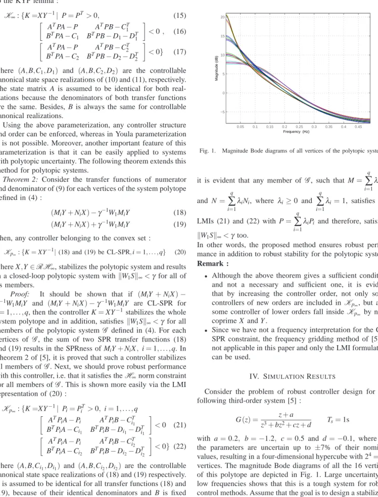
Fig. 1. Magnitude Bode diagrams of all vertices of the polytopic system.
it is evident that any member of G, such that M=
q
∑
i=1 λiMi and N= q∑
i=1λiNi, where λi ≥0 and
q
∑
i=1
λi =1, satisfies the
LMIs (21) and (22) with P=
q
∑
i=1
λiPi and therefore, satisfies kW1Sk∞<γ too.
In other words, the proposed method ensures robust perfor-mance in addition to robust stability for the polytopic system.
Remark :
• Although the above theorem gives a sufficient condition
and not a necessary and sufficient one, it is evident that by increasing the controller order, not only some
controllers of new orders are included in Kp
∞, but also
some controller of lower orders fall inside Kp
∞ by
non-coprime X and Y .
• Since we have not a frequency interpretation for the
CL-SPR constraint, the frequency gridding method of [5] is not applicable in this paper and only the LMI formulation can be used.
IV. SIMULATIONRESULTS
Consider the problem of robust controller design for the following third-order system [5] :
G(z) = z+a
z3+bz2+cz+d Ts=1s
with a=0.2, b=−1.2, c=0.5 and d=−0.1, where all
the parameters are uncertain up to ±7% of their nominal
values, resulting in a four-dimensional hypercube with 24=16
vertices. The magnitude Bode diagrams of all the 16 vertices of this polytope are depicted in Fig. 1. Large uncertainty in low frequencies shows that this is a tough system for robust control methods. Assume that the goal is to design a stabilizing
controller that contains an integrator, and kW1Sk∞ should be
1 2 3 4 5 6 7 8 9 0.55 0.6 0.65 0.7 0.75 0.8 0.85 0.9 0.95 1 1.05 γopt Controller order
Fig. 2. γopt for the system 26 versus the order of the controller for different
basis functions. Looking to the starting point from the highest curve, the basis function are chosen to haveζ=0,0.1,0.2,0.3,0.4,0.5 respectively.
weighting function W1(z)is chosen to be the same as in [5] :
W1(z) =
0.4902(z2−1.0431z+0.3263)
z2−1.282z+0.282 (23)
which is a low-pass weighting filter based on the inverse of the desired sensitivity function. The same coprime factorization of [5] is used for the nominal plant model:
N = z+0.2
(z−0.1)(z2−1.0431z+0.3263) (24)
M = z
3−1.2z2+0.5z−0.1
(z−0.1)(z2−1.0432z+0.3263) (25)
Note that the denominator of all coprime factors are identical
for all models in the polytopic system andζ=0.1 as in [5].
Before dealing with the polytopic system, we want to show the main advantage of the proposed method. That is, for a system without uncertainty, the proposed method can
achieve the optimal H∞ norm by increasing the controller
order, irrelevant to the choice of the basis functions. Using the MATLAB command hinfsyn for one of the system vertices
G1=
z−.186
z3−1.116z2+0.465z−0.093 (26)
a fifth-order controller withkW1Sk∞=0.552 is obtained. Fig.
2 shows that by increasing the controller order, the proposed
method converges to the optimum norm bound of kW1Sk∞,
independent of the choice of zeta in the basis functions. Next, we design a controller for the polytopic system. The problem in [5] does not become feasible for controller orders less than 5, because the second and the third line of (6) are sufficient conditions for kW1Sik∞<1. However,
using the proposed method in this paper, it becomes feasible
with a second-order controller. The controller K =XY−1 is
parameterized as follows : X=x1z 2+x 2z+x3 (z−0.1)2 , Y= (z−1)(y1z+y2) (z−0.1)2 0.05 0.1 0.15 0.2 0.25 0.3 0.35 0.4 0.45 −16 −14 −12 −10 −8 −6 −4 −2 Magnitude (dB) Frequency (Hz)
Fig. 3. Bode magnitude diagram of W1Si of all vertices of the polytopic
system with the second-order controller (27) (Solid) andγopt(Dotted).
0.05 0.1 0.15 0.2 0.25 0.3 0.35 0.4 0.45 −16 −14 −12 −10 −8 −6 −4 −2 0 2 4 6 Magnitude (dB) Frequency (Hz)
Fig. 4. Output sensitivity function of all vertices of the polytopic system with the second-order controller (27) (Solid), Bode magnitude diagram ofγopt/W1
(Dotted).
To solve the problem in MATLAB, YALMIP [10] is used as the interface and SDPT3 [11] as the solver. Using the iterative bisection algorithm, the optimal value ofγopt.=0.729
is obtained with the following controller :
K=0.802(z−0.6347)(z−0.1887)
(z−1)(z+1.156) (27)
The magnitude Bode diagrams of W1Sifor all the 16 vertices of
the polytopic system are shown in Fig. 3, whereγopt.=0.729=
−2.7454dB is also depicted. Furthermore, their sensitivity
functions are shown in Fig. 4 in addition to the Bode magnitude
diagram of γopt/W1. The maximum value of the sensitivity
functions is around 5.3 dB, which is quite desirable [6].
V. CONCLUSIONS
A new convex parameterization of all H∞ stabilizing
concept of Common Lyapunov Strictly Positive Realness. This
convex parameterization provides a complete set of all H∞
controllers for a single system in an infinite dimensional space. Furthermore, a convex approximation of the set of all
fixed-order H∞ controllers is given that depends on the choice of
some basis functions. The effect of this choice can be relaxed by increasing the controller order. The proposed approach can also be applied to systems with polytopic uncertainty.
REFERENCES
[1] C. J. Doyle, B. A. Francis, and A. R. Tannenbaum, Feedback Control Theory. New York: Mc Millan, 1992.
[2] D. Henrion, M. Sebek, and V. Kucera, “Positive polynomials and robust stabilization with fixed-order controllers,” IEEE Transactions on Automatic Control, vol. 48, no. 7, pp. 1178–1186, 2003.
[3] F. Yang, M. Gani, and D. Henrion, “Fixed-order robust H∞ controller design with regional pole assignment,” IEEE Transactions on Automatic Control, vol. 52, no. 10, pp. 1959–1963, 2007.
[4] H. Khatibi, A. Karimi, and R. Longchamp, “Fixed-order controller design for systems with polytopic uncertainty using lmis,” IEEE Trans-actions on Automatic Control, vol. 53, no. 1, pp. 428–434, 2008. [5] A. Karimi, H. Khatibi, and R. Longchamp, “Robust control of polytopic
systems by convex optimization,” Automatica, vol. 43, no. 6, pp. 1395– 1402, 2007.
[6] I. D. Landau, R. Lozano, and M. M’Saad, Adaptive Control. London: Springer-Verlag, 1997.
[7] Z. S. Duan, L. Huang, and L. Wang, “Multiplier design for extended strict positive realness and its applications,” International Journal of Control, vol. 77, no. 17, pp. 1493–1502, November 2004.
[8] C. Scherer, P. Gahinet, and M. Chilali, “Multiobjective output-feedback control via LMI optimization,” IEEE Transactions on Automatic Control, vol. 42, no. 7, pp. 896–911, July 1997.
[9] B. D. O. Anderson, “The small-gain theorem, the passivity theorem and their equivalence,” J. Franklin Inst., vol. 293, no. 2, pp. 105–115, Februry 1972.
[10] J. L ¨ofberg, “YALMIP: A toolbox for modeling and optimization in MATLAB,” in CACSD Conference, 2004. [Online]. Available: http://control.ee.ethz.ch/ joloef/yalmip.php
[11] K. C. Toh, M. J. Todd, and R. H. Tutuncu, “SDPT3: a MATLAB software package for semidefinite programming,” Optimization Methods and Software, vol. 11, pp. 545–581, 1999.
[12] S. P. Boyd, L. El Ghaoui, E. Feron, and V. Balakrishnan, Linear Matrix Inequalities in System and Control Theory. SIAM, 1994.
APPENDIX
In case of continuous-time systems, it is possible to remove
the multiplication between the controller parameters and γ in
the dual equations of (16) and (17) (and (21) and (22)). This
way, we can minimizeγ in our convex optimization problem
without an iterative bisection algorithm. Let the biproper
transfer functions(MY+NX) +γ−1W
1MY and(MY+NX)−
γ−1W
1MY have controllable canonical state space
realiza-tions(A,B,C1,D1)and(A,B,C2,D2)respectively. Since W1is
strictly proper [1],γ appears just in Ci=Cˆi+γ−1C˜ii=1,2 and
not in D1and D2. Obviously, ˆC1=Cˆ2=C and ˜ˆ C1=−C˜2=C.˜
Moreover, for a strictly proper system D1=D2=D. Taking
into account the KYP Lemma for the continuous-time systems
[12], and imposing the CL-SPR constraint (12) :∃P=PT>0
such that ATP+PA PB−(Cˆ+γ−1C˜)T BTP−(Cˆ+γ−1C˜) −D−DT <0 (28) ATP+PA PB−(Cˆ−γ−1C˜)T BTP−(Cˆ−γ−1C˜) −D−DT <0 (29) Since(NX+MY)+γ−1W 1MY is biproper, D+DTis invertible.
Using the inverse of Schur complement, (28) is equivalent to :
ATP+PA+ (PB−CˆT−γ−1C˜T)(D+DT)−1
(BTP−Cˆ−γ−1C˜)<0 (30)
To simplify the notations, let Q=ATP+PA and V=PB−CˆT
and R= (D+DT). Therefore, (30) is equivalent to :
Q+V R−1VT+γ−2C˜TR−1C˜−γ−1C˜TR−1VT−γ−1V R−1C˜<0
which is equal to : ˜
Q+C˜T(−γ−1R−1)VT+V(−γ−1R−1)C˜<0
where ˜Q= Q+V R−1VT +γ−2C˜TR−1C. Since R is fixed,˜
γ−1R−1 contains no controller variables. Therefore, using
Finsler’s lemma [12], this constraint becomes equivalent to :
∃ σ∈Rs.t. ˜
Q+σC˜TC˜<0 (31)
˜
Q+σVVT<0 (32)
This way, the multiplication of γ−1 with other variables can
be removed from the constraints. The new constraints (31) and (32) are not convex. However, by using Schur complement three times, they become convex :
ATP+PA PB−CˆT C˜T PB−CˆT BTP−Cˆ −D−DT 0 0 ˜ C 0 −η(D+DT) 0 BTP−Cˆ 0 0 −µI <0 (33) ATP+PA PB−CˆT C˜T C˜T BTP−Cˆ −D−DT 0 0 ˜ C 0 −η(D+DT) 0 ˜ CT 0 0 −µI <0 (34)
where η =γ2 and µ=σ−1. These inequalities represent a
convex version of (28). By changing the sign of ˜C, similar
LMIs can be derived for (29). Since ˜C appears symmetrically
in (33) and (34), its sign does not change the determinant of any of the leading principal minors of these matrices and hence, it is sufficient to satisfy these two LMIs and there is no need for the other ones. Hence, the set of all controllers given
by (9) can be represented by (33) and (34) andη=γ2can be