Research Article
Open Access
Sándor Guzmics* and Georg Ch. Pflug
Modelling cascading effects for systemic risk:
Properties of the Freund copula
https://doi.org/10.1515/demo-2019-0002
Received September 12, 2018; accepted January 15, 2019
Abstract:We consider a dependent lifetime model for systemic risk, whose basic idea was for the first time
presented by Freund. This model allows to model cascading effects of defaults for arbitrarily many economic agents. We study in particular the pertaining bivariate copula function. This copula does not have a closed form and does not belong to the class of Archimedean copulas, either. We derive some monotonicity proper-ties of it and show how to use this copula for modelling the cascade effect implicitly contained in observed CDS spreads.
Keywords:dependent lifetime models, upper orthant order, systemic risk MSC:60E05, 62E10
1 Introduction
We consider a system of n entities and their dependent lifetimes. The term "entity" can be understood as
broadly as possible, i.e., the system can consist of banks, financial institutions, electrical devices, state sovereigns, living beings, etc., but is always assumed to be homogeneous in the sense that all entities are of the same type. We call the end of the life of an entity a "default", even if the entity is not a firm.
The fundamental idea of the model is that the individual lifetime distributions are affected by the defaults of other entities. To be more precise, we assume initially individual exponential lifetimes with default inten-sityλkfor every entityk. The choice of an exponential lifetime is motivated by the fact that the corresponding
hazard function is constant and therefore conditional residual lifetimes do not depend on the conditioning. Notice that the same assumption is made for the celebrated Marshall-Olkin-type models.
The main idea for such type of models is that the default of one entity puts more stress on the other en-tities. In a competitive market one may sometimes observe the opposite: the default of an entity eliminates a competitor and reduces the stress for others. However, we motivate our model by an application to finan-cial institutions, where the default of an entity typically implies losses for the other entities and therefore increases the stress.
If entitykdefaults, then the residual default intensity of all other entities increases by a value ofak,l.
If (X1,. . .,Xn) is the resulting vector of lifetimes, then theirn-dimensional copulaCis determined by the vector of intensities (λ1,. . .,λn) and the cascading effectsak,lfork≠l. Then2parameters can be arranged
*Corresponding Author: Sándor Guzmics:University of Vienna. Department of Statistics and Operations Research (DSOR),
Oskar Morgenstern Platz 1, A-1090 Wien-Vienna, Austria, E-mail: [email protected]
Georg Ch. Pflug:DSOR and International Institute for Applied Systems Analysis (IIASA), Laxenburg, Austria, E-mail:
in a (typically asymmetric) matrix A= λ1 a1,2 . . . a1,n a2,1 λ2 . . . a2,n ... ... ... ... an,1 an,2 . . . λn .
The described model is related to the well-known Marshall-Olkin model [8], where certain subsets of entities in the system can receive simultaneous shocks, i.e., default at the same time. We argue that simulta-neous defaults do not happen in many applications, especially not in financial systems and we consider our model as more appropriate. A cascading default model appears already in an earlier work of Yu [12]. Freund [4] has suggested the same model forn= 2 that we consider in this current paper. In his honour, we call the
pertaining copula after him.
The paper is organised as follows. In Section 2, we provide the formal definition and the fundamentals of the model for n= 2 , and we elaborate on some details, including also the copula of the lifetime variables. In
the last part of the section, we show how the setting can be generalized for more entities (n≥ 2). In Section 3,
we examine how the dependency structure changes as the model parameters vary. Our ultimate question is: does any monotonic behaviour hold for the lifetime variables and their copula with respect to some stochastic dependence order relation? The reader will find a positive answer for the upper orthant order. In Section 4, we give a numerical illustration using CDS-data of three European banks. Section 5 concludes the paper.
2 The fundamentals of the model
Since our main application is the systemic risk of financial institutions, we use from now on the term institu-tion for the entities.
In Subsections 2.1 to 2.4 we present a detailed analysis for the bivariate model, parts of which were already published by Freund [4]. In Subsection 2.5, we sketch the idea of a multivariate (n≥ 2) setting.
2.1 The bivariate model
(
n
= 2
)
Consider a system of two entities, and letYk ∼ Exp(λk) (k = 1, 2) be independent random variables. They are attributed as auxiliary lifetime variables (if one wishes as pre-lifetime variables) to the two entities of the system. When in a certain realization the first entity defaults earlier, i.e.,Y1<Y2, then the second entity will
continue its operation according to another exponentially distributed random variable Z2∼Exp(λ2+a2) ,
which is independent ofY1andY2. The parametera2≥ 0 is called the shock parameter, and it expresses the
effect of the default of the first institution on the second institution.Z1is defined analogously: whenY2<Y1,
then Z1∼Exp(λ1+a1) , wherea1≥ 0 is a shock parameter.
The actual lifetime variables of the two entities are denoted byX1,X2, and - in the light of the above
mechanism - they can be written as follows. If Y1<Y2, then
(
X1:=Y1,
X2:=Y1+Z2, whereZ2∼Exp(λ2+a2) independent of Y1,Y2. (1)
If Y2<Y1, then
(
X2:=Y2,
X1:=Y2+Z1, whereZ1∼Exp(λ1+a1) independent of Y1,Y2.
The new lifetime variables X1,X2 can be expressed explicitly in terms of Y1,Y2,Z1,Z2:
(
X1=Y1·1{Y1<Y2}+ (Y2+Z1) ·1{Y2<Y1},
The case Y1=Y2 does not need to be taken into account, since it has probability zero.
2.2 Cumulative distribution functions and probability density functions
In this subsection, we explore the joint distribution and the marginal distributions of the new - already depen-dent - bivariate lifetime variable (X1,X2) given in (2), as well as some remarkable properties of the joint and
marginal cumulative distribution functions and probability density functions. We note that the joint density and the marginal densities (with another parameter setting) directly appear in Freund’s work (look at formu-las (1.9), (2.5) and (2.6) in [4]). We prove the formula for the joint density in a different way than he did. We emphasize again, that the model we consider can be described by the quadruple [λ1,λ2,a1,a2].
Focusing now on the above mentioned densities and cumulative distribution functions, via some ele-mentary computation one gets the following.
Proposition 1.
(i) (a)Joint cumulative distribution functionof (X1,X2) (ifλ1≠a2 and λ2≠a1):
H(x,y) = 1 + λ λ1 1−a2 ·e −(λ1−a2)x·e−(λ2+a2)y+ a1 λ2−a1 ·e −(λ1+λ2)x− λ2 λ2−a1 ·e−( λ1+a1)x− λ1 λ1−a2 ·e−( λ2+a2)y when 0 ≤x≤y, 1 + λ λ2 2−a1 ·e −(λ2−a1)y·e−(λ1+a1)x+ a2 λ1−a2 ·e−( λ1+λ2)y− λ1 λ1−a2 ·e−( λ2+a2)y− λ2 λ2−a1 ·e−( λ1+a1)x when 0 ≤y≤x. (3)
(i) (b)Joint cumulative distribution functionof (X1,X2) (if λ1=a2 and λ2≠a1):
H(x,y) = 1 + λ a1 2−a1 ·e −(λ1+λ2)x− λ2 λ2−a1·e−( λ1+a1)x−λ 1·x·e−(λ1+λ2)y when 0 ≤x≤y, 1 + λ2 λ2−a1 ·e −(λ2−a1)y·e−(λ1+a1)x− λ2 λ2−a1·e −(λ1+a1)x− e−(λ1+λ2)y−λ 1·y·e−(λ1+λ2)y when 0 ≤y≤x. (4)
(i) (c)Joint cumulative distribution functionof (X1,X2) (ifλ2=a1 andλ1≠ a2): analogue with formula
(4) .
(i) (d)Joint cumulative distribution functionof (X1,X2) (ifλ1=a2 and λ2=a1): H(x,y) = 1 −λ1·x·e−(λ1+λ2)y−λ 2·x·e−(λ1+λ2)x−e−(λ1+λ2)x when 0 ≤x≤y, 1 −λ2·y·e−(λ1+λ2)x−λ1·y·e−(λ1+λ2)y−e−(λ1+λ2)y when 0 ≤y≤x.
(ii) Joint density functionof (X1,X2) : (Look also at the formula (1.9) in Freund [4].)
h(x,y) =
(
λ1(λ2+a2) ·e−(λ1−a2)x·e−(λ2+a2)y, 0 ≤x≤y,
λ2(λ1+a1) ·e−(λ2−a1)y·e−(λ1+a1)x, 0 ≤y<x. (5) (iii) (a)Marginal cumulative distribution functionsof X1 (ifλ2≠a1) and of X2 (ifλ1≠a2):
F(x) = 1 − λ2 λ2−a1 ·e
−(λ1+a1)x+ a1
λ2−a1·e
G(y) = 1 − λ1 λ1−a2·e
−(λ2+a2)y+ a2
λ1−a2·e
−(λ1+λ2)y, y≥ 0 . (7) (iii) (b)Marginal cumulative distribution functionsof X1 (ifλ2=a1) and of X2 (ifλ1=a2):
F(x) = 1 −e−(λ1+λ2)·x−λ
2·x·e−(λ1+λ2)·x, x≥ 0 , (8)
G(y) = 1 −e−(λ1+λ2)·y−λ
1·y·e−(λ1+λ2)·y, y≥ 0 . (9) (iv) (a)Probability density functionsof X1 (ifλ2≠a1) and of X2 (ifλ1≠ a2). (Look also at the formulas
(2.5) and (2.6) in Freund [4].) f(x) = −a1(λ1+λ2) λ2−a1 ·e −(λ1+λ2)x+λ2(λ1+a1) λ2−a1 ·e −(λ1+a1)x, x≥ 0 , (10) g(y) = −a2(λ1+λ2) λ1−a2 ·e −(λ1+λ2)y+ λ1(λ2+a2) λ1−a2 ·e −(λ2+a2)y, y≥ 0 . (11) (iv) (b)Probability density functions of X1 (if a1=λ2) and of X2 if (a2=λ1):
f(x) =λ1·e−(λ1+λ2)x+ (λ
1+λ2) ·λ2·x·e−(λ1+λ2)x, x≥ 0 . (12)
g(y) =λ2·e−(λ1+λ2)y+ (λ
1+λ2) ·λ1·y·e−(λ1+λ2)y, y≥ 0 . (13)
Proof.
Since formula (5) given in statement (ii) is valid for all parameter constellations, we will prove this state-ment directly. The formulas given in (i) (a), (i) (b), (i) (c) and (i) (d), as well as the formulas in (iv) (a), (iv) (b) and (iv) (c) can be derived from (5) by integration. Finally, the formulas in (iii) can be derived (for instance) by taking the suitable limits in the formulas given in (i).
Turning to the proof of (ii), let us assume thatx <y, and let∆x > 0, ∆y> 0 such thatx+∆x <y. (The
proof in the case whenx≥yis analogue.)
P X1∈[x,x+∆x],X2∈[y,y+∆y] = =P Y1∈[x,x+∆x],Y2>x,Z2∈[y−x−∆x,y−x+∆y]= Y1,Y2,Z2 are indep.= P Y1∈[x,x+∆x]·P(Y2>x) ·P(Z2∈[y−x−∆x,y−x+∆y]). Dividing by∆x·∆y, and then letting∆x→0,∆y→0, we get that
h(x,y) = lim ∆x→0 ∆y→0 P X1∈[x,x+∆x],X2∈[y,y+∆y] ∆x·∆y = = lim ∆x→0 ∆y→0 P Y1∈[x,x+∆x]·P(Y2>x) ·P(Z2∈[y−x−∆x,y−x+∆y]) ∆x·∆y = =λ1·e−λ1·x·e−λ2·x· (λ
2+a2) ·e−(λ2+a2)·(y−x)=λ1· (λ2+a2) ·e−(λ1−a2)·x·e−(λ2+a2)·y, as it was stated in (ii). The second last equality holds, becauseY1∼Exp(λ1), Y2∼Exp(λ2), Z2∼Exp(λ2+a2).
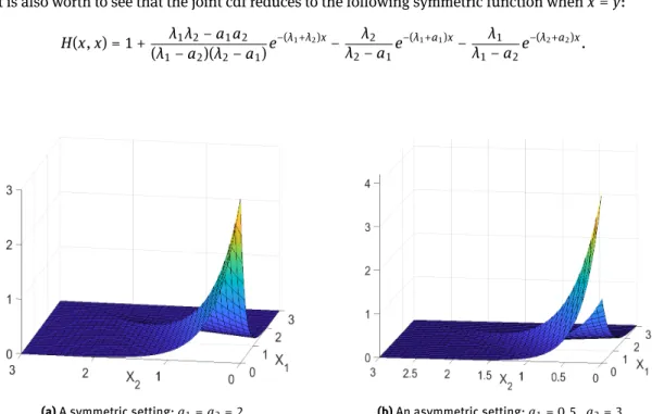
Figure 1 depicts the joint density function of (X1,X2) for two parameter settings.
All the cdfs and pdfs in formulas (3)–(13) continuously depend on the parametera1anda2. For instance,
this continuity is trivial for the marginal density functions (10) and (11) when a1≠ λ2 and a2 ≠λ1. At the
places a1 = λ2 resp. a2 = λ1 one can see the continuity by taking the limits a1 → λ2 anda2 → λ1 in
formula (10) and (11), which then yield formula (12) and (13).
Similarly, the special case of the joint cdf presented in (i) (b) can be also obtained from the general formula (3), if we leta2→λ1, since lim
a2→λ1 e−(λ1−a2)x− 1 λ1−a2 = −x, and lim a2→λ1 a2·e−(λ1+λ2)y−λ 1·e−(λ2+a2)y λ1−a2 = −e−( λ1+λ2)y−λ 1·y·e−(λ1+λ2)y.
The marginal density (10) reduces to f(x) = λ1·e−λ1x if a
1 = 0 , so in this case X1 is exponentially
distributed with parameter λ1. It might be surprising at first glance, when someone only considers the
con-struction (2) of X1. The background of this feature is the constant hazard rate property of the exponential
distribution. Nevertheless, a disturbance parameter a1 of value 0 has indeed no effect on the marginal
dis-tribution of the first entity, since in this case X1 ∼ Y1. However, X1 and X2 are not independent, unless a2= 0 also holds.
We examine the other extreme case as well, i.e., when a1→∞ . Then Z1a.s.= 0∼"Exp(∞)" is added to
the (truncated)Y1, which means finally that either the first entity expires earlier (Y1<Y2), or X1 takes the
value of Y2, so all in allX1= min{Y1,Y2}, which is exponentially distributed with parameterλ1+λ2. This
fact is also reflected by the marginal density f (look at (10)), which reduces to f(x) = (λ1+λ2) ·e−(λ1+λ2)x in this case.
It is also worth to see that the joint cdf reduces to the following symmetric function whenx=y: H(x,x) = 1 + λ1λ2−a1a2 (λ1−a2)(λ2−a1)e −(λ1+λ2)x− λ2 λ2−a1e −(λ1+a1)x− λ1 λ1−a2e −(λ2+a2)x. (14)
(a)A symmetric setting:a1=a2= 2. (b)An asymmetric setting:a1= 0.5,a2= 3.
Figure 1:Joint density of(X1,X2)for two different parameter settings.
We remark that the parameter constellationa1 = ∞, a2 = ∞ corresponds to the special case of the
Marshall-Olkin model, when λA = 0,λB = 0, λ{A,B} > 0, i.e., the system of two entities can face only a
common shock. (No separate individual shocks are present.)
Inverse marginal cumulative distribution functions.
Notice that the univariate quantile functions (i.e., the inverse functions of the marginal distribution functions (8), (9)) are smooth, but they cannot be written in a closed, analytical form (except in some very special cases). Since in this current work the quantile functions are mainly used in connection with the copula function, we will further elaborate this question in Subsection 2.3.
2.3 Copula function and copula density
We have discussed the features of the lifetimes variablesX1, X2, but in the end we are mainly interested in
their copula. While the lifetimes are given by the pair (X1, X2) , their copula is defined on the pair of uniform
marginals (U,V), whereU=F(X1), V=G(X2) and F,G are the marginal cdfs (8) and (9).
The copula function (15) and copula density (16) in our model – in accordance with the standard literature – are defined as follows.
C(u,v) =H(F−1(u),G−1(v)) for 0 ≤u, v≤ 1 , (15)
whereF−1(u) and G−1(v) are the generalized inverse functions of the cumulative distribution functions (8)
and (9), namely they are the true inverse functions for 0 ≤ u,v < 1 , and F−1(1) = ∞, G−1(1) = ∞ . The
copula density is given by
c(u,v) = ∂2C(u,v)
∂u∂v for (u,v)∈[0, 1]
2\{(1, 1)}. (16)
Notice that the formula (16), strictly speaking, cannot be extended to the entire [0, 1]2, since lim
(u,v)→(1,1)c(u,v) = ∞, i.e., the copula density is unbounded around (1, 1). To see the unboundedness, we provide a sketch of the argument. The details are left to the reader.
Notice first thatc(u,v) = ∂2C(u,v)
∂u∂v =h(F−1(u),G−1(v)) ·
∂F−1(u) ∂u ·
∂G−1(v)
∂v . The formulas
(8) and (9) show thatFandGare, roughly speaking, of typeF(x) ≈ 1 −α·e−β·xexpressions,
whereα> 0,β> 0. HenceF−1(u) ∂u ≈
1
β· (1 −u).
Similarly, one can argue that
h(F−1(u),G−1(v)) ≈
(
c1· (1 −u)κ1· (1 −v)κ2 if 0 ≤F−1(u) ≤G−1(v),
c2· (1 −v)κ3· (1 −u)κ4 if 0 ≤G−1(v) ≤F−1(u). whereκ1< 1,κ2≥ 1,κ3< 1,κ4≥ 1.
Altogether, the above considerations and formulas mean thatc(u,v) is unbounded whenboth u→1 and
v→1, and in all other cases it is bounded.
If one wishes to compute explicitly the copula function (15), then an explicit formula for the inverse marginal cumulative distribution functions F−1(u) , G−1(v) would be needed as well, but in our model this
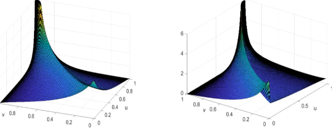
is impossible in most cases (look at (8) and (9)). Therefore we will use numerical methods, as the reader will see in the following. In Figure 2, the copula density is shown for a symmetric and for an asymmetric case.
(a)A symmetric setting:a1=a2= 2. (b)An asymmetric setting:a1= 0.5,a2= 3.
2.4 Scatter plots of copulas for different parameter settings
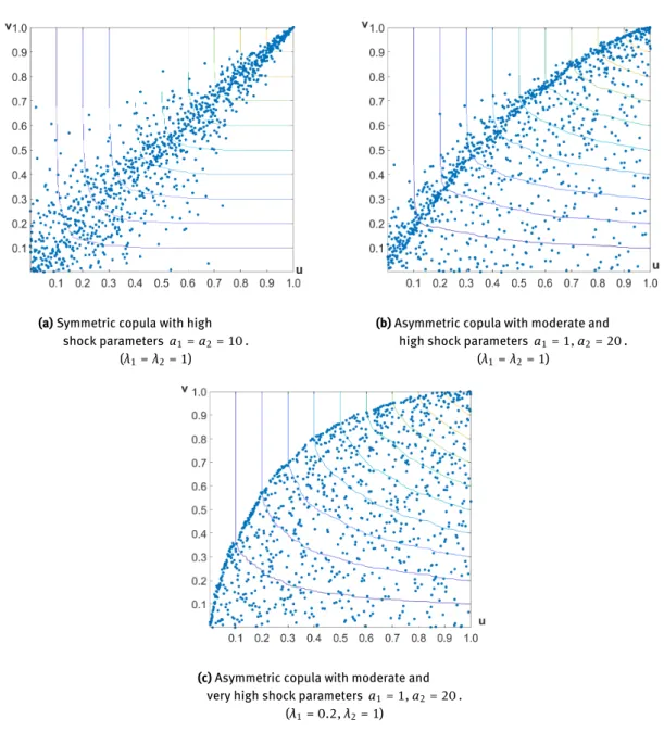
A great advantage of our model is the flexibility that it can easily handle asymmetric situations, too, i.e., when the effect of the default of an institution on another institution is larger than vice versa. Figure 3 gives an insight into the dependence structure by scatter plots, which are common tools for visualizing bivariate (or even three-variate) copulas.
(a)Symmetric copula with high shock parameters a1=a2= 10.
(λ1=λ2= 1)
(b)Asymmetric copula with moderate and high shock parameters a1= 1,a2= 20.
(λ1=λ2= 1)
(c)Asymmetric copula with moderate and very high shock parametersa1= 1,a2= 20.
(λ1= 0.2,λ2= 1)
Figure 3:Scatter plots of copulas for different parameter settings based on samples of size1000. The contour lines of the empirical copula functions for the values 0.1,. . ., 0.9are also shown.
In Figure 3b, we recognize a narrow region where many observations accumulate. We can call this a "line mass". Such a region is also present on Figure 3a and 3c, but the most visible on 3b. Notice that this line mass corresponds to the ridge which can be seen at the copula density plots (Figure (2a) and (2b)). Two questions arise: what is the interpretation of the line mass and which curve describes this line?
that in the case when Y1 expires earlier than Y2, the (new) remaining lifetime of the second entity will
be typically very short, since it follows an exponential distribution with parameter λ2+a2 = 21 . Loosely
speaking, it results inX1≈X2 (or if one wishes X1.X2), so this is the interpretation of the line mass. The
corresponding probability, i.e., the weight of the line mass, isP(X1≈X2) ≈P(Y1<Y2) = λ1 λ1+λ2 = 12.
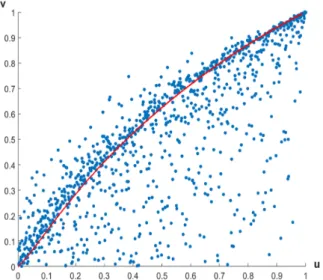
The theoretical equation of the curve of the line mass (see also Figure 4 ) is obtained by setting a2= ∞ ,
and then we can use the exact equalityX1=X2 (which event has probability 12 due to the above mentioned
fact), and then we obtainv(u) =G(F−1(u)) , where u andvare the variables of the copula function (see also
(15) ) .
Figure 4:Scatter plot of the copula of(X1,X2)with the limiting curvev(u) =G(F−1(u))of the "line mass". This curve corresponds to the parameter settingλ1=λ2= 1,a1= 2,a2= ∞; The scatter plot shows the empirical copula of a sample of
size 1000 from the modelλ1=λ2= 1,a1= 2,a2= 20.
It may be shown that this copula family does not exhibit the Archimedean property (for the definition of Archimedeanity look at for instance Nelsen [9]), since the associativity does not hold. The details of this analysis are omitted.
2.5 The idea of a multivariate setting
LetY1,. . .,Ynbe independent exponential random variables with Yk ∼ Exp(λk), k = 1,. . .,n. We con-struct the actual lifetime variables X(kq) (k = 1,. . .,n) for the q-th phase of an m-step cascading effect
(q = 1,. . .,m;m < n) via the following mechanism. Note that defining anm-step cascade in our model
means to define an orderedm-tuple of indices (k1,. . . km) which indicates the defaulting institution in each step.
For the first step (first phase) of the cascade let
Yk1 = min
1≤k≤nYk (17)
i.e., the institution that defaults first in a certain realization is denoted by k1. Let us introduce the variables Zk,k1 ∼Exp(λk+ak,k1) with parameters ak,k1 ∈[0, ∞) for k1≠k, and withak,k= ∞ . (In this latter case the
corresponding random variable is degenerated, namelyZk,k = 0 with probability 1 .) The variablesZk,k1are
independent of each other and of allYks. We define the modified lifetime variablesX(1)k (k= 1,. . .,n) via X(1)k :=Yk1+Zk,k1 for k= 1,. . .,n. (18)
The random variable Zk,k1, more precisely the shock parameter ak,k1, expresses the effect of the default of institution k1 on institution k.
We introduce the notation I1, the index set of defaulted institutions after one step of the cascade. With
this notation I1={k1}.
As already mentioned, the parameters can be organized as an×nmatrix. We always assume in this
paper that Zk,k= 0 with probability 1 for all k= 1,. . .,n, which corresponds to ak,k= ∞, i.e., there is no
possibility for governmental or other kind of bailout, when an institution has already defaulted. Note that the random variablesX(1)k are not exponentially distributed anymore (except when ak,l= 0, l= 1,. . .,n,l≠k
for some k), and also no longer independent (unless all ak,l= 0 for k≠l) .
After the first step of the cascading effect described in (17) and (18), the institutions continue operating until the next default happens. Let
X(1)k
2 =1≤kmin≤n,k≠k1X (1)
k (19)
i.e., the institution that defaults in the second step of the cascading effect is denoted by k2. Then X(2)k :=X(1)k
2 +Zk,I2 for k= 1,. . .,n, (20) where I2 = {k1,k2} is the set of defaulted institutions after two steps of the cascade, Zk,I2 = Zk,k1,k2 ∼
Exp(λk+ak,k1 +ak,k2), and the variables Zk,k1,k2 are independent of each other and also independent of
any other variables. The random variable Zk,k1,k2, more precisely the parameter ak,k1+ak,k2, expresses the effect of the defaults of institutions k1 and k2 on institution k. We also assume here (like in the first step)
that Zk,I2= 0 with probability 1 , when k∈I2.
Note that the setting in (20) does not distinguish the order of defaults regarding institutions k1 andk2.
Furthermore, by the definition of Zk,I2, we impose a simple and well-tractable additivity for modelling the effect of consecutive defaults.
Finally, to put it more generally, in theq-th step of the cascading effect (q= 1,. . .,m), let X(kq−1)
q = min1≤k≤n,
k∉Iq−1
X(kq−1), (21)
where Iq−1={k1,. . .,kq−1}is the index set of the already defaulted institutions. So we call (label) the insti-tution which defaults in the q-th phase bykq. (X(0)k =Yk for all k= 1,. . .,n andI0=∅. ) Then
X(q)k :=X(q−1)k
q +Zk,Iq for k= 1,. . .,n, (22)
where Zk,Iq ∼ EXP(λk+ P
p∈Iq
ak,p) , and the variables Zk,Iq are independent of each other and also
inde-pendent of any other variables. The random variable Zk,Iq, more precisely the parameter ak,k1+. . .+ak,kq,
expresses the effect of the defaults of institutions k1,. . .,kq on institution k. We also assume here that if
k∈ Iq, then Zk,Iq = 0 with probability 1 . (Similarly as we have stressed it after step (20), the order within
the index setIqin (22) does not play any role.)
We also emphasize that the index sets Iq (q = 1,. . .,m) are random in the sense that they depend on the particular realizations of the random variables X(kq−1) (k= 1,. . .,n).
3 Examining the change in the dependency structure in a
symmetric case
In this section, we consider the monotonicity properties of the copula for the symmetric model [λ,λ,a,a].
Notice that the copula is invariant with respect to scaling of the time axis, implying that the copulas of the models [λ,λ,a,a] and [1, 1,a/λ,a/λ] are identical.
The dependency structure between the lifetime variables X1,X2 is given by the joint cumulative
distri-bution function (3), or alternatively (but not equivalently) by the copula function (15). Both of them depend on four parameters (λ1,λ2,a1,a2). Our ultimate goal is to study how the joint cdf resp. the copula changes,
when we let these parameters vary.
We consider the joint cdf (23), the marginal cdfs (24), (25), the copula function (26), the joint density (27), and the marginal densities (28), (29) in this special case. These formulas are gained obviously by specializing the general formulas (10), (11), (5), (8), (9), (3) and (15).
The one-parametric setting is also reflected in the notation. First we list the functions fora≠ 1 in formulas
(23)–(29), then fora= 1 in formulas (30)–(35) .
Ha(x,y) = 1 + 1
1−a·e−(1−a)x·e−(1+a)y+1−aa ·e−2x− 1−a1 ·e−(1+a)x−1−a1 ·e−(1+a)y if 0 ≤x≤y, 1 + 1 1−a·e−(1−a)y·e−(1+a)x+1−aa·e−2y−1−1a·e−(1+a)y−1−1a·e−(1+a)x if 0 ≤y≤x. (23) Fa(x) = 1 − 11 − a·e −(1+a)x+ a 1 −a·e −2x. (24) Ga(y) = 1 − 1 1 −a·e −(1+a)y+ a 1 −a·e −2y. (25) Ca(u,v) =Ha(F−1a (u),G−1a (v)) for 0 ≤u,v≤ 1 . (26) ha(x,y) = (a+ 1) ·e−(x+y)−a·|x−y| x≥ 0, y≥ 0 . (27) fa(x) = − 2a 1 −a·e −2x+ 1 +a 1 −a·e −(1+a)·x x≥ 0 . (28) ga(y) = − 2a 1 −a·e −2y+ 1 +a 1 −a·e −(1+a)·y y≥ 0 . (29) H1(x,y) = ( 1 −x·e−2y− (x+ 1) ·e−2x if 0 ≤x≤y, 1 −y·e−2x− (y+ 1) ·e−2y if 0 ≤y≤x. (30) F1(x) = 1 − (x+ 1) ·e−2x if x≥ 0. (31) G1(x) = 1 − (y+ 1) ·e−2y if y≥ 0. (32) h1(x,y) = 2 ·e−2·max{x,y} x≥ 0, y≥ 0 . (33) f1(x) = (2x+ 1) ·e−2x x≥ 0 . (34) g1(x) = (2y+ 1) ·e−2y y≥ 0 . (35)
We will examine the change in the dependency structure given by (23)–(29) in two different ways. First we will consider some indicators (like expectation, variance, correlation coefficients of several kinds, etc.) extracted from the bivariate distribution. We will present these in Subsection 3.1. Secondly, we attempt to catch the dependency structure as a whole, and in Subsection 3.2 we will prove monotonicity result in the upper orthant order as parametera varies.
3.1 Dependence measures
Figure 5:Three usual correlation coefficients for(X1,X2).
In this subsection we will examine the most common correlation coefficients studied in the literature, namely the usual product moment correlation (also known as Pearson’s correlation coefficient), Spearman’s
ρ and Kendall’s τ. As Figure 5 shows, each of them is increasing function of the model parameter a. We
provide analytic formulas for the (Pearson’s) correlation and for Spearman’s ρ(see also Figure 5), from which
the increasing property can be clearly verified. It seems impossible for us to derive an analytic formula for Kendall’sτ(we will explain the reason for that in the corresponding paragraph). However, by sampling from
our model and by numerically evaluating Kendall’sτfor the samples, we obtained a curve for it. Furthermore,
the increasing property of Kendall’s τ will be proved in Proposition 2.
Expectation, variance, covariance and correlation.
Since the marginal densities (28), (29) and the joint density (27) are simply sums of exponential functions, we get by elementary calculus that
Ea(X1) =Ea(X2) = 12 ·a+ 2 a+ 1 and Ea(X1·X2) = 12 + 1 2 ·a1+ 1, consequently cova(X1,X2) = a· (a+ 2) 4 · (a+ 1)2.
The variance ofX1(and ofX2) is
D2a(X1) = 14 ·(
a+ 1)2+ 3
(a+ 1)2 , therefore corra(X1,X2) =
a(a+ 2)
(a+ 1)2+ 3.
The previous formulas show that fora= 0 thecovarianceand thecorrelationofX1andX2 is 0 . It is also
obvious from the more general fact that they are independent, which can be seen by substituting a1=a2= 0
in the general formula (5) of the joint density function.
The formulaEa(X1) =Ea(X2) =12·aa+2+1 has a nice interpretation as a→∞ . In this case, the realizations of the two lifetime variables differ less and less from each other, and their marginal distributions can be approximated better and better with min{Y1,Y2}, which is distributed according toExp(λ1+λ2) , i.e., in our
case Exp(2) .
We can also see that cova(X1,X2)→14 as a→∞ . It is more informative to examine the limit of the correlation: corra(X1,X2)→1 as a→∞ .
Spearman’s ρ.
For (bivariate) samples Spearman’s ρ is defined through the order statistics, namely the correlation of
the ranked data. Accordingly, for distributions we need to compute the following (in notation we immediately use our variables):
ρa= cov(U,V)
D(U) ·D(V) = 12 · Ea(U·V) −Ea(U) ·Ea(V)
= 12 ·Ea(U·V) − 3.
Using the fact thatU=F(X),V =G(Y), and formulas (24), (25) and (27) consist of (sums of) exponential
functions, through a cumbersome, but elementary computation we get that Ea(U·V) = ∞ Z 0 ∞ Z 0 Fa(x) ·Ga(y) ·ha(x,y)dx dy= 13 ·2a 3+ 20a2+ 54a+ 45 2a3+ 20a2+ 62a+ 60. Finally we getρa= 4· 2a 3+ 20a2+ 54a+ 45 2a3+ 20a2+ 62a+ 60−3 = 2a3+ 20a2+ 30a
2a3+ 20a2+ 62a+ 60, which is pictured in Figure 5 .
Kendall’s τ.
Recall that for a bivariate general copulaC, Kendall’sτis defined as τ= 4 · 1 Z 0 1 Z 0
C(u,v)dC(u,v) − 1. If the copula is the empirical one based on a sample
(X1(i),X2(i))Ni=1, then Kendall’s τ can be also defined as
τ = # concordant pairs − # discordant pairs
N 2
.
(A pair (X1(i),X2(i)) is called concordant with another pair (X1(j),X2(j)), if sgn(X1(i) −X1(j)) = sgn(X2(i) − X2(j)), otherwise they are discordant.)
Now we are ready to present the increasing property of Kendall’sτin Proposition 2. Then the reader finds
the main result of this paper in Proposition 3, namely the upper orthant ordering concerning the copulasCa. We notice that by Theorem 5.1.9 in Nelsen [9], Proposition 2 is a direct consequence of Proposition 3. We still present them in this order, because the proof of Proposition 2 only focuses on (concordant) pairs in a sample, while the proof of Proposition 3 deals with the entire order statistics, and in this way it can be considered as an extension of the proof of Proposition 2.
Proposition 2.
Let τa be Kendall’s τ pertaining to the copula model [1, 1,a,a]. Then a 7→ τa is monotonically non-decreasing.
Proof.
Consider an i.i.d. sampleSaN =
(X1a(i),Xa2(i)) N
i=1according to the model [1, 1,a,a]. Such a sample can be generated by the following algorithm: LetU(i) and V(i) be the realizations of independent Uniform[0,1]
variables fori= 1,. . .,N. Then
• with probability 1/2 Xa1(i) = −12 log(U(i)); Xa2(i) = −12 log(U(i)) − 1 1 +alog(V(i)), • with probability 1/2 Xa2(i) = −12 log(U(i)); X1a(i) = −12 log(U(i)) − 1 1 +alog(V(i)).
For a given sampleSaN, let U = {i : Xa1(i) < Xa2(i)} and L = {i : Xa1(i) > Xa2(i)}. Notice that the event
Xa1(i) =X2a(i) has probability zero. Notice now that ifZ∼Exp(1 +a), then 1+1+aa0 ·Z∼Exp(1 +a0). Therefore
we can easily modify the sampleSaNto get a valid sampleSaN0 =n(X1a0(i),Xa20(i))oN
i=1for model [1, 1,a 0,a0]. To this end, let
• fori∈L X1a0(i) =Xa2(i) + (Xa1(i) −Xa2(i)) · 1 +a 1 +a0; X a0 2 =X2a, (36) • fori∈U X2a0(i) =Xa1(i) + (Xa2(i) −Xa1(i)) · 1 +a 1 +a0; X a0 1 =X1a. (37)
We claim that the number of concordant pairs in sampleSaN0 is not less than the number of
concor-dant pairs in sampleSaN. To prove this assertion, let (i,j) be a concordant pair inSaN, i.e., X1a(i) −X1a(j)
·
X2a(i) −X2a(j)
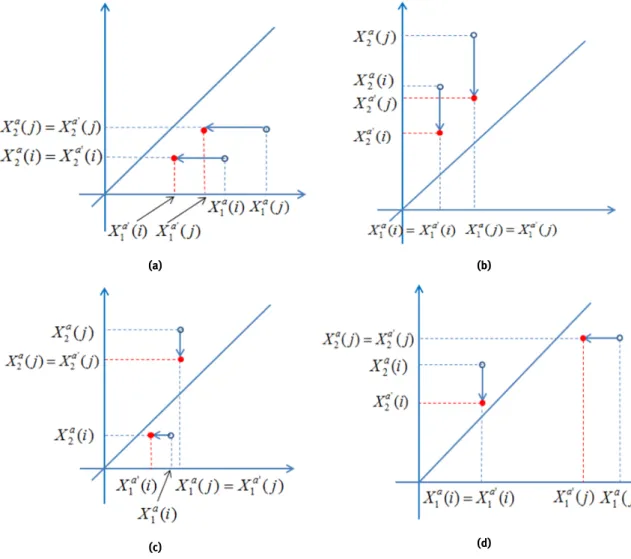
> 0. We now have to distinguish four cases: (a), (b), (c) and (d) . (a) Xa1(i) >Xa2(i) , Xa1(j) >Xa2(j) ,
(b) Xa1(i) <Xa2(i) , Xa1(j) <Xa2(j) ,
(c) Xa1(i) >Xa2(i) , Xa1(j) <Xa2(j) ,
(d) Xa1(i) <Xa2(i) , Xa1(j) >Xa2(j) .
We have illustrated the situation in Figure 6, where the original pairs (X1a(i),X2a(i)) and
(Xa1(j),Xa2(j)) are shown as little circles ◦ and the modified pairs (X1a0(i),X2a0(i)) and
(Xa10(j),Xa20(j)) are shown as dots•.
(a) (b)
(c) (d)
Figure 6:The four possible positions of a concordant pair(i,j)(marked by◦). The transformed sample (marked by•). Concordant pairs remain concordant.
W.l.o.g. we may assume that Xa1(j) −Xa1(i) > 0 and X2a(j) −X2a(i) > 0 . Let us look e.g., at case (a). Here Xa10(j) −Xa10(i) = a 0−a 1 +a0 · X a 2(j) −Xa2(i)+ 1 +1 +aa0 · X a 1(j) −Xa1(i)> 0 , and X2a0(j) =Xa2(j) , Xa20(i) =X2a(i) , so X2a0(j) −X2a0(i) =Xa2(j) −Xa2(i) > 0 .
In case (b) only the roles of the coordinates are exchanged. In case (c) we have
Xa10(i) <Xa1(i) <Xa1(j) =X1a0(j)
and
X2a0(i) =X2a(i) <Xa1(i) <Xa1(j) =X1a0(j) <X2a0(j) .
The last inequality holds, because the point (X1a0(j),X2a0(j)) lies above the diagonal line y=x. Again,
inter-changing the roles of the coordinates shows also the validity of the statement in case (d).
Finally, we argue that the empirical copula converges a.s. to the true one (see e.g., Gaensslar and Stute [5]) and that the empiricalτconverges to the trueτ. Thus we obtain the statement.
3.2 Monotonicity of the copula in upper orthant order w.r.t. parameter
a
Our general purpose is to examine how the copula (26) (and slightly more general the copula (15) for the model [λ,λ,a,a] ) changes as we change the value of parametera, i.e., to determine and describe (some properties
of) the functiona7→Ca.
Upper orthant order for copulas.
Definition 1. LetC1andC2 be two bivariate copulas and let (U1,V1) be distributed according toC1and
(U2,V2) be distributed according toC2. We say thatC1is dominated byC2in upper orthant order (in symbol C1UOC2), if
P(U1>u,V1>v) ≤P(U2>u,V2>v)
for allu,v∈[0, 1]. In other words one may say thatC2is more (co-monotone) dependent thanC1.
Remark 1. SinceP(U≤u,V≤v) = 1 −u−v+P(U>u,V >v), one sees that thatC1UOC2is equivalent to
C1(u,v) ≤C2(u,v) (38)
for all u,v∈[0, 1] .
Some authors say that the random vector (U2,V2) is smaller than the random vector (U1,V1) in lower
orthant order, if (38) holds (see e.g., Denuit et al. [3], Definition 3.3.80). Nevertheless, the notion of lower orthant order is not needed in our work.
We now formulate the main result of this section.
Proposition 3. LetCa(u,v) be the copula of the model [1, 1,a,a] and letCa0(u,v) the copula of the model
[1, 1,a0,a0], wherea≤a0. Then
CaUOCa0. (39)
Proof.We have to show thatCa(u,v) ≤Ca0(u,v) for allu,v. We use the same construction for the samplesSa
N resp.SaN0as in the proof of Proposition 2. (Look at (36) and (37).)
Notice that for alls,t
#{i:Xa1(i) ≤s,X2a(i) ≤t}≤ #{i:Xa10(i) ≤s,X2a0(i) ≤t}.
We will show first that for the empirical copulaC(aN)of the sample (X1a(i),X2a(i)),i= 1,. . .,Nwe have the upper orthant order
for allu,v∈[0, 1].
LetXa1[i: N] andXa2[j: N] be the order statistics and letXa1(`1a) = Xa1[i: N] andXa2(`a2) =Xa2[j: N]. For u=i/N,v=j/Nwe set
Ia={i:Xa1(i) ≤Xa1(`1a);X2a(i) ≤Xa2(`2a)}
andma= #(Ia). Notice thatC(aN)(u,v) =ma/N. We have to show thatmais monotonically increasing witha. We may assume w.l.o.g. that there are no ties in the sample. If the index setsIado not change for some a0 >a, the empirical copula also does not change. Let nowa0be such that exactly one index changed from IatoIa0, because one of the the indices`a1,`2achanged. Suppose for instance thatXa10(`a1) is no longer thei-th
largest among theXa10(.), but there is a`0∉Iasuch thatX1a0(`0) <X1a0(`a1). Then two situations may occur: • IfXa20(`0) >X2a0(`a2), thenma0=ma.
• IfXa20(`0) ≤X2a0(`a2), thenma0 =ma+ 1.
In both cases ismanon-decreasing. One may repeat the argument for two indices changing, three indices
changing and so on to see that (40) is proved. Now, again invoking the argument that the empirical copulas converge to the true copulas as in Proposition 2, one sees that
Ca(u,v) ≤Ca0(u,v)
holds for allu,v∈[0, 1] .
Corollary.
Recall that Blomqvist’sβfor the copulaCis defined asβ= C(1/2, 1/2) (see Blomqvist [1]). As a
conse-quence of Proposition 3 also this correlation coefficient is monotonic ina, i.e., the function a7→βa=Ca(1/2, 1/2)
is monotonically increasing.
4 An application for measuring systemic risk
It is a usual approach in financial theory and practice that the strength and vulnerability of the institutions is quantified by indirect manners. This is because an actual default or bankruptcy of a financial institution occurs very rarely, however the stability of the institutions can vary significantly. In this way, the lifetime model presented in Sections 1, 2 and 3 can also be considered as an indirect tool to measure the stability and potential strength of entities in a financial system.
In this section we have two aims. First, we relate our lifetime variables to loss variables, since mostly these latter ones are in the focus of interest for financial institutions. Secondly, we also establish a relation between lifetime intensities and CDS spreads, which are widely used indicators for the financial strength of entities in banking systems. This enables us to provide numerical illustration for our model using real financial data.
We will formulate the definitions for arbitraryn, and in the numerical case study we will restrict our
analysis ton= 2 .
4.1 Relation between lifetime and loss variables; a model for systemic risk
In the previous sections, we dealt with defining and exploring a joint lifetime model, where we considered the random vector of lifetimes (X1,. . .,Xn) . In this subsection, we translate the distribution of lifetimes into the distribution of losses, so we introduce the random vector of losses (L1,. . .,Ln) . The basic idea is simple: the longer the lifetime is, the less the losses are. There are several ways how to formulate this. In the following we list a few of them.
A few possible definitions of loss variables defined via lifetime variables. (i) Li:= min 1 Xi, c , (i= 1,. . .,n), wherec> 0 is a constant. (ii) Li:=ci·e−r·Xi, (i= 1,. . .,n), where c
iis the initial capital of institutioni, and ris the risk-free interest rate.
(iii) Li:=1{Xi≤ti}, (i= 1,. . .,n), whereti> 0 is a threshold.
(iv) Li:=
(
ξi ifXi≤ti,
0 ifXi>t, (i= 1,. . .,n), whereti > 0 is a threshold, andξiis a random variable with given
distribution.
Quantifying systemic risk.
While the individual risk refers to the fact that random losses may occur to a financial institution, the notion of systemic risk measures the extra risk which can be attributed to the interdependence of several institutions. LetRbe a risk functional, which assigns a real value to the risk of a potential loss variableL. If
the system consists ofninstitutions, thenL1+. . .+Lnis the total loss of the whole system. The distribution of this sum depends on the marginal distributions and the copula. For fixed marginal distribution, let us write
M
a C
Li
for the total loss variable, when the individual losses are coupled by copulaC.
Definition 2. (See also Pflug and Pichler [10]). For a given risk functionalR, define the systemic risk by
R(C,R;L) =R M a C Li −R M a Π Li , (41)
whereL= (L1,. . .,Ln) is the vector of (univariate) marginal loss variables andΠis the independent copula. (41) compares the total loss under the copulaCwith the (hypothetical) total loss of independent institutions.
In particular, one may considerCas the copula of the lifetimes (X1,. . .,Xn) (e.g., a Freund copula) and losses depending on the lifetimes via the above formulas (i)–(iv).
In Definition 3 we recall the notion of average-value-at-risk, which can be found in several sources, e.g., in Pflug and Römisch [11]. We would like to stress that technically there are two variants of theAV@R, the lower-AV@R, which focuses on the left tail of the distribution, and the upper-AV@R, which focuses on the right
tail. We will need this latter one.
Definition 3. LetXbe a random variable with cdfF, and let 0 ≤α< 1. The (upper) average-value-at-risk at
levelαis defined as AV@Rα(X) = 1 1 −α 1 Z α F−1(u)du, (42)
whereF−1(u) is the generalized inverse function ofF.
Remark 2. When it is clear from the context which significance levelαis meant, or a certain statement holds
for allα, then the lower index can be omitted from the notation, and we simply writeAV@R(X).
Remark 3. It was shown in Pflug and Pichler [10] thatC1UOC2implies that
AV@R M a C1 Li ≤AV@R M a C2 Li . In particular, by Proposition 3, for our bivariate copulaCa(26) we have that
AV@R(L1⊕a Ca
L2) ≤AV@R(L1⊕a Ca0
fora≤a0.
Notice also that if a1 = a2 = 0 in our model, thenR = 0, so the system does not possess any systemic
risk. It does not mean that the overall risk in the system would be zero, but it means that the part of the risk, which is attributed only to the dependencies of the institutions, is zero.
Examples.
We illustrate our systemic risk definition through some examples. For the sake of simplicity we consider in each of these examples the model
[1, 1,a1,a2]. (43)
Example 1. Let (X1,X2)∼H, whereHis according to (3), specified by (43).
To define the relation between lifetimes and losses we will use (i) from the list above. Let us assume that both institutions have capitalc= 10 (units).
SoL1= min(1/X1, 10),L2= min(1/X2, 10).
For the risk functionalRlet us chooseR(L) := E(L−t|L > t), whereLis a loss variable, andtis a threshold, whose excess is considered as a "bad" event. This risk functional is closely related to thestop-loss
transform, which is a popular risk functional in insurance mathematics (look at for instance Denuit et al. [3], Definition 1.7.1.1) . In accordance with our systemic risk definitionL:=L1+L2, and let us set the threshold t = 10 . It means that we consider a situation risky, when the market loses half of its capital or more. The
following table shows for some values how the systemic riskR(C,R;L) (see Definition 2) increases as we
increase the shock parameters a1,a2.
(a1,a2) (0,0) (0,1) (1,1) (1,3) (2,3) (5,5) (10,10) (100,100)
R(⊕CLi) 2.2810 2.7831 3.2644 3.8351 4.1676 5.0480 5.8924 7.2118
R(C,R;L) 0 0.5021 0.9834 1.5541 1.8866 2.7670 3.6114 4.9308
rel.incr. 0% 22.01% 43.11% 68.13% 82.71% 121.31% 158.33% 216.17%
The fourth line of the table shows the relative increment in the systemic risk, compared to the independent case.
Example 2. Let (X1,X2) ∼ H, whereH is according to (3), specified by (43). Let us define now the loss
variables according to (ii) from the above list, i.e., viaL1=c1·e−r·X1andL
2=c2·e−r·X2, wherec1=c2 ..= 1, and the risk-free interest rateris set up tor= 0.05.
The risk functional is defined as in Example 1, with thresholdt= 1.
We can observe again the increase in systemic risk as we increase the shock parametersa1,a2, but in a
much more moderate way.
(a1,a2) (0,0) (0,1) (1,1) (1,3) (2,3) (5,5) (10,10) (100,100)
R(⊕CLi) 1.9049 1.9163 1.9275 1.9334 1.9373 1.9432 1.9466 1.9508 R(C,R;L) 0 0.0114 0.0226 0.0285 0.0324 0.0383 0.0417 0.0459
rel.incr. 0% 0.59% 1.19% 1.49% 1.70% 2.01% 2.19% 2.41%
Example 3. Let (X1,X2) ∼ H, whereH is according to (3), specified by (43). Let us define now the loss
variables according to (iii) from the above list, i.e., viaLi=1{Xi≤ti}, whereti:=Q
(Xi)
0.8 ( 0.8-quantile ofXi) for
i= 1, 2.
For the risk functional let us chooseR(L) =AV@R(L), i.e., in the light of Definition 2 R(L1+L2) =AV@R0.8(L1+L2) .
(a1,a2) (0,0) (0,1) (1,1) (2,3) (5,5) (10,10)
R(⊕CLi) 1.200 1.2895 1.4665 1.6305 1.8020 1.8950 R(C,R;L) 0 0.0895 0.2665 0.4305 0.6020 0.6950
rel.incr. 0% 7.46% 22.21% 35.88% 50.67% 57.92%
Example 4. Let (X1,X2) ∼ H, whereH is according to (3), specified by (43). Let us define now the loss
variables according to (iv) from the above list, i.e., via
Li=
(
ξi ifXi≤t
0 ifXi>t
i= 1, 2, whereξi∼Exp(1) independent ofX1andX2.
The threshold is set up to t= 1.3863, that is the 75%-quantile of theExp(1) distribution, i.e., the
distribu-tion ofX1 and ofX2, when a1=a2= 0 .
The risk functional is defined again as in Example 1.
A survey of the numerical study can be seen in the following table.
(a1,a2) (0,0) (0,1) (1,1) (1,3) (2,3) (5,5) (10,10) (100,100)
R(⊕CLi) 1.4996 1.6020 1.7024 1.7584 1.7954 1.8457 1.8599 1.8765 R(C,R;L) 0 0.1024 0.2028 0.2588 0.2958 0.3461 0.3603 0.376
rel.incr. 0% 6.82% 13.52% 17.26% 19.73% 23.08% 24.03% 25.07%
4.2 Numerical study using CDS-data
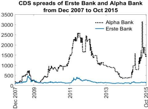
We use CDS-spread data, provided by the Data Centre of the University of Vienna. The data is on a daily basis, and consists ofN= 1907 observations of 77 banks from Europe and North-America on the time horizon Dec
2007 - October 2015. We will denote this data set by{s(i)}Ni=1, while for the CDS-spread as a (financial) variable
we use the notations.
The lifetime model presented above enables us to perform a numerical case study for pairs of institu-tions, which are very reduced subsystems of the entire data set. In spite of this, we believe that the following numerical illustration is informative enough, and convinces the reader that our model works.
Let us consider two banks from the above mentioned data set, Erste Bank (AT) and Alpha Bank (GRE). These are known to be different in financial strength and stability, therefore they seem to be a reasonable choice for our example.
Relation between CDS-spreads, lifetime variables and loss variables.
It is clear from the previous considerations that CDS-spreads are directly observable and given quantities. In order to apply our model, from these spreads we have to produce lifetime variables, which are in this sense artefacts.
From CDS spreads to lifetimes.IfXis the lifetime variable of the debtor of a CDS with spreadsand
maturityT, then the benefit is given by s min(X,T) Z 0 e−rtdt= s r(1 −e −rmin(X,T))
and the costs are
Figure 7:CDS spreads of Erste Bank and Alpha Bank given in basis points
HereLGDis the so-called (relative) Loss-Given-Default andris the interest rate. (In financial applications LGDis a commonly used notion, which expresses the maximal proportion of the firm’s capital, which can be
lost in case of default.)
For simplicity, we assume that the credits are long-term and setT= ∞. Equating the costs and the benefits
in this case one gets the relationship
X= −1 rlog s LGD·r+s . (44)
Now, in order to set up a data set for lifetime data, to each CDS-spread observation{s(i)}Ni=1of a certain
in-stitution we create an observation{X(i)}Ni=1using (44). (Note that the argumentirefers to the ordinal number
of the observation, as it was also the case in the proof of Proposition 2 and Proposition 3.)
X(i) = −1 r · log s(i) LGD·r+s(i) , (45)
whereLGDis the Loss-Given-Default andris the risk-free interest rate. In our analysisLGD= 0.5,r= 0.05.
In Subsection 4.1 we already discussed some alternatives how to link lifetime and loss variables. Consider now (ii) from the list in Subsection 4.1, i.e.,
L:=e−r·X. (46)
Combining (44) and (46) we obtain
L:= s
LGD·r+s, (47)
with which we gained one possible way for having a direct connection between CDS-spreads and losses, i.e., between the available inputs and objects of interest. Notice that the functionLgiven by (47) is a
monoton-ically increasing function. This implies that the spreads and the losses have exactly the same copula. Notice, however, that the copula of the lifetimes is the survival copula of the spreads: ¯C(u,v) = 1 −u−v+C(u,v),
but monotonicity w.r.t. parameterais preserved betweenCand ¯C.
Parameter estimation.
Our next task is to estimate the model parametersλ1,λ2,a1,a2, i.e., to find the copula in our model which fits