Generating functions for generating trees
Cyril Banderier, Philippe Flajolet, Dani`
ele Gardy, Mireille Bousquet-M´
elou,
Alain Denise, Dominique Gouyou-Beauchamps
To cite this version:
Cyril Banderier, Philippe Flajolet, Dani`ele Gardy, Mireille Bousquet-M´elou, Alain Denise, et al.. Generating functions for generating trees. Discrete Mathematics, Elsevier, 2002, 246 (1-3), pp.29-55. <hal-00003258>
HAL Id: hal-00003258
https://hal.archives-ouvertes.fr/hal-00003258
Submitted on 10 Nov 2004
HAL is a multi-disciplinary open access archive for the deposit and dissemination of sci-entific research documents, whether they are pub-lished or not. The documents may come from teaching and research institutions in France or abroad, or from public or private research centers.
L’archive ouverte pluridisciplinaire HAL, est destin´ee au d´epˆot et `a la diffusion de documents scientifiques de niveau recherche, publi´es ou non, ´emanant des ´etablissements d’enseignement et de recherche fran¸cais ou ´etrangers, des laboratoires publics ou priv´es.
ccsd-00003258, version 1 - 11 Nov 2004
Generating functions
for generating trees
Cyril Banderier Mireille Bousquet-M´elou∗ Alain Denise Philippe Flajolet Dani`ele Gardy Dominique Gouyou-Beauchamps
This article corresponds, up to minor typo corrections, to the article submitted to Discrete Mathematics (Elsevier) in Nov. 1999, and published in its vol. 246(1-3), March 2002, pp. 29-55. This work supplants a preliminary draft “On Generating Functions of Generating Trees” dated Nov. 1998 which appeared in the Proceedings of the FPSAC’99 Barcelona Conference.
Abstract
Certain families of combinatorial objects admit recursive descriptions in terms of gen-erating trees: each node of the tree corresponds to an object, and the branch leading to the node encodes the choices made in the construction of the object. Generating trees lead to a fast computation of enumeration sequences (sometimes, to explicit formulae as well) and provide efficient random generation algorithms. We investigate the links between the structural properties of the rewriting rules defining such trees and the rationality, algebraicity, or transcendence of the corresponding generating function.
1
Introduction
Only the simplest combinatorial structures — like binary strings, permutations, or pure invo-lutions (i.e., involutions with no fixed point) — admit product decompositions. In that case, the set Ωnof objects of sizenis isomorphic to a product set: Ωn∼= [1, e1]×[1, e2]×· · ·×[1, en].
Two properties result from such a strong decomposability property: (i) enumeration is easy, since the cardinality of Ωnise1e2· · ·en; (ii) random generation is efficient since it reduces to a
sequence of random independent draws from intervals. A simple infinite tree, called auniform generating tree is determined by theei: the root has degreee1, each of itse1 descendants has
degree e2, and so on. This tree describes the sequence of all possible choices and the objects
of size n are then in natural correspondence with the branches of length n, or equivalently with the nodes of generation nin the tree. The generating tree is thus fully described by its root degree (e1) and by rewriting rules, here of the special form,
(ei);(ei+1) (ei+1) · · ·(ei+1)≡(ei+1)ei,
where the power notation is used to express repetitions. For instance binary strings, permu-tations, and pure involutions are determined by
S : [(2), (2);(2) (2)] P : [(1), {(k);(k+ 1)k}
k≥1]
I : [(1), {(2k−1);(2k+ 1)2k−1}k≥1].
A powerful generalization of this idea consists in considering unconstrained generating trees where any set of rules
Σ = [(s0), {(k);(e1,k) (e2,k) · · ·(ek,k)}] (1)
is allowed. Here, the axiom (s0) specifies the degree of the root, while the productions ei,k
list the degrees of the k descendants of a node labeled k. Following Barcucci, Del Lungo, Pergola and Pinzani, we call Σ anECO-system(ECO stands for “Enumerating Combinatorial Objects”). Obviously, much more leeway is available and there is hope to describe a much wider class of structures than those corresponding to product forms and uniform generating trees.
The idea of generating trees has surfaced occasionally in the literature. West introduced it in the context of enumeration of permutations with forbidden subsequences [27, 28]; this idea has been further exploited in closely related problems [6, 5, 12, 13]. A major contribution in this area is due to Barcucci, Del Lungo, Pergola, and Pinzani [4, 3] who showed that a fairly large number of classical combinatorial structures can be described by generating trees.
A form equivalent to generating trees is well worth noting at this stage. Consider thewalks on the integer half-line that start at point (s0) and such that the only allowable transitions are those specified by Σ (the steps corresponding to transitions with multiplicities being labeled). Then, the walks of lengthnare in bijective correspondence with the nodes of generation nin the tree. These walks are constrained by the consistency requirement of trees, namely, that the number of outgoing edges from pointk on the half-line has to be exactly k.
Example 1. 123-avoiding permutations
The method of “local expansion” sometimes gives good results in the enumeration of per-mutations avoiding specified patterns. Consider for example the set Sn(123) of permuta-tions of length n that avoid the pattern 123: there exist no integers i < j < k such that
σ(i) < σ(j) < σ(k). For instance, σ = 4213 belongs to S4(123) but σ = 1324 does not, as
σ(1)< σ(3)< σ(4).
Observe that if τ ∈ Sn+1(123), then the permutation σ obtained by erasing the entry
n+ 1 fromτ belongs toSn(123). Conversely, for everyσ∈Sn(123), insert the valuen+ 1 in each place that gives an element ofSn+1(123) (this is the local expansion). For example, the permutation σ = 213 gives 4213, 2413 and 2143, by insertion of 4 in first, second and third place respectively. The permutation 2134, resulting from the insertion of 4 in the last place, does not belong to S4(123). This process can be described by a tree whose nodes are the permutations avoiding 123: the root is 1, and the children of any nodeσ are the permutations derived as above. Figure 1(a) presents the first four levels of this tree.
Let us now label the nodes by their number of children: we obtain the tree of Figure 1(b). It can be proved that the k children of any node labeled k are labeled respectively k+ 1,2,3, . . . , k (see [27]). Thus the tree we have constructed is the generating tree obtained from the following rewriting rules:
[(2), {(k) ;(2)(3). . .(k−1)(k)(k+ 1)}k≥2].
The interpretation of this system in terms of paths implies that 123-avoiding permuta-tions are equinumerous with “walks with returns” on the half-line, themselves isomorphic to Lukasiewicz codes of plane trees (see, e.g., [26, p. 31–35]). We thus recover a classic result [18]: 123-avoiding permutations are counted by Catalan numbers; more precisely, |Sn(123)|= 2n
n
1 21 12 321 231 213 312 132 4321 3241 3421 3214 4231 2431 2413 4213 2143 4312 3412 3142 4132 1432 5 2 3 4 3 2 4 2 3 4 2 3 3 2 4 2 3 3 2 3 2 2 (a) (b)
Figure 1: The generating tree of 123-avoiding permutations. (a) Nodes labeled by the per-mutations. (b) Nodes labeled by the numbers of children.
We shall see below that (certain) generating trees correspond to enumeration sequences of relatively low computational complexity and provide fast random generation algorithms. Hence, there is an obvious interest in delineating as precisely as possible which combinatorial classes admit a generating tree specification. Generating functions condense structural infor-mation in a simple analytic entity. We can thus wonder what kind of generating function can be obtained through generating trees. More precisely, we study in this paper the connections between the structural properties of the rewriting rules and the algebraic properties of the corresponding generating function.
We shall prove several conjectures that were presented to us by Pinzani and his coauthors in March 1998. Our main results can be roughly described as follows.
— Rational systems. Systems satisfying strong regularity conditions lead to rational gen-erating functions (Section 2). This covers systems that have a finite number of allowed degrees, as well as systems like (2.a), (2.b), (2.c) and (2.d) below where the labels are constant except for a fixed number of labels that depend linearly and uniformly onk. — Algebraic systems. Systems of a factorial form, i.e., where a finite modification of the
set {1, . . . , k} is reachable from k, lead to algebraic generating functions (Section 3). This includes in particular cases (2.f) and (2.g).
— Transcendental systems. One possible reason for a system to give a transcendental series is the fact that its coefficients grow too fast, so that its radius of convergence is zero. This is the case for System (2.h) below. Transcendental generating functions are also associated with systems that are too “irregular”. An example is System (2.e). We shall also discuss the holonomy of transcendental systems (Section 4).
Example 2. A zoo of rewriting systems
Here is a list of examples recurring throughout this paper.
[(3),{(k) ;(3)k−3(k+ 1)(k+ 2)(k+ 9)}] (2.a) [(3),{(k) ;(3)k−1(3k+ 6)}] (2.b) [(2),{(k) ;(2)k−2(2 + (kmod 2))(k+ 1)}] (2.c) [(2),{(k) ;(2)k−2(3−(kmod 2))(k+ 1)}] (2.d) [(2),{(k) ;(2)k−2(3−[∃p:k= 2p])(k+ 1)}] (2.e) [(2),{(k) ;(2)(3). . .(k−1)(k)(k+ 1)}] (2.f) [(1),{(k) ;(1)(2). . .(k−1)(k+ 1)}] (2.g) [(2),{(k) ;(2)(3)(k+ 2)k−2}] (2.h)
(In (2.e), we make use of Iverson’s brackets: [P] equals 1 ifP is true, 0 otherwise.) 2
Notations. From now on, we adopt functional notations for rewriting rules: systems will
be of the form
[(s0), {(k);(e1(k)) (e2(k)). . .(ek(k))}]
wheres0 is a constant and eachei is a function ofk. Moreover, we assume that all the values
appearing in the generating tree are positive: each node has at least one descendant.
In the generating tree, let fn be the number of nodes at level n and sn the sum of the
labels of these nodes. By convention, the root is at level 0, so that f0= 1. In terms of walks, fnis the number of walks of lengthn. The generating function associated with the system is
F(z) =X
n≥0 fnzn.
Remark that sn=fn+1, and that the sequence (fn)n is nondecreasing.
Now let fn,k be the number of nodes at levelnhaving label k(or the number of walks of
length nending at positionk). The following generating functions will be also of interest:
F(z, u) = X n,k≥0 fn,kznuk and Fk(z) = X n≥0 fn,kzn.
We have F(z) =F(z,1) =Pk≥1Fk(z). Furthermore, the Fk’s satisfy the relation
Fk(z) = [k=s0] +z
X
j≥1
πj,kFj(z), (2)
where πj,k = |{i ≤ j : ei(j) = k}| denotes the number of one-step transitions from j to k.
This is equivalent to the following recurrence for the numbers fn,k,
f0,k = [k=s0] and fn+1,k =
X
j≥1
πj,kfn,j, (3)
Counting and random generation. The recurrence (3) gives rise to an algorithm that computes the successive rows of the matrix (fn,k) by “forward propagation”: to compute
the (n+ 1)th row, propagate the contribution fn,j to fn+1,ei(j) for all pairs (i, j) such that
i ≤j. Assume the system is linearly bounded: this means that the labels of the nodes that can be reached in m steps are bounded by a linear function of m. (All the systems given in Example 2, except for (2.b), are linearly bounded; more generally, systems where forward jumps are bounded by a constant are linearly bounded.) Clearly, the forward propagation algorithm provides a counting algorithm of arithmetic complexity that is at most cubic.
For a linearly bounded system, uniform random generation can also be achieved in poly-nomial time, as shown in [2]. We present here the general principle.
Let gn,k be the number of walks of length n that start from label k. These numbers are
determined by the recurrence gn,k = Pign−1,ei(k), that traces all the possible continuations of a path given its initial step. Obviously, fn = gn,s0, with s0 the axiom of the system. As above, the gn,k can be determined in time O(n3) and O(n2) storage. Random generation
is then achieved as follows: In order to generate a walk of length n starting from state k, pick up a transition i with probability gn−1,ei(k)/gn,k, and generate recursively a walk of
length n−1 starting from stateei(k). The cost of a single random generation is thenO(n2) if
a sequential search is used over the O(n) possibilities of each of the n random drawings; the time complexity goes down to O(nlogn) if binary search is used, but at the expense of an increase in storage complexity of O(n3) (arising from O(n2) arrays of size O(n) that binary search requires).
2
Rational systems
We give in this section three main criteria (and a variation on one of them) implying that the generating function of a given ECO-system is rational.
Our first and simplest criterion applies to systems in which the functionsei are uniformly
bounded.
Proposition 1 If finitely many labels appear in the tree, then F(z) is rational.
Proof. Only a finite number of Fk’s are nonzero, and they are related by linear equations
like Equation (2) above.
Example 3. The Fibonacci numbers
The system [(1),{(k);(k)k−1((kmod 2)+1)}] can be also written as [(1), {(1);(2),(2); (1)(2)}]. Hence the only labels that occur in the tree are 1 and 2. Eq. (2) gives F1(z) =
1 +zF2(z) and F2(z) =z(F1(z) +F2(z)). Finally, F(z) = 1 1−z−z2 = X n≥0 fnzn= 1 +z+ 2z2+ 3z3+ 5z4+· · ·,
the well-known Fibonacci generating function. 2
None of the systems of Example 2 satisfy the assumptions of Proposition 1. However, the following criterion can be applied to systems (2.a) and (2.b).
Proposition 2 Let σ(k) = e1(k) +e2(k) +· · ·+ek(k). If σ is an affine function of k, say
σ(k) =αk+β, then the seriesF(z) is rational. More precisely:
F(z) = 1 + (s0−α)z 1−αz−βz2.
Proof. Letn≥0 and letk1, k2, . . . kfn denote the labels of the fn nodes at level n. Then
fn+2 = sn+1 = (αk1+β) + (αk2+β) +· · ·+ (αkfn+β) = αsn+βfn = αfn+1+βfn.
We know that f0= 1 and f1 =s0. The result follows.
Example 4. Bisection of Fibonacci sequence
The system [(2),{(k) ; (2)k−1(k+ 1)}] gives F(z) = 1−z
1−3z+z2 = 1 + 2z+ 5z2 +· · ·, the generating function for Fibonacci numbers of even index. (Changing the axiom to (s0) = (3) leads to the other half of the Fibonacci sequence.) Some other systems, like
[(2),{(k);(1)k−1(2k)}],
[(2),{(k);(2)k−2(3−(kmod 2))(k+ (kmod 2))}],
[(2),{(k);(2)k−2(3−[k is prime])(k+ [kis prime])}],
lead to the same functionF(z) sinceσ(k) = 3k−1 ands0= 2. However, the generating trees
are different, as are the bivariate functions F(z, u). 2
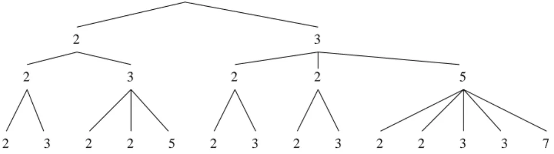
Example 5. Prime numbers and rational generating functions
Amazingly, it is possible to construct a generating tree whose set of labels is the set of prime numbers but that has a rational generating function F(z). This is a bit unexpected, as prime numbers are usually thought “too irregular” to be associated with rational generating functions. For n ≥ 1, let pn denote the nth prime; hence (p1, p2, p3, . . .) = (2,3,5, . . .).
Assume for the moment that the Goldbach conjecture is true: every even number larger than 3 is the sum of two primes. Remember that, according to Bertrand’s postulate, pn+1 <2pn
for all n(see, e.g., [23, p. 140]).
For n ≥1, the number 2pn−pn+1+ 3 is an even number larger than 3. Let qn and rn
be two primes such that 2pn−pn+1+ 3 = qn+rn. In particular, q1 =r1 = 2. Consider the
system
[(2),{(pn);(pn+1)(qn)(rn)(2)pn−3}].
It satisfies the criterion of Proposition 2, with σ(k) = 4k−3. Hence, the generating function of the associated generating tree is
F(z) = 1−2z 1−4z+ 3z2 = 1 2 1 1−z + 1 1−3z .
Consequently, the number of nodes at levelnis simplyfn= (1 + 3n)/2. This can be checked
on the first few levels of the tree drawn in Figure 2.
Now, one can object that the Goldbach conjecture is not proved; however, it is known that every even number is the sum of at most six primes [22], and a similar example can be constructed using this result.
2 2 3 3 7 2 3 2 2 5 2 3 2 3 2 2 3 2 2 3 2 5
Figure 2: A generating tree with prime labels and rational generating function.
Proposition 2 can be adapted to apply to systems that “almost” satisfy the criterion of Proposition 2, like System (2.c) or (2.d). Let us consider a system of the form
(s0), (k);e[0]1 (k), . . . , e[0]k (k) ifk is even,
(k);e[1]1 (k), . . . , e[1]k (k) ifk is odd.
Assume, moreover, that:
(i) the corresponding functionsσ0 and σ1 are affine and have the same leading coefficient
α, sayσ0(k) =αk+β0 andσ1(k) =αk+β1;
(ii) exactly m odd labels occur in the right-hand side of each rule, for somem≥0.
Proposition 3 If a system satisfies properties (i) and (ii) above, then
F(z) = 1 + (s0−α)z+ (s1−αs0−β0)z
2
1−αz−β0z2−m(β1−β0)z3 .
Of course, if β0 =β1, we recover the generating function of Proposition 2.
Proof. The proof is similar to that of Proposition 2. The only new ingredient is the fact
that, forn≥1, the number of nodes of odd label at level nismfn−1.
System (2.c) satisfies properties (i) and (ii) above with α = 3, β0 = −1, β1 = 0, m= 1,
s0 = 2 ands1 = 5. Consequently, its generating function isF(z) = 1−3z1+−zz2
−z3. System (2.d), although very close to (2.c), does not satisfy property (ii) above, so that Proposition 3 does not apply. However, another minor variation on the argument of Proposition 2, based on the fact that the number on of odd labels at level n satisfies on = 2(fn−1−on−1), proves the
rationality of F(z).
Alternatively, rationality follows from the last criterion of this section, which is of a different nature. We consider systems [(s0),{(k) ; (e1(k))(e2(k)). . .(ek(k))}] that can be
written as
[(s0),{(k) ;(c1(k))(c2(k)). . .(ck−m(k))(k+a1)(k+a2). . .(k+am)}] (4)
where 1 ≤ a1 ≤ a2 ≤ · · · ≤ am and the functions ci are uniformly bounded. Let C =
Proposition 4 Consider the system (4), and let πj,k =|{i≤j:ei(j) =k}|. If all the series
X
j≥1 πj,k tj
for k≤C are rational, then so is the series F(z).
Proof. We form an infinite system of equations defining the series Fk(z) by writing Eq. (2)
for allk≥1. In particular, for k > C, we obtain
Fk(z) =z m
X
ℓ=1
Fk−aℓ(z),
with Fj(z) = 0 if j ≤ 0. This part of the system is easy to solve in terms of F1, . . . , FC.
Indeed, fork∈Z: Fk(z) = C X i=1 Pi,k(z)Fi(z) (5)
where thePi,k are polynomials in z defined by the following recurrence: for alli≤C,
Pi,k(z) = 0 ifk≤0, [k=i] if 0< k≤C, z m X ℓ=1 Pi,k−aℓ(z) if k > C. (6) Using (5), we find F(z) =X k≥1 Fk(z) = C X i=1 Fi(z) X k≥1 Pi,k(z) .
According to (6), for alli≤C, the series Pk≥1Pi,k(z)tk is a rational function of z and t, of
denominator 1−zPℓtaℓ. Att= 1, it is rational inz. Hence, to prove the rationality of F(z), it suffices to prove the rationality of theFi(z), fori≤C.
Let us go back to theC first equations of our system; using (5), we find, for k≤C:
Fk(z) = [k=s0] +z C X i=1 Fi(z) X j≥1 Pi,j(z)πj,k .
Again, Pj≥1Pi,j(z)πj,ktj is a rational function of z and t (the Hadamard product of two
rational series is rational). Thus the series Fk(z), for k ≤ C, satisfy a linear system with
rational coefficients: they are rational themselves, as well asF(z).
Examples (2.a), (2.c), (2.d) and (2.e) have the form (4). The above proposition implies that the first three have a rational generating function. System (2.e) will be discussed in Section 4, and proved to have a transcendental generating function.
3
Factorial walks and algebraic systems
In this section, we consider systems that are of afactorial form. By this, we mean informally that the set of successors of (k) is a finite modification of the integer interval {1,2, . . . , k}. As was detailed in the introduction, ECO-systems can be rephrased in terms of walks over the integer half-line. We thus consider the problem of enumerating walks over the integer half-line such that the set of allowed moves from point k is a finite modification of the integer interval [0, k]. We shall mostly study modifications around the point k (although some examples where the interval is modified around 0 as well are given at the end of the section). Precisely, a factorial walk is defined by a finite (multi)set A ⊂Z and a finite set
B ⊂N+, where N+ ={1,2,3, . . .}, specifying respectively the allowed supplementary jumps (possibly labeled) and theforbidden backward jumps. In other words, the possible moves from
k are given by the rule:
(k);[0, k−1]\(k−B) ∪ (k+A). (7) Observe that these walk models are not necessarily ECO-systems, first because we allow labels to be zero – but a simple translation can take us back to a model with positive labels – and second because we do not require (k) to have exactly k successors.
We say that an ECO-system is factorial if a shift of indices transforms it into a factorial walk. Hence the rules of a factorial ECO-system are of the form
(k+r);[r, k+r−1]\(k+r−B) ∪ (k+r+A),
that is,
(k);[r, k−1]\(k−B) ∪ (k+A) fork≥r ≥1. (8) The generating function F(z) for such an ECO-system, taken with axiom (s0), equals the
generating function for the walk model (7), taken with axiom (s0−r). However, remember
that the rewriting rules defining a generating tree have to obey the additional condition that a node labeled k has exactly k successors. Taking k = r in (8), this implies that r = |A|. Taking k > r+ maxB, this implies thatr+|B|=|A|, so that finally B =∅. Hence, strictly speaking, either one has a “fake” factorial ECO-system (that is some of its initial rules are not of the factorial type), either one has a “real” factorial ECO-system and then it is given by rules of the form
(k);[r, k−1] ∪ (k+A) fork≥r ≥1,
where A is a multiset of integers of cardinality r. For instance, Systems (2.f) and (2.g) are factorial. We shall prove that all factorial walks have an algebraic generating function. The result naturally applies to factorial ECO-systems.
We consider again the generating function F(z, u) = Pn,k≥0fn,kznuk, where fn,k is the
number of walks of length n ending at point k. We also denote by Fk(z) the coefficient of
uk in this series, and by f
n(u) the coefficient of zn. The first ingredient of the proof is a
linear operator M, acting on formal power series inu, that encodes the possible moves. More precisely, for all n≥0, we will have:
M[fn](u) =fn+1(u).
— The set of moves fromkto all the positions 0,1, . . . , k−1 is described by the operator
L0 that mapsuk to u0+u1+· · ·+uk−1= (1−uk)/(1−u). AsL0 is a linear operator,
we have, for any series g(u):
L0[g](u) =
g(1)−g(u) 1−u .
— The fact that transitions near k are modified, with those of type k+α (with α ∈A) allowed and those of type k−β (with β ∈ B) forbidden, is expressed by a Laurent polynomial P(u) = a X k=−b pkuk=A(u)−B(u) with A(u) = X α∈A uα and B(u) = X β∈B u−β.
The degree of P is a := maxA, the largest forward jump and b := max(0,−B,−A) is largest forbidden backward jump or the largest supplementary backward jumps (we take b= 0 if the setB is empty).
The operator
L[g](u) :=L0[g](u) +P(u)g(u) describes the extension of a walk by one step.
— Finally, the operator M is given by
M[g](u) =L[g](u)− {u<0}L[g](u),
where {u<0}h(u) is the sum of all the monomials in h(u) having a negative exponent. Hence M is nothing but L stripped of the negative exponent monomials, which corre-spond to walks ending on the nonpositive half-line. Observe that, for any series g(u), the only part of L[g](u) that is likely to contain monomials with negative exponents is
P(u)g(u). Consequently, M[g](u) =L[g](u)− {u<0}[P(u)g(u)] and if g(u) =Pkgkuk, then {u<0}[P(u)g(u)] = b X i=1 i−1 X k=0 gkp−iuk−i = b−1 X k=0 gkrk(u). (9)
Assume for simplicity that the initial point of the walk is 0; other cases follow the same argument. The linear relation fn+1(u) =M[fn](u), together withf0(u) = 1, yields
F(z, u) = 1 +zM[F](z, u) = 1 +z F(z,1) −F(z, u) 1−u +P(u)F(z, u) +{u <0}[P(u)F(z, u)].
Thanks to (9), we can write
{u<0}[P(u)F(z, u)] =
b−1
X
k=0
where rk(u) is a Laurent polynomials (defined by Equation 9) whose exponents belong to
[k−b,−1]. Thus, F(z, u) satisfies the following functional equation:
F(z, u) 1 + z 1−u −zP(u) = 1 +zF(z,1) 1−u +z b−1 X k=0 rk(u)Fk(z). (10)
Let us take an example. The moves
(k);(0)(1)· · ·(k−5)(k−3)(k−1)(k)(k+ 7)(k+ 9),
lead toA(u) =u0+u7+u9 and B(u) =u−4+u−2. Moreover,
{u<0}[B(u)F(z, u)] = (u−2+u−4)F0(z) + (u−1+u−3)F1(z) +u−2F2(z) +u−1F3(z),
so that the functional equation defining F(z, u) is
F(z, u) 1 + z 1−u −z(1 +u 7+u9−u−4−u−2)= 1 + zF(z,1) 1−u +z(u −2+u−4)F 0(z) +z(u−1+u−3)F1(z) +zu−2F2(z) +zu−1F3(z).
The second ingredient of the proof, sometimes called the kernel method, seems to belong to the “mathematical folklore” since the 1970’s. It has been used in various combinatorial problems [10, 18, 20] and in probabilities [14]. See also [8, 9, 21] for more recent and system-atic applications. This method consists in cancelling the left-hand side of the fundamental functional equation (10) by couplingzandu, so that the coefficient of the (unknown) quantity
F(z, u) is zero. This constraint definesu as one of the branches of an algebraic function ofz. Each branch that can be substituted analytically into the functional equation yields a linear relation between the unknown seriesF(z,1) andFk(z), 0≤k < b. If enough branches can be
substituted analytically, we obtain a system of linear equations, whose solution gives F(z,1) and theFk(z) as algebraic functions. From there, an expression forF(z, u) also results in the
form of a bivariate algebraic function.
Let us multiply Eq. (10) by ub(1−u) to obtain an equation with polynomial coefficients
(remind that we take b = 0 if the set B of forbidden backward steps is empty). The new equation reads K(z, u)F(z, u) =R(z, u), whereK(z, u) is the kernel of the equation:
K(z, u) = ub(1−u) 1 + z 1−u −zP(u) , = ub(1−u) +zub−z(1−u)X α∈A uα+b+z(1−u)X β∈B ub−β. (11) This polynomial has degree a+b+ 1 in u, and hence, admitsa+b+ 1 solutions, which are algebraic functions of z. The classical theory of algebraic functions and the Newton polygon construction enable us to expand the solutions near any point as Puiseux series (that is, series involving fractional exponents; see [11]). Thea+b+ 1 solutions, expanded around 0, can be classified as follows:
— b “small” branches, denoted by u1, . . . , ub, are power series in z1/b whose first nonzero
term is ζz1/b, withζb+ 1 = 0;
— a“large” branches, denoted byv1, . . . , va, are Laurent series inz1/a whose first nonzero
term is ζz−1/a, withζa+ 1 = 0.
In particular, all the roots are distinct. (It is not difficult to check “by hand” the existence of these solutions: for instance, plugging z = tb and u =tw(t) in K(z, u) = 0 confirms the
existence of the bsmall branches.) Note that there are exactly b+ 1 finite branches: the unit branch u0 and the b small branches u1, . . . , ub. As F(z, u) is a series in z with polynomial
coefficients in u, these b+ 1 series ui, having no negative exponents, can be substituted for
u in F(z, u). More specifically, let us replace u by ui in (10): the right-hand side of the
equation vanishes, giving a linear equation relating the b+ 1 unknown series F(z,1) and
Fk(z), 0≤k < b. Hence theb+ 1 finite branches give a set ofb+ 1 linear equations relating
theb+ 1 unknown series. One could solve directly this system, but the following argument is more elegant.
The right-hand side of (10), once multiplied byub(1−u), is
R(z, u) =ub(1−u) 1 + z 1−uF(z,1) +z b−1 X k=0 rk(u)Fk(z) ! .
By construction, it is a polynomial inu of degree b+ 1 and leading coefficient −1. Hence, it admits b+ 1 roots, which depend on z. Replacing u by the series u0, u1, . . . , ub in Eq. (10)
shows that these series are exactly theb+ 1 roots ofR, so that
R(z, u) =−
b
Y
i=0
(u−ui).
Let pa := [ua]P(u) be the multiplicity of the largest forward jump. Then the coefficient of
ua+b+1 inK(z, u) isp
az, and we can write
K(z, u) =paz b Y i=0 (u−ui) a Y i=1 (u−vi). Finally, as K(z, u)F(z, u) =R(z, u), we obtain F(z, u) = − Qb i=0(u−ui) ub(1−u) +zub−zub(1−u)P(u) =− 1 pazQai=1(u−vi) . (12) We have thus proved the following result.
Proposition 5 The generating functionF(z, u)for factorial walks defined by(7)and starting
from 0 is algebraic; it is given by(12), where u0, . . . , ub (resp. v1, . . . , va) are the finite (resp.
infinite) solutions at z = 0 of the equation K(z, u) = 0 and the kernel K is defined by (11). In particular, the generating function for all walks, irrespective of their endpoint, is
F(z,1) =−1 z b Y i=0 (1−ui),
and the generating function forexcursions, i.e., walks ending at 0, is, for b <0: F(z,0) = (−1) b z b Y i=0 ui,
(forb= 0, the relation becomes F(z,0) = 1+(−z−p1)b0zQbi=0ui.)
These results could be derived by a detour via multivariate linear recurrences, and the present treatment is closely related to [9, 21]; however, our results were obtained independently in March 1998 [1].
The asymptotic behaviour of the number ofn-step walks can be established via singularity analysis or saddle point methods. The series ui have “in general” a square root singularity,
yielding an asymptotic behaviour of the formAµnn−3/2.We plan to develop this study in a
forthcoming paper.
Example 6. Catalan numbers
This is the simplest factorial walk, (k) ; (0)(1). . .(k)(k + 1), which corresponds to the ECO-system (2.f). The operator M is given by
M[f](u) = f(1)−f(u)
1−u + (1 +u)f(u).
The kernel is K(z, u) = 1−u+z−z(1−u)(1 +u) = 1−u+zu2, henceu0(z) = 1−
√ 1−4z 2z , so that F(z,1) =−1−u0 z = 1−2z−√1−4z 2z2 = X n≥1 2n n ! zn−1 n+ 1,
the generating function of the Catalan numbers (sequence M14591). This result could be expected, given the obvious relation between these walks and Lukasiewicz codes. 2
Example 7. Motzkin numbers
This example, due to Pinzani and his co-authors, is derived from the previous one by forbid-ding “forward” jumps of length zero. The rule is then
(k);(0)· · ·(k−1)(k+ 1).
The operator M is
M[f](u) = f(1)−f(u)
1−u +uf(u).
The kernel is K(z, u) = 1−u+z−zu(1−u) = 1 +z−u(1 +z) +zu2, leading to
F(z,1) = 1−z− √
1−2z−3z2
2z2 = 1 +z+ 2z
2+ 4z3+ 9z4+ 21z5+O(z6),
the generating function for Motzkin numbers (sequenceM1184). 2
1
Example 8. Schr¨oder numbers
This example is also due to the Florentine group. The rule is (k);(0). . .(k−1)(k)(k+ 1)2. From Proposition 5, we derive
F(z,1) = 1−3z− √
1−6z+z2
4z2 = 1 + 3z+ 11z
2+ 45z3+ 197z4+O(z5).
The coefficients are the Schr¨oder numbers (M2898: Schr¨oder’s second problem). We give in Table 1 at the end of the paper a generalization of Catalan and Schr¨oder numbers, corre-sponding to the rule (k);(0). . .(k−1)(k)(k+ 1)m. This generalized rule has recently been shown to describe a set of permutations avoiding certain patterns [19]. 2 The above examples were all quadratic. However, it is clear from our treatment that algebraic functions of arbitrary degree can be obtained: it suffices that the set of “exceptions” around k have a span greater than 1. Let us start with a family of ECO-systems where supplementary forward jumps of length larger than one are allowed.
Example 9. Ternary trees, dissections of a polygon, and m-ary trees The ECO-system with axiom (s0) = (3) and rule
(k);(3)(4)· · ·(k)(k+ 1)(k+ 2) is equivalent to the walk
(k);(0)(1)· · ·(k)(k+ 1)(k+ 2).
The kernel is K(z, u) = 1−u+zu3, and the generating function
F(z,1) = X n≥1 3n n ! zn−1 2n+ 1 counts ternary trees (M2926).
More generally, the system with axiom (m) and rewriting rules (k);(m)· · ·(k)(k+ 1)(k+ 2)· · ·(k+m−1)
yields the m-Catalan numbers, mnn/((m−1)n+ 1), that count m-ary trees. The kernel is 1−u+zum and the generating function F(z,1) satisfies F(z,1) = (1 +zF(z,1))m. In
particular, the 4-Catalan numbers 4nn/(3n+ 1) appear in [24] (sequenceM3587) and count dissections of a polygon.
2 In the above examples, all backward jumps are allowed. In other words, each of these examples corresponds to an ECO-system. Let us now give an example where backward jumps of length 1 are forbidden.
Example 10.
Consider the following modification of the Motzkin rule: (k);(0)· · ·(k−2)(k+ 1).
The kernel is now K(z, u) = u(1−u) +zu−z(1−u)(u2 −1), and, according to (12), the series F(z) =F(z,1) is given by F(z) = 1/[z(v1 −1)], wherev1 satisfiesK(z, v1) = 0 and is
infinite atz= 0. Denoting G=zF(z), we find that the algebraic equation definingGis:
G=z 1 + 2G+G 2+G3
1 +G .
2 So far, we have only dealt with walks for which the set of allowed moves was obtained by modifying the interval [0, k] aroundk. One can also modify this interval around 0: we shall see – in examples – that the generating function remains algebraic. However, it is interesting to note that in these examples, the kernel method does not immediately provide enough equations between the “unknown functions” to solve the functional equation.
Let us first explain how we modify the interval [0, k] around 0. The walks we wish to count are still specified by a multiset A of allowed supplementary jumps and a set B of forbidden backward jumps. But, in addition, we forbid backward jumps to end up inC, where C is a given finite subset of N. In other words, the possible moves fromk are given by the rule
(k);[0, k−1]\(C∪(k−B)) ∪ (k+A).
Again, we can write a functional equation defining F(z, u):
F(z, u) = 1 +z F(z,1)−F(z, u) 1−u +P(u)F(z, u) + b−1 X k=0 rk(u)Fk(z)− X γ∈C uγGγ(z) , (13) where, as above, P(u) = X α∈A uα− X β∈B u−β and rk(u) = X β>k, β∈B uk−β,
the new terms in the equations being
Gγ(z) =F(z,1)− γ X k=0 Fk(z)− X β∈B Fβ+γ(z).
Observe that the first three terms are the same as in the case C = ∅. The equation, once multiplied by ub(1−u), reads K(z, u)F(z, u) =R(z, u) where K(z, u) is given by (11) and
R(z, u) =ub(1−u) 1 +zF(z,1) 1−u +z b−1 X k=0 rk(u)Fk(z)−z X γ∈C uγGγ(z) .
The kernel is not modified by the introduction ofC. As above, it has degreea+b+1 inu, and admits b+ 1 finite roots u0, . . . , ub aroundz = 0. However, R(z, u) now involves b+ 1 +|C|
unknown functions, namelyF(z,1), theFk(z), 0≤k < band theGγ(z), γ ∈C. The degree
of R in u is no longer b+ 1 but b+c+ 1, where c = maxC. The b+ 1 roots of K that can be substituted for u in Eq. (13) provide b+ 1 linear equations between the b+|C|+ 1 unknown functions. Additional equations will be obtained by extracting the coefficient ofuj
from Eq. (13), for some values of j. In general, we have:
Fj(z) = [j= 0] +z X α∈A Fj−α(z) +z[j6∈C] F(z,1)− j X k=0 Fk(z)− X β∈B Fj+β(z) . (14)
It is possible to construct a finite subset S ⊂ N such that the combination of the b+ 1 equations obtained via the kernel method and the equations (14) written forj∈S determines all unknown functions as algebraic functions of z – more precisely, as rational functions of z
and the rootsu0, . . . , ub of the kernel. However, this is a long development, and these classes
of walks play a marginal role in the context of ECO-systems. For these reasons, we shall merely give two examples. The details on the general procedure for constructing the set S
can be found in [7]. Example 11.
This example is obtained by modifying the Motzkin rule of Example 7 around the point 0. Take A=C ={1} and B=∅. The rewriting rule is
(k);(0)(2)(3)· · ·(k−1)(k+ 1).
The functional equation reads
(1−u+z−zu(1−u))F(z, u) = 1−u+zF(z,1)−zu(1−u)G1(z), (15)
with G1(z) =F(z,1)−F0(z)−F1(z). The kernel has aunique finite root at z= 0:
u0 =
1 +z−√1−2z−3z2
2z ,
whereas the right-hand side of Eq. (15) contains two unknown functions. Writing Eq. (14) for j= 0 and j= 1 yields
F0(z) = 1 +z(F(z,1)−F0(z)) and F1(z) =zF0(z).
These two equations allow us to expressF0 and F1, and henceG1, in terms of F(z,1): G1(z) = (1−z)F(z,1)−1.
This equation relates the two unknown functions of Eq. (15). We replace G1(z) by the above
expression in (15), so that only one unknown function, namely F(z,1), is left. The kernel method finally gives:
F(z,1) = 3−3z 2−2z3−(1 +z)√1−2z−3z2 2(1−z−z2+z3+z4) = 1 +z+ 2z 2+ 3z3+ 6z4+ 12z5+O(z6). 2 Example 12.
Let us choose A={1},B ={2}et C={2}. The rewriting rule is now: (k)→(0)(1)(3)(4)(5). . .(k−3)(k−1)(k+ 1).
The functional equation reads h
=u2(1−u) +zu2F(z,1) +z(1−u) [F0(z) +uF1(z)]−zu4(1−u)G2(z), (16)
with G2(z) = F(z,1)−F0(z)−F1(z)−F2(z)−F4(z). Only three roots, u0, u1, u2 can be
substituted foruin the kernel, while the right-hand side of the equation contains four unknown functions,F(z,1), F0(z), F1(z) and G2(z). Writing (14) for j= 0,1 and 2 yields
F0(z) = 1 +z[F(z,1)−F0(z)−F2(z)],
F1(z) =zF0(z) +z[F(z,1)−F0(z)−F1(z)−F3(z)], F2(z) =zF1(z).
The second equation is not of much use but, by combining the first and third one, we find
F0(z) =
1 +z[F(z,1)−zF1(z)]
1 +z .
Replacing F0(z) by this expression in (16) gives:
h u2(1−u) +zu2−zu3(1−u) +z(1−u)iF(z, u) =u2(1−u)+z(1−u) 1 +z +zF(z,1) u2+ z(1−u) 1 +z +z(1−u)F1(z) " u− z 2 1 +z # −zu4(1−u)G2(z). (17)
We are left with three unknown functions, related by three linear equations obtained by cancelling the kernel. Solving these equations would give F(z,1) as an enormous rational function of z, u0, u1 and u2, symmetric in the ui. This implies that F(z,1) can also be
written as a rational function of z and v ≡ v1, the fourth and last root of the kernel. In
particular, F(z,1) is algebraic of degree at most 4.
In order to obtain directly an expression of F(z,1) in terms of z and v, we can proceed as follows. LetR′(z, u) denote the right-hand side of Eq. (17). Then R′(z, u) is a polynomial
inu of degree 5, and three of its roots are u0, u1, u2. Consequently, as a polynomial inu, the
kernel K(z, u) divides (u−v)R′(z, u).
Let us evaluate (u−v)R′(z, u) modulo K(z, u): we obtain a polynomial of degree 3 in
u, whose coefficients depend on z, v, F(z,1), F1(z) and G2(z). This polynomial has to be
zero: this gives a system of four (dependent) equations relating the three unknown functions
F(z,1), F1(z) and G2(z). Solving the first three of these equations yields
F(z,1) = 1 +z+z
2−(z+ 1)zv+ (z+ 1)zv2−z2v3
1−z2−z(1−z2)v+z3v3
= 1 +z+ 2z2+ 3z3+ 6z4+ 11z5+ 23z6+ 47z7+ 101x8+O(z9).
Eliminating v between this expression and K(z, v) = 0 gives a quartic equation satisfied by
F(z,1). 2
4
Transcendental systems
4.1 Transcendence
The radius of convergence of an algebraic series is always positive. Hence, one possible reason for a system to give a transcendental series is the fact that its coefficients grow too fast, so
that its radius of convergence is zero. This is the case for System (2.h), as proved by the following proposition.
Proposition 6 Let b be a nonnegative integer. For k≥1, let m(k) =|{i: ei(k)≥k−b}|.
Assume that:
1.for all k, there exists a forward jump from k (i.e., ei(k)> k for some i),
2.the sequence (m(k))k is nondecreasing and tends to infinity.
Then the (ordinary) generating function of the system has radius of convergence 0.
Proof. Lets0 be the axiom of the system. Let us denote byhn the productm(s0+b)m(s0+
2b)· · ·m(s0+nb). Let us prove that the generating tree contains at least hn nodes at level
n(b+ 1). At level nb, take a nodevlabeled k, withk≥s0+nb. Such a node exists thanks to
the first assumption. By definition of m(k), this nodev hasm(k) sons whose label is at least
k−b. Asm is non decreasing,v has at least m(s0+nb) sons of label at least s0+ (n−1)b.
Iterating this procedure shows that, at levelnb+i, at leastm(s0+ (n−i+ 1)b)· · ·m(s0+nb)
descendants ofvhave a label larger than or equal tos0+ (n−i)b, for 0< i≤n. In particular,
for i=n, we obtain at level n(b+ 1) at least hn descendants ofv whose label is at least s0.
Hence fn(b+1) ≥ hn. But as hn/hn−1 = m(s0 +nb) goes to infinity with n, the series
P
nhnzn(b+1) has radius of convergence 0, and the same is true for F(z) =Pnfnzn.
In particular, this proposition implies thatthe generating function of any ECO-system in which the length of backward jumps is bounded has radius of convergence 0. Many examples of this type will be given in the next subsection, in which we shall study whether the corre-sponding generating function is holonomic or not. The following example, in which backward jumps are not bounded, was suggested by Nantel Bergeron.
Example 13. A fake factorial walk
Consider the system with axiom (1) and rewriting rules{(k);(2)(4)· · ·(2k)}. Proposition 6 applies with b = 0 and m(k) = 1 +⌊k/2⌋. Note that the radius of convergence of F(z) is zero although all the functionsei are bounded, and indeed constant: ei(k) = 2ifor all k≥i.
The seriesF(z) is of course transcendental. Note, however, thatF(z, u) satisfies a functional equation that is at first sight reminiscent of the equations studied in Section 3:
F(z, u) =u+zu2 F(z,1)−F(z, u 2)
1−u2 .
2 The following example shows that Proposition 6 is not far from optimal: an ECO-system in which all functionsei grow linearly can have a finite radius of convergence.
Example 14.
The system with axiom (1) and rules (k);(⌈k/2⌉)k−1(k+ 1) leads to a generating function
with a positive radius of convergence.
Let us start from the recursion defining the numbersfn,k. We have f0,1= 1 and for n≥1, fn+1,k=fn,k−1+ (2k−1)fn,2k+ (2k−2)fn,2k−1.
n k 1 2 3 4 5 6 0 1 1 0 1 2 1 0 1 3 0 3 0 1 4 3 3 3 0 1 5 3 9 7 3 0 1 n k 0 1 2 3 4 5 0 1 1 1 0 2 1 0 1 3 1 0 3 0 4 1 0 3 3 3 5 1 0 3 7 9 3
Table 1: The numbers fn,k andgn,k. Observe the convergence of the coefficients.
The largest label occurring at level n in the tree is n+ 1. Let us introduce the numbers
gn,k =fn,n−k+1, fork≤n. The above recursion can be rewritten as:
gn+1,k =gn,k+ (2n−2k+ 3)gn,2k−n−3+ (2n−2k+ 2)gn,2k−n−2. (18)
We have gn,k = 0 for k < 0. Hence Eq. (18) implies that for k ≥ 0, the sequence (gn,k)n is
nondecreasing and reaches a constant value g(k) as soon asn≥2k−1 (see Table 1). Going back to the numberfn of nodes at level n, we have
fn= n X k=0 gn,k≤ n X k=0 g(k). But X n≥0 zn n X k=0 g(k) = 1 1−z n X k=0 g(k)zk,
and hence it suffices to prove that the generating function for the numbersg(k) has a finite radius of convergence, that is, that these numbers grow at most exponentially.
Writing (18) for n+ 1 = 2k−i, for 1≤i≤k, we obtain:
g2k−i,k=g2k−i−1,k+ (2k−2i+ 1)g2k−i−1,i−2+ (2k−2i)g2k−i−1,i−1.
Iterating this formula foribetween 1 and kyields
g(k) = g2k−1,k = k X i=1 [(2k−2i+ 1)g2k−i−1,i−2+ (2k−2i)g2k−i−1,i−1] ≤ k X i=1 [(2k−2i+ 1)g(i−2) + (2k−2i)g(i−1)] = k−X2 i=0 (4k−4i−5)g(i).
This inequality, together with the fact that g(0) = 1, implies that for all k≥0,g(k) ≤ge(k), where the sequence ge(k) is defined by eg(0) = 1 and eg(k) =Pk−i=02(4k−4i−5)eg(i) for k >0. But the series Pkge(k)zk is rational, equal to (1−z)2/(1−2z−2z2−z3), and has a finite radius of convergence. Consequently, the numbersge(k) andg(k) grow at most exponentially. 2
Algebraic generating functions are strongly constrained in their algebraic structure (by a polynomial equation) as well as in their analytic structure (in terms of singularities and asymptotic behaviour). In particular, they have a finite number of singularities, which are
algebraic numbers, and they admit local asymptotic expansions that involve only rational exponents. A contrario, a generating function that has infinitely many singularities (e.g., a natural boundary) or that involves a transcendental element (e.g., a logarithm) in a local asymptotic expansion is by necessity transcendental; see [16] for a discussion of such tran-scendence criteria. In the case of generating trees, this means that the presence of a condition involving a transcendental element is expected to lead to a transcendental generating function. This is the case in the following example.
Example 15. A Fredholm system
We examine System (2.e), in which the rules are irregular at powers of 2: (s0) = (2), (k);(2)k−2(3−[∃p:k= 2p])(k+ 1), k≥2.
This example will involve the Fredholm seriesh(z) :=Pp≥1z2p, which is well-known to admit the unit circle as a natural boundary. (This can be seen by way of the functional equation
h(z) =z2+h(z2), from which there results thath(z) is infinite at all iterated square-roots of
unity.) According to Eq. (2), we have, for k >3,Fk(z) =zFk−1(z),so that Fk(z) =zk−3F3(z) fork≥3.
Now, writing Eq. (2) fork= 2 gives
F2(z) = 1 +z X k≥3 (k−2)Fk(z) +z X p≥1 F2p(z) = 1 + z (1−z)2F3(z) +zF2(z) +F3(z) h(z) z2 −1 = 1 +zF2(z) +F3(z) z (1−z)2 + h(z) z2 −1 . For k= 3, we obtain: F3(z) = zF2(z) +z X k≥3, k6=2p Fk(z) = zF2(z) +F3(z) 1 1−z − h(z) z2 .
Solving for F2(z) andF3(z), then summing (F(z) =F2(z) +F3(z)/(1−z)), we obtain:
F(z) = (1−z)
2h(z)
(1−2z)(1−z)2h(z)−z4 = 1 + 2z+ 5z
2+ 14z3+ 39z4+ 108z5+O(x6).
The functions h(z) andF(z) are rationally related, so thatF(z) is itself transcendental. The series h has radius 1, but the denominator ofF vanishes beforez reaches 1 – actually, before
z reaches 1/2. Hence the radius of F is the smallest root of its denominator. Its value is
4.2 Holonomy
In the transcendental case, one can also discuss the holonomic character of the generating function F(z).
A series is said to beholonomic, or D-finite[25], if it satisfies a linear differential equation with polynomial coefficients in z. Equivalently, its coefficients fn satisfy a linear recurrence
relation with polynomial coefficients in n. Consequently, given a sequence fn, the ordinary
generating function Pnfnzn is holonomic if and only if the exponential generating function
P
nfnzn/n! is holonomic. The set of holonomic series has nice closure properties: the sum or
product of two of them is still holonomic, and the substitution of an algebraic series into an holonomic one gives an holonomic series. Holonomic series include algebraic series, and have a finite number of singularities. This implies that Example 15, for which F(z) has a natural boundary, is not holonomic.
We study below five ECO-systems that, at first sight, do not look to be very different. In particular, for each of them, forward and backward jumps are bounded. Consequently, Proposition 6 implies that the corresponding ordinary generating function has radius of con-vergence zero. However, we shall see that the first three systems have an holonomic generating function, while the last two have not. We have no general criterion that would allow us to distinguish between systems leading to holonomic generating functions and those leading to nonholonomic generating functions.
Among the systems with bounded jumps, those for whichei(k)−k belongs to {−1,0,1}
for all i≤k have a nice property: the generating function for the corresponding excursions (walks starting and ending at level 0) can be written as the following continued fraction [15]:
1 1−b0z− a1c0z2 1−b1z− a2c1z 2 1−b2z− a3c2z2 · · · ,
where the coefficients ak, bk and ck are the multiplicities appearing in the rules, which read
(k);(k−1)ak(k)bk(k+ 1)ck. Example 16. Arrangements
The system (k);(k)(k+ 1)k−1 with axiom (s0) = (2) generates a sequence that starts with 1,2,5,16,65,326 (M1497). It is not hard to see that the triangular array fn,k+2 is given by
the arrangement numbers k! nk, so that the exponential generating function (EGF) of the sequence is e F(z, u) = X n≥0,k≥2 fn,kuk zn n! = u2ez 1−uz.
This system satisfies the conditions of Proposition 6 withb= 0 andm(k) =k. Accordingly, one hasfn∼e n!, so that theordinary generating functionF(z) has radius of convergence 0
and cannot be algebraic. However,Fe(z,1) =ez/(1−z) is holonomic, and so is F(z).
2
Example 17. Involutions and Hermite polynomials The system (k) ;(k−1)k−1(k+ 1) with axiom (s
with 1,1,2,4,10,26,76 (M1221). These numbers count involutions: more precisely, one easily derives from the recursion satisfied by the coefficients fn,k that fn,k is the number of
involutions on n points, k−1 of which are fixed. Proposition 6 applies with b = 1 and
m(k) =k.
The corresponding EGF is e F(z, u) = X n≥0,k≥1 fn,kuk zn n! =uexp zu+ z2 2 ! , (19)
and its value at u= 1 is holonomic.
The polynomials fn(u) = Pkfn,kuk counting involutions on n points are in fact closely
related to the Hermite polynomials, defined by: X n≥0 Hn(x) tn n! = exp xt− t2 2 ! .
Indeed, comparing the above identity with (19) shows thatfn(u) =u inHn(−iu). 2
Example 18. Partial permutations and Laguerre polynomials
The rewriting rule (k);(k+ 1)k−1(k+ 2), taken with axiom (2), generates a sequence that
starts with 1,2,7,34,209, ... (M1795). From the recursion satisfied by the coefficients fn,k,
we derive that fn,n+k is the number of partial injections of {1,2, . . . , n} into itself in which
k−2 points are unmatched. From this, we obtain: e F(z, u) = u 2 1−uzexp u2z 1−uz ! =u2X n≥0 Ln(−u) (uz)n n!
whereLn(u) is the nth Laguerre polynomial. Again,Fe(z,1) is holonomic. 2
The next two systems, as announced, lead to nonholonomic generating functions. Example 19. Set partitions and Stirling polynomials
Let us consider the system [(1),(k) ; (k)k−1(k+ 1)]. From the recursion satisfied by the coefficientsfn,k, we derive thatfn,k+1is equal to the Stirling number of the second kindnk ,
which counts partitions ofnobjects into knonempty subsets. The corresponding EGF is e
F(z, u) =uexp (u(expz−1)).
Atu= 1, this generating function specializes to e F(z,1) = exp(exp(z)−1)) = X n≥0 Bn zn n! = 1 +z+ 2 z2 2! + 5 z3 3! + 15 z4 4! + 52 z5 5! + 203 z6 6! +. . . This is the exponential generating function of the Bell numbers (M1484). It is known that logBn=nlogn−nlog logn+O(n) (see [20]), and this cannot be the asymptotic behaviour of
the logarithm of the coefficients of an holonomic series (see [29] for admissible types). Hence, e
Example 20. Bessel numbers
We study the system with axiom (2) and rewriting rules
(2);(2)(3), (k);(k−1)(k)k−2(k+ 1), k≥3. (20) We shift the labels by 2 to obtain a walk model with axiom (0) and rules
(0);(0)(1), (k);(k−1)(k)k(k+ 1), k≥1.
The corresponding bivariate generating function F(z, u) satisfies the functional differential equation
F(z, u)1−z(u+u−1)= 1 +z(1−u−1)F(z,0) +zu∂F ∂u(z, u),
which is certainly not obvious to solve. However, as observed in [15], it is easy to obtain a continued fraction expansion of the excursion generating function:
F(z,0) = 1+z+2z2+4z3+9z4+· · ·= 1 1−z− z 2 1−z− z 2 1−2z− z 2 1−3z−. .. = 1 1−z−z2B(z), where B(z) = PnB∗ nzn = 1 +z+ 2z2+ 5z3+ 14z4 + 43z5 + 143z6 +· · · is the generating
function of Bessel numbers (M1462) and counts non-overlapping partitions [17]. As F(z,0) itself, the series B(z) has radius of convergence zero. The fast increase of B∗
n entails
[zn]F(z,0) ∼Bn−∗ 2.
From [17], we know that logB∗
n =nlogn−nlog logn+O(n).Again, this prevents F(z,0)
from being holonomic.
In order to prove that F(z,1) itself is nonholonomic, we are going to prove that its coefficients fn have the same asymptotic behaviour as the coefficients of F(z,0). Clearly,
[zn]F(z,0) =fn,0≤
X
k
fn,k =fn.
To find an upper bound forfn, we compare the system (20) (denoted Σ1below) to the system
Σ2 with axiom (2) and rule (k);(k)k−1(k+ 1). This system generates a tree with counting
sequence gn. The form of the rules implies that the (unlabeled) tree associated with Σ1 is a
subtree of the tree associated with Σ2. Hencefn≤gn. Comparing Σ2 to the system studied
in the previous example shows thatgnis the Bell numberBn+1, the logarithm of which is also
known to benlogn−nlog logn+O(n) (see [20]). Hence logfn=nlogn−nlog logn+O(n),
Axiom System Name Id. Generating Function
Rational OGF OGF
(1) (k);(k)k−1((kmod 2) + 1) Ex. 3: Fibonacci M0692 1 1−z−z2 (2) (k);(2)k−1(k+ 1) Ex. 4: even Fibonacci M1439 1−z
1−3z+z2 (3) (k);(2)k−1(k+ 1) Ex. 4: odd Fibonacci M2741 1
1−3z+z2
Algebraic OGF OGF
(1) (k);(1)· · ·(k−1)(k+ 1) Ex. 7: Motzkin numbers M1184 1−z− √
1−2z−3z2 2z2
(2) (k);(2)· · ·(k)(k+ 1) Ex. 6: Catalan numbers M1459 1−2z− √
1−4z 2z2
(3) (k);(3)· · ·(k)(k+ 1)2 Ex. 8: Schr¨oder numbers M2898 1−3z− √ 1−6z+z2 4z2 (4) (k);(4)· · ·(k)(k+ 1)3 — M3556 1−4z− √ 1−8z+4z2 6z2 (m) (k);(m)· · ·(k)(k+ 1)m−1 — — 1−mz− √ 1−2mz+(m−2)2z2 2(m−1)z2
(3) (k);(3)· · ·(k+ 2) Ex. 9: Ternary trees M2926 F = (1 +zF)3 (4) (k);(4)· · ·(k+ 3) Ex. 9: Dissections of a polygon M3587 F = (1 +zF)4 (m) (k);(m)· · ·(k+m−1) Ex. 9: m-ary trees F = (1 +zF)m
Holonomic EGF transcendental OGF (1) (k);(k+ 1)k Permutations M1675 1/(1 −z) (2) (k);(k)(k+ 1)k−1 Ex. 16: Arrangements M1497 ez/(1−z) (1) (k);(k−1)k−1(k+ 1) Ex. 17: Involutions M1221 ez+12z2 (2) (k);(k+ 1)k−1(k+ 2) Ex. 18: Partial permutations M1795 ez/(1−z)/(1−z) (2) (k);(k−1)k−2(k)(k+ 1) Switchboard problem M1461 e2z+12z2 (2) (k);(k−1)k−2(k+ 1)2 Bicolored involutions M1648 e2z+z2
Nonholonomic OGF EGF
(1) (k);(k)k−1(k+ 1) Ex. 19: Bell numbers M1484 ee
z
−1 (2) (k);(k)k−2(k+ 1)2 Bicolored partitions M1662 e2(e
z
−1) (2) (k);(k−1)(k)k−2(k+ 1) Ex. 20: Bessel numbers M1462 —
Table 2: Some ECO-systems of combinatorial interest.
A small catalog of ECO-systems
To conclude, we present in Table 2 a small catalog of ECO-systems that lead to sequences of combinatorial interest. Several examples are detailed in the paper; others are due to West [27, 28] or Barcucci, Del Lungo, Pergola, Pinzani [4, 6, 5, 3], or are folklore. Each of them is an instance of application of our criteria.
Acknowledgements. We thank Elisa Pergola and Renzo Pinzani who presented us the
problem we deal with in this paper. We are also very grateful for helpful discussions with Jean-Paul Allouche.
References
[1] C. Banderier. Combinatoire analytique : application aux marches al´eatoires. M´emoire de DEA, Universit´e Paris VII, 1998.
[2] E. Barcucci, A. Del Lungo, and E. Pergola. Random generation of trees and other combinatorial objects. Theoretical Computer Science, 218(2):219–232, 1999.
[3] E. Barcucci, A. Del Lungo, E. Pergola, and R. Pinzani. A methodology for plane tree enumeration. Discrete Mathematics, 180(1-3):45–64, 1998.
[4] E. Barcucci, A. Del Lungo, E. Pergola, and R. Pinzani. ECO: a methodology for the enumeration of combinatorial objects. Journal of Difference Equations and Applications, 5:435–490, 1999.
[5] E. Barcucci, A. Del Lungo, E. Pergola, and R. Pinzani. From Motzkin to Catalan permutations. Discrete Mathematics, 217(1–3):33–49, 2000.
[6] E. Barcucci, A. Del Lungo, E. Pergola, and R. Pinzani. Permutations avoiding an in-creasing number of length inin-creasing forbidden subsequences. Discrete Mathematics and Theoretical Computer Science, 4(1):31–44, 2000.
[7] M. Bousquet-M´elou. Un mod`ele un peu plus g´en´eral de marches sur N. Manuscript, December 1998.
[8] M. Bousquet-M´elou. Multi-statistic enumeration of two-stack sortable permutations. Electronic Journal of Combinatorics, 5:R21, 1998.
[9] M. Bousquet-M´elou and M. Petkovˇsek. Linear recurrences with constant coefficients: the multivariate case. Discrete Mathematics, to appear.
[10] R. Cori and J. Richard. ´Enum´eration des graphes planaires `a l’aide des s´eries formelles en variables non commutatives. Discrete Mathematics, 2:115–162, 1972.
[11] J. Dieudonn´e. Infinitesimal calculus. Hermann, Paris, 1971. Appendix 3.
[12] S. Dulucq, S. Gire, and O. Guibert. A combinatorial proof of J. West’s conjecture. Discrete Mathematics, 187(1-3):71–96, 1998.
[13] S. Dulucq, S. Gire, and J. West. Permutations with forbidden subsequences and nonsep-arable planar maps. Discrete Mathematics, 153(1-3):85–103, 1996.
[14] G. Fayolle and R. Iasnogorodski. Solutions of functional equations arising in the analysis of two-server queueing models. In Performance of computer systems, pages 289–303. North-Holland, 1979.
[15] P. Flajolet. Combinatorial aspects of continued fractions. Discrete Mathematics, 32:125– 161, 1980.
[16] P. Flajolet. Analytic models and ambiguity of context–free languages. Theoretical Com-puter Science, 49:283–309, 1987.
[17] P. Flajolet and R. Schott. Non–overlapping partitions, continued fractions, Bessel func-tions and a divergent series. European Journal of Combinatorics, 11:421–432, 1990. [18] D. E. Knuth. The Art of Computer Programming. Vol. 1: Fundamental Algorithms.
Addison-Wesley, 1968. Exercises 4 and 11, section 2.2.1.
[19] D. Kremer. Permutations with forbidden subsequences and a generalized Schr¨oder num-ber. Discrete Mathematics, 218:121–130, 2000.
[20] A. M. Odlyzko. Asymptotic enumeration methods. In Graham, Gr¨otschel, and Lov´asz, editors, Handbook of combinatorics, volume 2, pages 1063–1229. Elsevier, Amsterdam, 1995. section 14.4.
[21] M. Petkovˇsek. The irrational chess knight. InProceedings of FPSAC’98, pages 513–522, Toronto, 1998.
[22] O. Ramar´e. On ˇSnirel’man’s constant. Annali della Scuola Normale Superiore di Pisa. Classe di Scienze. Serie IV, 22(4):645–706, 1995.
[23] P. Ribenboim. The little book of big primes. Springer-Verlag, New York, 1991.
[24] N. J. Sloane and S. Plouffe. The Encyclopedia of Integer Sequences. Academic Press Inc., New York, 1995.
[25] R. P. Stanley. Differentiably finite power series. European Journal of Combinatorics, 1:175–188, 1980.
[26] R. P. Stanley. Enumerative combinatorics, Vol. 2, volume 62 of Cambridge Studies in Advanced Mathematics. Cambridge University Press, 1999.
[27] J. West. Generating trees and the Catalan and Schr¨oder numbers. Discrete Mathematics, 146:247–262, 1995.
[28] J. West. Generating trees and forbidden subsequences. Discrete Mathematics, 157:363– 374, 1996.
[29] J. Wimp and D. Zeilberger. Resurrecting the asymptotics of linear recurrences. Journal of Mathematical Analysis and Applications, 111:162–176, 1985.
Cyril Banderier, Philippe Flajolet Projet Algorithmes INRIA Rocquencourt F-78153 Le Chesnay France [email protected] [email protected] Mireille Bousquet-M´elou LaBRI, Universit´e Bordeaux 1 351 cours de la Lib´eration F-33405 Talence Cedex France
Alain Denise, Dominique Gouyou-Beauchamps LRI, Bˆatiment 490 Universit´e Paris-Sud XI F-91405 Orsay Cedex France [email protected] [email protected] Dani`ele Gardy Universit´e de Versailles/Saint-Quentin Laboratoire PRISM
45, avenue des ´Etats-Unis F-78035 Versailles Cedex France