Landscape and Impervious Surface Mapping in the Twin Cities Metropolitan Area using Feature Recognition and Decision Tree techniques

(1)

Scholarly and Creative Works for

Minnesota State University,

Mankato

Theses, Dissertations, and Other Capstone Projects

2014

Landscape and Impervious Surface Mapping in the

Twin Cities Metropolitan Area using Feature

Recognition and Decision Tree techniques

Philipp Nagel

Minnesota State University - Mankato

Follow this and additional works at:http://cornerstone.lib.mnsu.edu/etds Part of theRemote Sensing Commons

This Thesis is brought to you for free and open access by Cornerstone: A Collection of Scholarly and Creative Works for Minnesota State University, Mankato. It has been accepted for inclusion in Theses, Dissertations, and Other Capstone Projects by an authorized administrator of Cornerstone: A Collection of Scholarly and Creative Works for Minnesota State University, Mankato.

Recommended Citation

Nagel, Philipp, "Landscape and Impervious Surface Mapping in the Twin Cities Metropolitan Area using Feature Recognition and Decision Tree techniques" (2014).Theses, Dissertations, and Other Capstone Projects.Paper 309.

(2)

using Feature Recognition and Decision Tree techniques

By Philipp Nagel

A Thesis submitted in Partial Fulfillment of the Requirements for the Degree of Master of Science

In Geography

Minnesota State University, Mankato Mankato, Minnesota

(3)

Landscape and impervious surface mapping in the Twin Cities Metropolitan Area using Feature Recognition and Decision Tree techniques

Philipp Nagel

This thesis has been examined and approved by the following members of the student’s committee. ________________________________ Fei Yuan, Ph. D. ________________________________ Martin Mitchell, Ph. D. ________________________________ Cynthia Miller, Ph. D.

(4)

Acknowledgments

I would like to thank my advisor, Dr. Fei Yuan, for her continuous support, encouragement, and dedication. She persistently pushed me to do my best work. Her guidance in not only my thesis research and writing, but also my previous endeavors at the Minnesota State University (MSU) was essential in my academic success. I would also like to thank her for helping fund this project through her faculty research grant. She is truly a great teacher and advisor.

I would also like to thank the remaining members of my thesis committee, Dr. Cynthia Miller and Dr. Martin Mitchell. Both of you have taught me a tremendous amount during my time at MSU. I am very lucky to have the opportunity to work with and have on my committee such excellent and interesting scholars.

Great thanks to the Department of Geography and all of its faculty and staff for creating an inviting and collegial working atmosphere.

I would like to thank my wife for her encouragement, and pushing me always to my best work.

Finally, my heartfelt thanks go to my parents for their financial support and for being supportive and encouraging even when I moved to a different continent.

(5)

Landscape and impervious surface mapping in the Twin Cities Metropolitan Area using Feature Recognition and Decision Tree techniques

Philipp Nagel

Master of Science Thesis in Geography Minnesota State University, Mankato May 2014

Abstract

Land Use and Land Cover (LULC) and Impervious Surface Area (ISA) are important parameters for many environmental studies, and serve as an essential tool for decision makers and stakeholders in Urban & Regional planning. Newly available high spatial resolution aerial ortho-imagery and LiDAR data, in combination with specialized, object-oriented and decision-tree classification techniques, allow for accurate mapping of these features. In this study, a method was developed to first classify LULC using an object-based classifier, and then use the resulting map as input for a decision-tree model to classify ISA in the Twin Cities Metropolitan Area in Minnesota.

It was found that vegetation cover classes were the most prevalent in the study area, making up over half of the land area. Water was the smallest class, followed by urban land cover, which made up 11%. Impervious surface was determined to make up 14% of the TCMA area.Overall classification accuracy for LULC cover was estimated to be 74%, and 95% for the ISA classification.

(6)

List of Figures

Figure 1.1: Study area overview map. ... 5

Figure 3.1: Example of Feature Analyst foveal representation (Manhattan pattern). ... 29

Figure 3.2: Decision tree model. ... 34

Figure 4.1: LULC map. ... 39

Figure 4.2: LULC distribution over study area (in square miles). ... 43

Figure 4.3: LULC hot and cold spots and Moran's I statistics. ... 44

Figure 4.4: LULC cover by county. Map annotation shows area of indicated LULC class for each county. ... 47

Figure 4.5: LULC cover by city or township. ... 53

Figure 4.6: Impervious surface area map. ... 56

Figure 4.7: Impervious surface density (1 sq. mile hexagon area). ... 57

Figure 4.8: Total area and impervious percentage for each county. ... 58

Figure 4.9: Percentage of total TCMA impervious surface by county. ... 59

Figure 4.10: Impervious surface by county (percentage and total area). ... 61

Figure 4.11: Hotspot map of impervious surface hexagons. ... 62

Figure 4.12: Percentage of impervious surface by city or township... 64

Figure 5.1: Population Density in TCMA in 2010. ... 70

Figure 5.2: Conservation lands by county (UMN 2013). ... 71

(11)

List of Tables

Table 4.1: LULC area by county. ... 37

Table 4.2: Impervious surface by county. ... 59

Table 4.3: Accuracy matrix for LULC map... 66

(12)

List of Equations

Equation 3.1: Variance calculation where is the DN value of the pixel at i,j, and is the number of pixels in the window. Adopted from (Yuan 2008). ... 23

Equation 3.2: Cohen’s Kappa Estimation (Cohen 1960; Congalton and Mead 1983). ... 35

(13)

1. Introduction

Accurate landscape maps, such as land use and land cover (LULC) and impervious surface area (ISA) maps are essential inputs for local decision makers as well as many researchers. While a product with high spatial resolution and great accuracy is desired, the available data today is often only of low to medium spatial resolution, and varying degrees of accuracy.

Extracting LULC and ISA information using high-resolution remote sensing imagery, LIDAR-derived elevation data, and other ancillary data is difficult. This difficulty is in part due to the fact that the input data required to generate land cover maps are often available only at low or medium spatial resolution, whereas high resolution imagery is often priced too high to allow for its efficient use. Further, there is a lack of well-established techniques to process high-resolution spatial data. Many established datasets are also relatively old. In particular, for the study area of the Twin Cities Metropolitan Area (TCMA), the most recent dataset is based on 2006 Landsat imagery with spatial resolution of 30 meters (Yuan 2010) . While this LULC dataset for the study area possesses good accuracy, it is now eight years old. Urban development is fast-paced, hence, an updated product would be desirable to provide more recent data and enable change analysis. New LULC and ISA data for the study area are necessary to help stakeholders assess the effects of urbanization and other LULC changes. Traditional classification techniques may not deliver the best results possible when applied to the newly available, high spatial resolution imagery. In this context, I developed an analytical

(14)

method to extract the desired high resolution LULC and impervious surface information using advanced techniques such as object-oriented classification and decision tree modeling.

In the past, methods developed for land features identification have been focused on using medium-resolution satellite images. Since high-resolution aerial imagery and LIDAR data have become more readily available, and computing power has increased, new techniques are becoming more promising. In particular, in this study, I used an object-based classifier to map high resolution land cover types from 1 m digital orthoimagery for the TCMA, Minnesota. I also developed a decision-tree model to extract impervious surface data from a combination of data sources. The resulting data and developed method provide important decision-making inputs and tool for local governments and other agencies and organizations in the area.

(15)

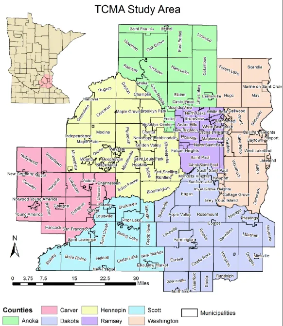
1.1. Study Area

This study will focus on the Twin Cities (Minneapolis and St. Paul) Metropolitan Area of Minnesota. In particular, the study area consists of seven counties: Anoka, Carver, Dakota, Hennepin, Ramsey, Scott, and Washington counties (Figure 1.1). These

counties have a combined area of about 2,939 square miles. From 2000 to 2010, the population increased from 2.6 million to 2.8 million, which comprised approximately 54% of the total population of Minnesota (Metropolitan Council 2000; US Census 2013). At the center of the TCMA are the cities of Minneapolis and St. Paul. St. Paul is the capital of Minnesota, which has a distinct culture from Minneapolis. There are many populous suburbs, as well as highly commercialized areas. The Mall of America, one of the largest indoor shopping centers in the United States (US) is located in Bloomington, south of Minneapolis. Another large shopping mall, the Southdale Center in Edina, is considered the oldest mall in the US. Several major corporations and Fortune 500 companies, such as Target Corporation in Minneapolis, The Toro Company in Bloomington, Dairy Queen in Edina, 3M in Maplewood, and General Mills in Golden Valley, are headquartered in the Twin Cities.

A large part of the early economy of the Twin Cities was influenced by the presence of the Mississippi River and its Saint Anthony Falls, providing hydropower to sawmills and later flourmills. These facilities at Saint Anthony Falls were some of the first to use hydropower in the US (Anfinson 1995). The area was also a major transportation hub for rail and water cargo and passenger services. Grain was a common good to be shipped into the Twin Cities via river or rail, and consequently, flour and other

(16)

milling products were then exported. Timber harvested in Minnesota was also an important shipping good. Manufacturing followed to be a major part of the Twin Cities economy. Today, the economy is dominated by tertiary sector businesses, high-tech research and production, and financial services.

The landscape of the study area is relatively diverse, with a large number of lakes. High density urban development is mostly located in the central part while vegetated land cover and agricultural land are found in the outer perimeter. The maps and data produced in this study will elaborate specific patterns of these land cover classes. The climate in the Twin Cities is typical of the Midwestern US with extreme cold temperatures in the winter and extreme heat in the summer. Precipitation peaks in the summer months. The area is prone to many types of natural disasters, such as tornadoes and other wind storms, flash flooding, extreme temperatures, and winter storms.

The Twin Cities have been found by a variety of surveys over the last years to be one of the most attractive metropolitan areas in the US, and one of the best places to live. These ratings were in large parts due to the proximity to natural features such as lakes, the extensive parks and trails system, and the robust economy.

(17)

(18)

2. Literature Review

This study is concerned with the accurate extraction of impervious surface data and LULC classes from high-resolution aerial imagery and other data sources. The following will give an overview of the existing literature that is pertinent to the various techniques used here. I will first discuss the importance of imperviousness and some techniques that have been used to identify impervious surface areas. I will further give an overview of the research that has been done in relation to the various components of this study, such as data integration, decision tree modeling, and object-based classification.

2.1. Land use and land cover

Land use and land cover data are essential inputs and tools for local and regional decision makers. While urban growth indicates economic growth, it is also a major environmental concern. Urban growth not only leads to increased impervious surfaces and associated problems (see section 2.2), it also significantly degrades air quality at local to global scales, as well as increases energy consumption, and consumes agricultural and forestry resources (Squires 2002). Collinge (1996) conducted a thorough literature review concerning effects of urban sprawl on biodiversity. He concluded that urban sprawl, due to its segmented growth patterns, is a major contributor to habitat fragmentation and therefore reduction of biodiversity. Accurate LULC data are important in order to help decision makers at local, regional, and global scales improve policy

(19)

regarding future development, wetland and habitat conservation, and climate protection (Anderson et al. 1976).

2.2. Imperviousness

The concept and question of imperviousness has received a lot of interest in many fields recently, particularly in geographical and urban studies. Impervious surface restricts the flow of water through the surface. It is often considered to be comprised of rooftops of buildings and transportation features (Schueler 1994); however, it should also be noted that bare, compacted soil or exposed bedrock, at extraction sites for example, may have impervious qualities. In the case of rain events, snow melt, or flooding, water cannot penetrate the ground, but would rather be carried on the surface, picking up many surface pollutants along the way (Chen et al. 2007). Nonetheless, with the increasing dependence on the automobile in the US and other developed and developing countries, the amounts of impervious surfaces and their inherent problems are increasing.

Impervious surfaces accelerate the movement of runoff and pollutants collected over large area, which attributes to many of today’s water pollution problems. As early as 1994, the US Environmental Protection Agency determined that non-point source pollution (of which impervious surface runoff pollution is an example) is the largest contributor and threat to the quality of water in the US (1994). Since non-point source pollutants are carried into surface and ground water, they impact both the natural and human ecosystems.

(20)

Impervious surface is not only a major contributor to non-point source pollution, but also a very good indicator of water quality. Impervious surfaces have been found to be a “key environmental indicator” to estimate many other factors. Arnold Jr and Gibbons (1996) found that knowledge of the amount of impervious surface can serve as a framework for solving problems of natural resource planning. This is particularly advantageous for local planning agencies that may not have the resources to commit more complex studies of particular problematic areas. Impervious surface is not only a general environmental indicator by itself, it is also strongly related to, and can be considered a proxy measure for other indicators that are much harder to measure (Schueler 1994). Impervious surface can be used as a measure of environmental impact not only locally, but also globally, as pointed out by Sutton et al. (2009), who constructed a global model based on satellite imagery and calibrated the model with high-resolution aerial imagery in an effort to show that impervious surface can be a proxy measure for the overall ecological footprint of societies. Although imperviousness has strong impacts on the environment across different scales, it is most powerful at the local scale. As Schueler (1994) noted that impervious surface data are relatively easy to obtain compared to other environmental indicators, and the amount of impervious surface can be managed by local policies.

(21)

2.3. Determining Impervious Surface Area

There are many approaches to estimating the amount of ISA in a study area. Field mapping can be used to achieve accurate results, but is often time-consuming and expensive. Remote sensing techniques offer a more efficient method. Traditional per-pixel approaches classify remote sensing data by assigning land cover classes to each pixel in an image, often based on an algorithm that makes statistical assumptions about the data. To extract impervious surfaces, the image is firstly classified into categories that will allow the researcher to aggregate them into impervious and pervious covers in the next step. For example, urban, transportation, bare soil (such as gravel pits or construction sites), and mining/extraction classes would be considered impervious, while open water, cropland, and wetland classes would be considered pervious. Dougherty et al. (2004) compared this approach to a sub-pixel method. They found that the traditional per-pixel method yielded slightly better results than the sub-per-pixel method, but the accuracy of both methods depended strongly on the types of classified land cover (Dougherty et al. 2004). Lua et al. (2011) described a method that uses the traditional classification method in combination with a segmentation-based method and manual editing to eliminate the drawbacks of each individual method.

Another technique that is relatively prevalent is the use of sub-pixel classifiers to estimate the percentage of impervious surface per area unit, or pixel. This method is based on the use of remote sensing images that have low to medium spatial resolution, which means that a pixel represents a fairly large area on the earth’s surface, and likely comprises many different types of land cover. This method was used by Civco and Hurd

(22)

(1997) to map the amount of impervious surface areas of Connecticut. Their approach involved the use of an artificial neural network, which can be calibrated with high spatial resolution training data, but applied to medium spatial resolution imagery to deliver more accurate results for larger areas. Similar methods were also used by Stocker (1998). Van De Voorde et al. (2009) used two different sub-pixel classification models to extract impervious surface percentages in a comparative study. Similar to Civco and Hurd (1997), they used high spatial resolution images to calibrate their model, and then applied the model to lower spatial resolution images of large areas. They found that the multilayer perceptron model, which is relatively complex to use, performed relatively better than the spectral mixture analysis model. Taking the sub pixel classification approach further, Jennings et al. (2004) developed a model to estimate impervious surface areas, in which various data sources such as the National Land Cover Dataset (NLCD) and municipal transportation layers were used to generate sub-pixel impervious surface maps. These maps were then classified further into conceptual classes describing the amount of impervious surface areas.

A different approach was taken by Ridd (1995) with a “Vegetation – Impervious – Soil” (VIS) model to differentiate urban land cover classes. The model was initially developed for visual interpretation of aerial imagery, but was adapted by Ridd (1995) to be used with digital remote sensing data. The VIS model describes the composition of land based on the three classes it is named for, and can be used with the addition of a water class to determine the amount of impervious surface.

(23)

A modeling method that was not based strictly on remote sensing data was developed by Chabaeva et al. (2004). The authors created a model that can determine the ISA based on population parameters derived from US Census data. They built the model using NLCD shapefiles and created a regression model using inductive learning software. They calibrated the model for different localities and were able to determine the percentage of ISA fairly accurately, however only to the Census tract level (Chabaeva et al. 2004).

After reviewing the literature regarding the extraction of impervious surface, it becomes clear that this topic still has many open questions in terms of which method delivers the most accurate results. Every method described has its own advantages. The method used should be chosen based on the desired results and the available data.

2.4. Data integration

Most of the previously discussed methods of impervious surface extraction mostly only used one specific set of data as their input, such as satellite or aerial imagery, or census and parcel data. Some studies, however, used more than one type of data to extract land cover or impervious surface information for an area. More specialized methods are required, however, to classify using a combination of imagery and more abstract ancillary data types.

For example, Kontoes et al. (1993) described a method using SPOT imagery and ancillary map data that was manually digitized and edited. The authors than employed data derived from both the imagery and the ancillary data in a knowledge-based system

(24)

that allowed them to classify the data and extract agricultural crop coverage with relatively high accuracy. In another approach, McNairn et al. (2005) combined several types of imagery to extract the desired data. They employed and compared the maximum likelihood and decision tree methods. They reported that a decision tree approach allows for the integration of additional data that is not imagery.

Mesev (1998) described a method to extract urban land cover information by combining imagery with census data. However, unlike Kontoes et al. (1993), who employed a knowledge-based model, he was able to integrate the additional data in a maximum likelihood classifier (MLC).

An approach that integrates reflectance data with surface temperature data derived from Landsat data was taken by Lu and Weng (2006). In this case, the researchers used an imagery product and a derivative of the additional infrared emission layer that is delivered with Landsat TM data. Researchers have also combined optical remote sensing with active remote sensing products such as Radar imagery to improve results of classifications. Rignot et al. (1997) compared classifications of a site in Brazil rainforest obtained from the SIR-C radar data and the optical Landsat TM, SPOT, and JERS-1 sensors. They found that each sensor had specific strengths and weaknesses. They were able to combine these results to obtain an overall more accurate final map to identify biomass in their study area. Saatchi et al. (1997) also used radar data to map deforestation in the Brazilian rain forest. They used Landsat TM data to verify their results and also combined their results derived from both data to improve the overall accuracy of their classification. Optical and radar remote sensing data complement each other and

(25)

therefore can improve accuracy, and that radar data can be used where optical data shows weaknesses due to cloud cover or layered vegetation.

2.5. Decision Trees

Decision tree modeling is an artificial intelligence and machine learning technique, as demonstrated by Breiman (1984) and Wu and Kumar (2009). In this study, a combination of the object-based classification, integration of various data sources and types, and decision tree classifier was used. The decision tree software is a machine learning program that analyzes existing data and builds a decision tree model that fits the data best into predetermined classes. Decision trees are used not only for image classification, but also for many other applications in various fields. In general, they are useful for analyzing case data based on specific attributes and assigning discrete output values to each case (Mitchell 1997). There are many medical studies that use decision tree models: Granzow et al. (2001) used decision trees to find relationships between types of tumors and genetic properties. In a different application in cancer research, Kuo et al. (2002) built a decision tree model that could be calibrated to find patterns of breast tumors in different types of ultrasound data. Silva et al. (2003) used decision tree models to classify large amounts of data found in Intensive Care Unit databases to help doctors predict the likelihood of organ failure for patients.

Decision trees have also been used in economics studies to help in making decisions for the creation of stock portfolios (Tseng (2003). Sen and Hernandez (2000) created a decision tree model that helped apartment buyers analyze the various data about

(26)

the apartments and real estate markets that is publicly available, and make better buying decisions based on these data. Arditi and Pulket (2005) were able to use decision tree models to predict the outcome of construction litigation. Another interesting example of decision tree models for real-world applications was presented by Copeck et al. (2002) with their machine learning process to summarize documents.

2.5.1. Decision Trees in Geography

In Geographical studies, decision trees are most often used for image classification, but have also found some other applications: Lang and Blaschke (2006) used a decision tree model to identify the best suited locations for wildlife bridges to protect brown bear habitat in Slovenia. Hansen et al. (1996) described decision trees as an alternative to traditional land cover classifiers and found that they have similar accuracy to Maximum Likelihood Classification, while offering more flexibility for the requirements of input data. Gahegan (2000) examined the particular advantages and disadvantages of using machine learning algorithms to analyze geographical data, as compared to the more traditional statistical tools used in many studies. He also suggested that machine learning tools are often better suited to cope with the very large datasets now used in Geography (Gahegan 2000, 2003). A general comparison of traditional classifiers, artificial neural networks (ANN), and decision tree classifiers was presented by Pal and Mather (2003). The researchers found that decision tree classifiers have advantages over the traditional classifiers since they can handle various types of data on different scales and units, and do not depend on statistical assumptions about the data. In comparison to artificial neural networks, they found that decision trees are advantageous

(27)

because they are easier to use, require less training and parameters to be setup, process large sets of data quickly, and are widely available on the internet. They also found that the decision tree delivered acceptable results compared to other classifiers in most cases (Pal and Mather 2003). In contrast, Rogan et al. (2008) and Rogan et al. (2003) found that ANN can achieve better accuracies for land cover change mapping.

Some good examples of decision tree applications for very large datasets are presented in the publications regarding several US nationwide land cover datasets. Decision tree classifiers were used in building a database of 22 land cover classes with remote sensing data from 2000 and 16 classes with data from 2001 for the entire United States (Homer et al. 2007; Homer et al. 2002). Furthering the use of these datasets, Fry et al. (2009) used decision tree models to map the differences between the 1992 and 2001 National Land Cover Database products efficiently. Another nationwide product that was developed with decision tree models is the 2009 Cropland Data Layer (Johnson and Mueller 2010).

An additional advantage of decision tree classification is that it is able to handle many attributes, or sets of data, and identify the most important ones. This is exemplified by Bricklemyer et al. (2007) to verify the association of agricultural practices with soil carbon sequestration. Similarly, Ban et al. (2010) used decision trees to combine Quickbird and Radarsat data to aid in urban land cover classification. Zhang and Wang (2003) also used decision tree models to classify urban land cover types from high-resolution multispectral imagery. Another study used two types of imagery (medium spatial resolution Landsat and high spatial resolution aerial imagery) to estimate the

(28)

density of tree cover for large areas (Huang et al. 2001). Instead of utilizing two sources of imagery, Harris and Ventura (1995) used Landsat imagery and more abstract geographical data, such as parcel and census data, to classify urban land cover types. In contrast, Griffin et al. (2011) used decision trees to include environmental factors in a classification of various vegetation types in a specific ecosystem. For a study to assess animal habitats and agricultural land cover, Lucas et al. (2007) employed a rule-based decision tree to map the habitats and cover classes based on multi-temporal satellite imagery, various derivatives of the imagery, and data retrieved from an agricultural management system. A similar approach was taken by Wright and Gallant (2007) to increase the accuracy of wetland mapping in Yellowstone National Park.

In addition to all of the previously mentioned advantages of decision tree modeling, another benefit of this technique is its ability to deal with errors very well (Mitchell 1997). Two major error sources in remote sensing are uncertainties already present in the imagery due to acquisition and processing issues, and errors introduced by the analyst while generating training data (Foody et al. 2002). Decision tree models are particularly tolerant towards both of these error types, and can even handle cases where some of the attributes are missing very well (Mitchell 1997).

It is evident that decision tree classification systems can deliver accurate results for many different applications in geographic research, particularly when dealing with datasets that are either very large, contain different data scales or units, or are problematic for traditional or statistical models. Decision trees are found to be flexible, user-friendly, and efficient.

(29)

2.5.2. Decision Trees for Impervious Surface Extraction

Studies that used decision trees to identify ISA only have emerged in the past ten to fifteen years. Smith (2000) employed a decision tree model to estimate the sub-pixel level ISA from Landsat imagery in the diversely urbanized area of Santa Barbara in Southern California. Similarly, Yang, Huang, et al. (2003) and Yang, Xian, et al. (2003) used decision trees to extract sub-pixel ISA from Landsat TM and ETM+ and high-resolution aerial imagery, and to detect urban land cover changes, respectively. High spatial resolution aerial imagery was used by Cutter et al. (2002) to extract ISA. Goetz et al. (2003) used decision trees to extract not only impervious surfaces, but also tree covers from IKONOS imagery.

While decision tree classifiers have been used occasionally to extract impervious surface from medium spatial resolution imagery by means of sub-pixel classification, they seem to be most efficient for use with high spatial resolution imagery. This is noted by Cutter et al. (2002), who found that traditional classifiers are often unable to handle the challenges posed by high spatial resolution imagery. The fact that this high spatial resolution imagery is becoming more widely available may also explain the fact that there has very little work been done for impervious cover extraction with decision trees until recently.

(30)

2.6. Object-based Classification

While a decision tree approach was used in this study to classify ISA, the remaining LULC classification was completed using object-based classification. Object-based classification is a relatively new concept compared to pixel-Object-based classification. Its development began when per-pixel classification was found to be lacking in some aspects, and when computing power increased which allows for the development of more advanced techniques. Tobler (1970) defined the first law of Geography as: “Everything is related to everything else, but near things are more related than distant things.” Therefore, many researchers have criticized the focus on the pixel as a unit in image classifications. They have found that it makes more geographical sense to include not only the information that is present in one pixel, but also what surrounds that pixel. Considering this, one should not only focus on individual pixels in a study, but also should consider the data in their surroundings (Fisher (1997) and Cracknell (1998). Haralick et al. (1973), Haralick and Shapiro (1985), and Myint (2001) all suggested to integrate contextual information by calculating textures based on surrounding pixel values in order to implement this principle in remote sensing applications. In this study, the texture-band approach was followed for the impervious surface classification.

Object-based classification was employed as an additional method of incorporating contextual information. Instead of looking at each pixel individually, this method attempts to find patterns in the pixel values and group pixels according to these patterns. This process is also referred to as image segmentation (Blaschke and Strobl 2001). This approach has been found to be advantageous particularly when classifying

(31)

imagery that has very limited spectral resolution, such as grayscale imagery (Blaschke and Strobl 2001), and for imagery that is problematic to classify because of its high spatial resolution (Miller et al. 2009). While object-based classification is mostly suitable for extraction of certain objects (such as trees, buildings, water bodies), it can be adapted to be used on the extraction of land cover classes based on multi-scale objects (Baatz and Schäpe 2000). In this study, object-based classification was used for the general LULC classification part.

2.7. Feature Analyst

Feature Analyst is the software chosen here to implement the object-based LULC classification. Feature Analyst is a third-party extension for ESRI ArcGIS, and is considered an object-based, inductive learning classification system.

In fact, Feature Analyst is a combination of various classification algorithms. It is object-based because it makes use of image segmentation, and is capable of identifying individual objects in an image, compared to many other systems which can only perform so called “wall-to-wall” classifications where every object within an image has to be included in the classification.

Aside from image segmentation, Feature Analyst makes use of several other classification models. These include: (1) decision trees, (2) variants of ANN, which are designed to assess information in a similar way to the human brain (Opitz and Blundell 2008; Rumelhart et al. 1986), (3) Bayesian learning, which is similar to ANNs, but additionally makes use of probability assumptions about the data, and (4) K-nearest

(32)

neighbor, which attempts to assign a class to a case simply based on how “close” its attributes are to those of known cases (Mitchell 1997). Feature Analyst automatically includes one or more of these approaches in its classification models, depending on which approach is best suited for the data to be classified (Opitz and Blundell 2008).

In addition to selecting one or several classification approaches, Feature Analyst will also make use of ensembles, a concept very similar to boosting in decision trees (see 3.3.2). Ensembles are sets of classification models, which are trained using the same data, and whose results are combined to produce a final result. While there are several options to combine the results, the most common, and the one used in Feature Analyst, is a weighted average of all results (Opitz 1999). Several studies have found that ensemble predictions become more accurate if the individual predictors disagree as much as possible (Breiman 1996; Freund and Schapire 1996; Opitz and Shavlik 1996a, 1996b). Therefore, Feature Analyst actively attempts to build several models that produce diverse results, thus increasing the possible accuracy of the entire ensemble (Opitz and Blundell 2008). This approach is claimed to be more accurate than similar techniques, such as decision tree boosting.

In summary, Feature Analyst makes use of several innovative and advanced image classification techniques that promise improved accuracy for high spatial resolution imagery compared to other, pixel-based classification techniques.

(33)

3. Methods

3.1. Data Acquisition and Preprocessing

The data used in this study were obtained from the United States Geological Survey (USGS) Seamless Data Warehouse website (http://seamless.usgs.gov/), and the Minnesota Geospatial Information Office (MNGEO) Data Clearinghouse (http://www.mngeo.state.mn.us/). The specific datasets were 2010 high-resolution digital ortho-imagery, Light Detection and Ranging (LIDAR) elevation data, and road centerline data.

3.1.1. Aerial Imagery

The aerial imagery was part of the National Agriculture Inventory program (NAIP) funded by the U.S. Farm Services Agency (FSA), which makes these data available for public use at no charge. The 2010 NAIP ortho-images were flown during the agricultural growing season, specifically during the months of July and August. The images have a spatial resolution of 1 meter per pixel, and radiometric resolution of 8 bit pixel depth. The NAIP imagery is ortho-rectified by the data vendor to a horizontal accuracy of +/- 5 meter using ground control points. The vendor further mosaicked the individual images to produce county mosaics using a last-in-last-on-top strategy, and color-balanced the mosaics using the Impho Orthovista software.

The aerial images were acquired as full county mosaics for each of the seven metropolitan counties. Instead of mosaicking these individual files into a new raster, the ArcGIS mosaic dataset functionality was used. A mosaic dataset is a dynamic mosaicking

(34)

and processing tool that allows for images to be mosaicked on the fly, rather than statically. The dataset itself only contains references to the individual files, and is therefore very disk-space efficient. In addition to applying various mosaicking functions, it is also possible to add other raster functions on the fly, for example NDVI, pan sharpening, or hillshade processing for elevation rasters. The major advantages of the mosaic dataset include: it is very fast to apply functions; it reduces the required storage space by avoiding duplication of data; and it is compatible with any ArcGIS raster tools. In this study, the mosaic dataset was used first to mosaic the NAIP images to achieve coverage of the entire study area. A clip function was applied to exclude areas outside of the seven county metropolitan area of interest.

In order to provide additional classification parameters for both the LULC and the impervious surface classification, the near-infrared band of the NAIP imagery was also used to calculate texture values. Texture, when thought of as variance in specific localized parts of the data, has previously been seen as undesirable as it could make classification with per-pixel methods more difficult (Ryherd and Woodcock 1996; Gong and Howarth 1990; Herold et al. 2003; Zhang 1999). This study uses an object-based and a pixel-based decision tree classifier. Texture information is known to be valuable for use in object-based systems (Ryherd and Woodcock 1996), and due to the winnowing function of C5, it can also be used in this pixel-based approach. When texture is specifically used as an input for image classification, especially in segmentation-based processes, it can be beneficial. The texture layer was calculated as variance of a 3x3 pixel window (Yuan 2008). The equation used to calculate variance is as follows:

(35)

Unfortunately, because the functions that can be used with mosaic datasets are predefined, this step could not be performed directly with one function. Chaining of functions in a mosaic dataset allows for several functions to be applied to the data in a specified order. Therefore, variance was implemented by first applying a standard deviation function, and then squaring the result of that function in a separate function. These functions were applied with a 3 x 3 pixel window.

3.1.2. Elevation Data

In addition to aerial imagery, elevation data derived from LiDAR data were utilized. The elevation data used in this study were acquired in 2011 and 2012 by private vendors in cooperation with the Minnesota Department of Natural Resources (MNDNR). These data are part of Minnesota’s statewide Elevation Mapping Project. The Twin Cities Metro Region dataset used here has three different point densities, depending on the area covered: Anoka, Carver, Hennepin, Ramsey, Scott, and Washington counties were sampled at 1.5 points per square meter, Dakota County at 2 points per square meter, and the cities of Minneapolis, St. Paul, and Maple Grove at 8 points per square meter. The MNDNR determined the vertical accuracy to be 5 cm, 10.8 cm, and 8.3 cm for the entire

Equation 3.1: Variance calculation where is the DN value of the pixel at i,j, and is the number of pixels in the window. Adopted from (Yuan 2008).

(36)

metro block area, Dakota county, and Maple Grove, respectively. The data vendor produced a Digital Elevation Model (DEM) from these LiDAR point data based on the terrain-only points. Since the DEM files are provided at the same spatial resolution as the aerial imagery (1 m pixel size), no further processing was necessary. DEM rasters were mosaicked using a mosaic dataset and masked to the same extent as the aerial imagery using a mosaic dataset function.

3.1.3. Road centerline data and Road Density

As an additional dataset, the roads basemap was downloaded from the MNDNR Data Deli website, a statewide geospatial data portal. The purpose of the roads layer in this study was the production of a road density layer. The roads layer is a digitized map of roads, produced by the Minnesota Department of Transportation (MNDOT). Roads were digitized based on 7.5 minute USGS quadrangle topographic maps, and was updated in 2001. The horizontal accuracy of these roads is less than +/- 12 m. Roads are represented as centerlines, and detailed road class information is given.

3.1.4. Additional supporting data

In addition to the aforementioned data that were used directly in creating the classification maps, ancillary datasets were acquired to support the analysis and interpretation of the results. First, political boundary polygonal shapefiles were acquired for the county and municipality levels. County boundaries were retrieved from the MNGeo Geographic Data Clearinghouse online (http://www.mngeo.state.mn.us/). These boundaries were current as of June 2013. They are represented at a nominal scale of

(37)

1:24,000, and have a spatial accuracy of +/- 12 meters (40 feet). Similarly, boundaries of all municipalities were also retrieved from MNGeo. These boundaries have the same temporal and spatial characteristics as the county boundaries, and include cities, townships, and unorganized territories (CTUs). It should be noted that the township boundaries refer to political entities, which do not necessarily coincide with public land survey entities.

In addition, the US Census Factfinder website (http://factfinder2.census.gov) was used to acquire population data for the area and the political entities represented in the previously mentioned boundary files.

3.2. Land use and land cover classification

The LULC classification was performed using Feature Analyst, an extension for ArcGIS that employs a proprietary, object-based, inductive learning classification algorithm. Before conducting the classification, the class scheme was determined. The extracted LULC classes include water (rivers, lakes, pools, and other open bodies of water), urban impervious infrastructure (roads, buildings), cropland (non-vegetated and vegetated fields and pasture), forested areas (deciduous, evergreen, and mixed forests), other vegetated areas (shrub, herbaceous plants, non-forested wetlands), and bare soil and rock (mining operations such as gravel pits, bedrock). An important note to be made is that the cropland class was classified in two steps: first, it was separated into the vegetated and non-vegetated parts of cropland, and then these two classes were merged to form one class. These steps were taken due to the bi-modal distribution of spectral values

(38)

within this class. While object-based classification methods should be better at coping with this issue than traditional pixel-based approaches, initial testing showed that this step increases classification accuracy for cropland class by avoiding its confusion with other LULC classes.

Object-based classification in Feature Analyst makes use of the inductive learning approach. This means that the algorithm relies on an expert, or teacher, to identify examples of the desired outcome in the imagery, therefore providing a set of training data to the classification system. The algorithm then uses the information contained in these samples to build the model which is used to perform the classification. Training samples had to be determined manually based on a set of criteria for each class. The classifier not only relies on spectral information contained in each pixel, but also considers information derived from pixel groups. This is based on a process known as image segmentation, which divides the individual pixels into groups, representing objects. The segmentation is generally based on homogenous pixel values, edges, and shapes. After defining these objects, additional information from training data is used to determine which class an object belongs to. Spectral values, along with additional data such as the size and shape of the object, and its patterns, texture, and neighboring objects are used to assign class values. Accordingly, training samples had to represent all of these characteristics for each class. Training samples were created as polygons, and were drawn as close to the edge of each feature as possible to allow the sample to represent the shape and edge type of the object. For example, most buildings are relatively simple, rectangular features, while rivers or lakes have more complex, curved outlines which were indicated by the shape of

(39)

their training polygons. Care was also taken to include the full variety of each feature found in the study area. For example, small outbuildings, residential homes, and large commercial or industrial facilities were all included in the urban training set to appropriately represent the range of sizes and shapes of this object type within the study area.

After creating the training polygon set, Feature Analyst presents several other settings that are used during the classification process to adjust the algorithm for the specific situation and improve its accuracy. First, input data are defined. Feature Analyst allows the use of multiple sets and types of data. Therefore, the LULC classification was based on the four band NAIP imagery from 2010, along with the LiDAR-derived elevation data and a texture layer. This is possible in Feature Analyst without previously stacking or otherwise altering the input layers; they are simply added to a list of inputs, and their type (i. e. optical, elevation, texture) is defined. Since Feature Analyst is capable of extracting individual features or perform complete, exhaustive and inclusive classifications of land cover features, there are several other options available. First, the “wall-to-wall” option was selected to force Feature Analyst to classify all areas of the imagery, rather than just extracting some features. Feature Analyst is also able to automatically stretch the image data, however, this options was disabled because the data were already stretched on-the-fly by the mosaic dataset functions. In order to make use of contextual information (i. e. analyze objects based on their neighboring objects), Feature Analyst uses a system called input representation. These representations are essentially local windows which let the classifier see more than one pixel at a time during

(40)

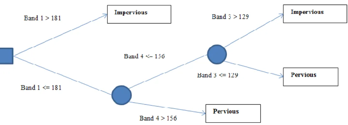
processing. This allows the classifier to build its model based on not only one pixel, but also its neighboring pixels. However, this approach increases the amount of processing time required to build and implement the model, and it still only takes into account a relatively small areas surrounding each pixel. Feature Analyst allows for more complex window patterns, which are known as foveal representations, as they are designed to mimic the way the human eye sees things (Opitz and Bain 1999). Figure 3.1 shows an

example of these foveal representations used in Feature Analyst, the Manhattan pattern. Colored pixels are those that would be visible to the classifier while analyzing the center pixel, while uncolored pixels would be ignored. Compared to simple local windows, this approach allows the classifier to give more importance to pixels nearer to the pixel being processed, yet take into consideration information found in pixels further away as well. This approach should increase the amount of information available to the classifier, while at the same time not increasing the amount of data to be processed as much as the simple window approach. This approach makes the integration of contextual information in a classification model more efficient, and again is a testament to Tobler’s First Law of Geography, which states that near things are more related than distance things (Tobler 1970).

(41)

3.3. Impervious surface classification

3.3.1. Road Density

Road density is often considered an important measure of urbanization (Schueler 1994). Therefore, road density was computed as a raster surface to be used as one of the input parameters for the impervious surface decision tree modeler. Road density is generally defined as kilometers of road per 100 square kilometers of area, or miles of road per square miles of area. To make the data processing more manageable and to ensure that road density was considered locally rather than globally for the entire study area, it was calculated for an area of 1 square kilometer around each pixel. The road density calculation was conducted based on the road centerline layer. The density was calculated as meters of roads per square kilometer of area, and stored in a floating point raster with 1 m pixel size. The resulting data were used as input parameters for the decision tree model.

(42)

3.3.2. Decision Tree Modeling

Impervious surface was classified using a decision tree classifier. Specifically, the See5 software was used to generate the decision tree based on the C5 algorithm (Quinlan 2013a). C5 is very similar to the C4.5 algorithm, with the addition of several features that have the potential to increase the classification accuracy (Quinlan 1993, 2013b).

In general, C4.5 and C5 are expert-knowledge systems that require human inputs in the form of training data. The general purpose is to use the training data to identify to which class each case should belong, and then find an accurate model representation to assign a class to each case in the general population based. To achieve this, C4.5 and C5 algorithms begin by dividing the cases based on their attributes and then identify a natural break-point in the attribute based on the class value. This approach produces a set of decision rules that can be combined to build a tree consisting of branches and leaves. Each branch represents a test that is performed on the data, and leads to either a further branch, or a leaf, where a decision is reached and a class assigned. These steps are performed automatically by the C5 algorithm. In addition, C5 can perform winnowing (decide to exclude attributes if they do not significantly contribute to the model) and pruning (removing branches that do not significantly contribute to the model) (Quinlan 1993, 2013a, 2013b).

In order to create training data for the decision tree model, a set of 300 randomly distributed points was created. A second set of points following the same principle was created to be used for accuracy assessment (Congalton 1988). Both sets were created at this time because C5 is able to conduct the accuracy assessment automatically after

(43)

generating the model based on a separate set of points. Therefore, the accuracy of the decision tree model could be evaluated immediately, and the algorithm configuration could be adjusted if necessary. For each set of points, the ArcGIS “Value to points” tool was used to write raster values to the attribute table for each point. The values of each band of the aerial imagery, the calculated texture layer, elevation raster, LULC raster, and road density map were included in this process. A field containing binary impervious surface data was added and populated by visually determining whether each point is located on impervious surface or not. The resulting tables were then adjusted in Microsoft Excel and exported for use in See5.

In See5, the data were analyzed several times using different options to identify the settings that can deliver the best accuracy and efficiency. Specifically, the winnowing, pruning, and boosting options were evaluated. Winnowing prompts See5 to evaluate the impact of each attribute on the final model and decide whether it should be used or not. This aids in faster processing and makes the resulting decision tree smaller and less complex, often leading to better accuracy (Quinlan 1993; Foody et al. 2002). Pruning is also a method of making large decision trees smaller and less complex. When pruning is used, the tree is first produced normally, and then pruned. Pruning works by dividing the tree into several subtrees and estimating the likelihood of misclassification for each subtree. This estimation is then compared to the case where the subtree would simply be replaced by a leaf. If this change does not change the likelihood of misclassification by more than a certain threshold, the change is committed to the tree; otherwise, the subtree is left the way it is (Quinlan 1993). Pruning is useful to improve

(44)

trees that suffer from over fitting, a condition where the decision tree fits the training data almost perfectly, but is biased to these data, and therefore fails to accurately model the test or accuracy assessment data (Foody et al. 2002).

Boosting is a method that is used only to increase the accuracy of decision trees, at the cost of making the model more complex and computationally expensive. Boosting works by creating more than one model to solve the same problem and using the results from each model to “vote” for a final result (Freund et al. 1999; Quinlan 2013b; Schapire 1999). For example, if ten models are created to classify pixels, and six of them determine a pixel to be in class a, while four assign class b, the final result would be the majority vote, class a.

The See5 output is a text file representing the decision tree in a pseudo-graphical way. This model was manually “translated” to be used in a Python script to carry out the actual data processing. The script makes use of the ArcGIS ArcPy module, which allows the use of ArcGIS tools within a Python script.

The decision tree was implemented in the script by using a series of nested “Con” conditional statements from ArcGIS Spatial Analyst. The Con function evaluates a condition on a per-pixel basis, and can either output a constant, another raster value, or initiate another con statement nested within it. Some of the advantages of implementing this function in a Python script is that it is easily possible to save and adjust the script at any time, and that operations can be performed in memory rather than from the hard drive, therefore improving performance. The use of ArcPy also makes it possible to utilize ArcGIS mosaic datasets as inputs, rather than statically mosaicked raster files.

(45)

While it would be possible to process the decision tree model in Python without using ArcPy components, this would only work with fully mosaicked raster files. Therefore, by using mosaic datasets instead, an additional processing and data intensive step is cut from the workflow. After processing the decision tree based on the defined input layers, the result was written to disk as a 1-bit raster file. Impervious surface was classified using this newly developed decision tree model. Specifically, to build the model, the algorithm had access to the following attributes for each case (sample pixel): the four-band NAIP aerial imagery, the LIDAR DEM, the texture layer generated from the near infrared band of the aerial imagery, the road density layer, and the LULC raster map. While building the decision tree model, several advanced options were evaluated in terms of their ability to increase the classification accuracy of the model. These options are specifically winnowing, pruning, and boosting (see 3.3.2). It was found that the use of winnowing did not make a difference in the model. See5 used the same attributes whether winnowing was used or not. Therefore, winnowing was not used for the final model. Further, the decision tree model created without pruning was already relatively small and had very good accuracy. Pruning the tree did not reduce its size enough to justify the loss in accuracy caused by the use of pruning. For the boosting options, a manageable amount of ten trials was evaluated. It was found that using boosting with ten models did not increase accuracy enough to justify the additional complexity and computational expense of the resulting model. In fact, while accuracy increased for the training dataset, boosting decreased the accuracy attained for the test dataset. Based on these evaluation results, the basic decision tree without advanced options was chosen as the final model.

(46)

The final decision tree model only includes bands one, three, and four from the aerial image. The decision tree consists of two branches and four leaves (see Figure 3.2).

3.4. Accuracy Assessment

An accuracy assessment was conducted on both the LULC and impervious surface maps independently. For each map, a set of 300 random sample points was created (Congalton 1988, 1991b). Reference values assumed to be “ground true” were assigned to these points based on visual inspection of the imagery. To determine the classified values for the LULC map, the ArcGIS “Value to points” tool was used to automatically write raster values from the LULC map to the sample point table. For the impervious surface, this task was achieved by See5, which allows for the input of a separate set of accuracy assessment data and automatically evaluates the model against these data.

(47)

Standard accuracy matrices were generated for both maps, and per-class user’s and producer’s accuracy, overall accuracy, and estimated Kappa accuracy were calculated based on the matrices (Cohen 1960; Bishop et al. 1975; Congalton 1991a; Congalton and Mead 1983). User’s accuracy is also referred to as error of commission, which describes classification errors where a pixel that belongs to one class was falsely assigned to a different class. In contrast, producer’s accuracy or error of omission is an error where a pixel that should have been assigned a certain class value, but was not included in that class (Campbell 2002). The Kappa statistics were estimated with an equation given by Cohen (1960) (see Equation 3.2). Cohen’s Kappa is also referred to as inter-observer agreement, and originated in Psychological studies (Cohen 1960). The Kappa coefficient was first proposed by Congalton and Mead (1983). estimates “the difference between the observed agreement between two maps […] and the agreement that might be attained solely by [chance]” (Campbell 2002).



          _r i i i r i r i i i ii

x

N

x

N K 1 2 1 1 ˆ

(48)

4. Results

4.1. Land use and land cover classification

4.1.1. LULC: Entire study area

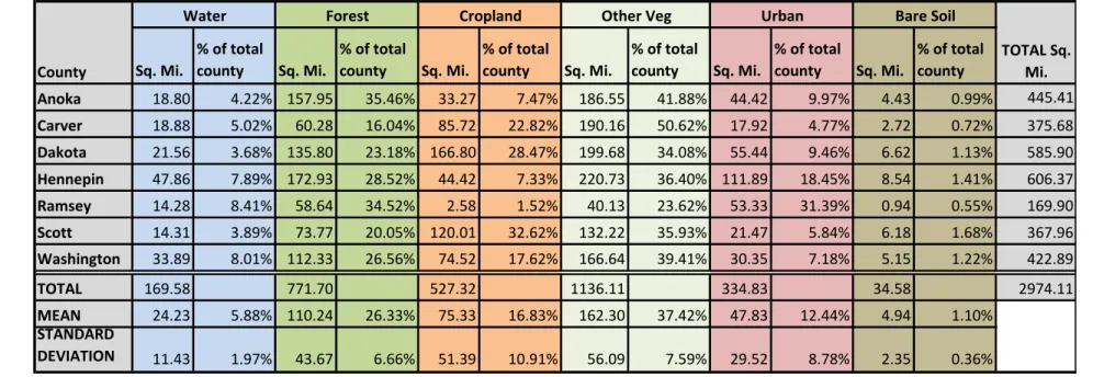
Land use and land cover distribution was first determined and analyzed for the entire study area without further subdividing into political entities. Table 4.1 shows the

area of each LULC class by county as well as total values. The largest LULC class in the study area was other vegetation, which had a total area of 1136 sq. miles, or 38.2% of the entire study area. This was followed by forest (772 sq. mi, 26%), cropland (527 sq. mi, 17.7%), urban (335 sq. mi, 11.3%), and water (170 sq. mi, 5.7%). The smallest class was bare soil, which only made up 34.6 sq. miles or 1.1% of the entire study area.

(49)

Table 4.1: LULC area by county. Sq. Mi. % of total county Sq. Mi. % of total county Sq. Mi. % of total county Sq. Mi. % of total county Sq. Mi. % of total county Sq. Mi. % of total county Anoka 18.80 4.22% 157.95 35.46% 33.27 7.47% 186.55 41.88% 44.42 9.97% 4.43 0.99% 445.41 Carver 18.88 5.02% 60.28 16.04% 85.72 22.82% 190.16 50.62% 17.92 4.77% 2.72 0.72% 375.68 Dakota 21.56 3.68% 135.80 23.18% 166.80 28.47% 199.68 34.08% 55.44 9.46% 6.62 1.13% 585.90 Hennepin 47.86 7.89% 172.93 28.52% 44.42 7.33% 220.73 36.40% 111.89 18.45% 8.54 1.41% 606.37 Ramsey 14.28 8.41% 58.64 34.52% 2.58 1.52% 40.13 23.62% 53.33 31.39% 0.94 0.55% 169.90 Scott 14.31 3.89% 73.77 20.05% 120.01 32.62% 132.22 35.93% 21.47 5.84% 6.18 1.68% 367.96 Washington 33.89 8.01% 112.33 26.56% 74.52 17.62% 166.64 39.41% 30.35 7.18% 5.15 1.22% 422.89 TOTAL 169.58 771.70 527.32 1136.11 334.83 34.58 2974.11 MEAN 24.23 5.88% 110.24 26.33% 75.33 16.83% 162.30 37.42% 47.83 12.44% 4.94 1.10% STANDARD DEVIATION _11.43 _1.97% _43.67 _6.66% _51.39 _10.91% _56.09 _7.59% _29.52 _8.78% _2.35 _0.36% Bare Soil County TOTAL Sq. Mi.

(50)

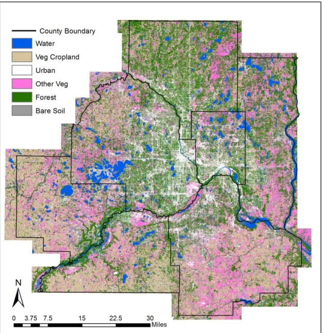
The final 1 m LULC classification map is shown in Figure 4.1. Because of the

high spatial resolution of the classified map and the relatively large size of the study area, some of the more detailed analysis is lost when the map is viewed in its resampled form showing the entire study area. In order to better analyze the patterns of each LULC class, the data were aggregated into a regular, hexagonal grid (see Figure 4.2). Each hexagon

has a side length of 1 km, giving it an area of approximately 1 sq. mile. The major roads shown are Interstate and Minnesota State highways, and are included for reference purposes. In order to identify spatial patterns of LULC classes, individual maps were created for each class. In addition, hot and cold spots and clustering of the features were evaluated using Getis-Ord G* and Moran’s I statistics, respectively. Getis-Ord G* generates a z-score that indicates hot spots (clustering of high values) and cold spots (clustering of low values). The equation is indicated in Appendix B. Getis-Ord G* outputs a map that further indicates areas of high or low concentration of each LULC type and aids in identifying patterns of spatial distribution (see Figure 4.3). As it is assumed that most of the LULC features are clustered in certain areas, the Moran’s I statistics was used to verify this assumption. The equation is given in Appendix A. Global Moran’s I statistics are given for each class in Figure 4.3. The Moran’s I statistics

for all LULC classes have p-values of 0 and z-scores much larger than the critical value of 2.58 (for a confidence interval of 0.99). Therefore, it can be assumed that the LULC patterns are not randomly distributed. Further, all classes exhibit a positive Moran’s I index value, therefore indicating a tendency towards clustered distribution.

(51)

The urban LULC class exhibits a pattern of high density towards the center of the study area, and gradually decreasing density towards the outer edges. There are, however, several smaller, outlying clusters of urban cover found in the outer perimeter. These clusters likely show locations of smaller towns surrounding the major metropolitan area