Southern Methodist University Southern Methodist University
SMU Scholar
SMU Scholar
Electrical Engineering Theses and Dissertations Electrical Engineering
Fall 12-21-2019
Technology-dependent Quantum Logic Synthesis and Compilation
Technology-dependent Quantum Logic Synthesis and Compilation
Kaitlin SmithFollow this and additional works at: https://scholar.smu.edu/engineering_electrical_etds
Part of the Other Electrical and Computer Engineering Commons Recommended Citation
Recommended Citation
Smith, Kaitlin, "Technology-dependent Quantum Logic Synthesis and Compilation" (2019). Electrical Engineering Theses and Dissertations. 30.
https://scholar.smu.edu/engineering_electrical_etds/30
This Dissertation is brought to you for free and open access by the Electrical Engineering at SMU Scholar. It has been accepted for inclusion in Electrical Engineering Theses and Dissertations by an authorized administrator of
TECHNOLOGY-DEPENDENT QUANTUM LOGIC SYNTHESIS AND COMPILATION
Approved by:
Dr. Mitchell Thornton - Committee Chairman Dr. Jennifer Dworak Dr. Gary Evans Dr. Duncan MacFarlane Dr. Theodore Manikas Dr. Ronald Rohrer
TECHNOLOGY-DEPENDENT QUANTUM LOGIC SYNTHESIS AND COMPILATION
A Dissertation Presented to the Graduate Faculty of the Lyle School of Engineering
Southern Methodist University in
Partial Fulfillment of the Requirements for the degree of
Doctor of Philosophy with a
Major in Electrical Engineering by
Kaitlin N. Smith
(B.S., EE, Southern Methodist University, 2014) (B.S., Mathematics, Southern Methodist University, 2014)
(M.S., EE, Southern Methodist University, 2015)
ACKNOWLEDGMENTS
I am grateful for the many people in my life who made the completion of this dissertation possible. First, I would like to thank Dr. Mitch Thornton for introducing me to the field of quantum computation and for directing me during my graduate studies. I would also like to thank my committee for supporting my research and for all of the suggestions and guidance that helped me to develop my skills as a scientist.
To my family and friends: thank you for being there. You have no idea how much your constant encouragement, advice, and love have meant to me over the years as I completed this degree.
To my Mom and Dad: thank you for always being my biggest fans and for always believing in me. You have both taught me so much, and have given me the courage to chase my dreams. I love you.
Smith , Kaitlin N. B.S., EE, Southern Methodist University, 2014
B.S., Mathematics, Southern Methodist University, 2014 M.S., EE, Southern Methodist University, 2015
Technology-dependent Quantum Logic Synthesis and Compilation
Advisor: Dr. Mitchell Thornton - Committee Chairman Doctor of Philosophy degree conferred December 21, 2019 Dissertation completed September XX, 2019
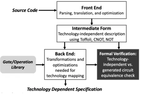
The models and rules of quantum computation and quantum information processing (QIP) differ greatly from those that govern classical computation, and these differences have caused the implementation of quantum processing devices with a variety of new technologies. Many platforms have been developed in parallel, but at the time of writing, one method of quantum computing has not shown to be superior to the rest. Because of the variation that exists between quantum platforms, even between those of the same technology, there must be a way to automatically synthesize technology-independent quantum designs into forms that are capable of physical realization on a quantum computer (QC) with specific operating parameters. Additionally, results of synthesis must be formally verified to con-firm that output technology-dependent specifications are logically identical to their original, technology-independent forms. The first contribution of this work to the field of quantum computing is the creation of such a methodology. Quantum technology mapping and op-timization for machines with fixed coupling maps and libraries of gates can be performed with an automatic quantum compiler, and the development and test of this compiler will be explored in this dissertation. Furthermore, this compiler can be considered in a more general context to be a synthesis tool for QIP circuits in a specific realization technology, many of which are capable of implementing systems where the radix of computation, r, is greater than two. As a result of this ability, the second contribution of this work is the presentation of architectures for higher-dimensional quantum entanglement.
TABLE OF CONTENTS
ACKNOWLEDGMENTS . . . iii
LIST OF FIGURES . . . viii
LIST OF TABLES . . . x
LIST OF ABBREVIATIONS . . . xii
CHAPTER 1. Introduction . . . 1
1.1. Classical Computation and Limitations . . . 2
1.2. Contribution . . . 3
2. Quantum Information . . . 4
2.1. The Qubit . . . 4
2.2. Physical Quantum Implementations . . . 6
2.2.1. Transmons . . . 7
2.2.2. Photonics . . . 8
2.3. The Superposition Principle . . . 10
2.4. The Wavefunction and Quantum Computing . . . 11
2.5. Quantum Operations . . . 14
2.6. Requirements for Quantum Computation . . . 17
2.7. Entanglement . . . 18
3. Quantum Logic Synthesis Considerations . . . 22
3.1. No-Cloning Theorem . . . 22
3.2. Reversible Logic . . . 24
3.3. Gate Libraries and Coupling Constraints . . . 26
3.4.1. IBM Q. . . 27
3.4.2. Rigetti . . . 29
3.4.3. Quantum with Photonic Devices . . . 30
3.5. Quantum Cost . . . 33
3.6. Quantum Multiple-valued Decision Diagrams . . . 35
3.7. Zero-supressed Decision Diagrams . . . 36
4. Technology Mapping Algorithms . . . 39
4.1. Connectivity Tree Reroute . . . 39
4.2. Zero-suppressed Decision Diagram Technology Mapping . . . 42
4.2.1. Problem Formulation with ZDD Mapping . . . 42
4.2.2. Finding Maximal Partitions . . . 43
4.2.3. ZDD mapping in the Quantum Compilation Flow . . . 47
4.2.4. Experimental Results . . . 48
5. Formally-verified Synthesis Methods and Experiments . . . 52
5.1. IBM . . . 53 5.1.1. Methodology . . . 53 5.1.2. Experimental Results . . . 55 5.2. Rigetti . . . 62 5.2.1. Methodology . . . 62 5.2.2. Experimental Results . . . 65
6. Higher Dimensioned Quantum Logic Synthesis . . . 68
6.1. Qudit Information . . . 71
6.2. Qudit Superposition . . . 73
6.2.1. The Hadamard Gate . . . 74
6.3. Single Qudit Basis Permutation . . . 78
6.4. Controlled Qudit Operators . . . 79
7. Higher Dimensioned Entanglement Generators . . . 84
7.1. Partial Entanglement of Qudit Pairs . . . 85
7.2. Maximal Entanglement Generators for Qudit Pairs . . . 87
7.3. Maximal Entanglement of Qudit Groups . . . 97
7.3.1. Synthesis of Qudit Entanglement States . . . 100
8. Conclusion . . . 106
8.1. Summary . . . 106
8.2. Future Work . . . 107
APPENDIX A. The Radix-4 Chrestenson Gate . . . 109
A.0.1. Quantum Optics . . . 110
A.1. The Four-port Coupler . . . 111
A.2. Physical Realizations of the Four-port Coupler . . . 115
A.2.1. Fabrication . . . 117
A.2.2. Characterization . . . 117
LIST OF FIGURES
Figure Page
2.1 The Bloch sphere . . . 5
2.2 Photonic transformation between polarization and dual-rail encoding schemes . 9 2.3 Quantum circuit example 1. . . 17
2.4 Bell state generator . . . 20
3.1 Proposed qubit copying gate, G. . . 22
3.2 Boolean AND and OR operation symbols and truth tables . . . 25
3.3 Representation of CNOToperation as a QMDD.. . . 36
3.4 A ZDD representing the family of sets{{x1, x2},{x1, x3},{x1, x4},{x2, x3},{x2, x4},{x3, x4}}. All internal non-terminal nodes are annotated with the sets they repre-sent. Dashed edges indicate LO and solid edges indicate HI. . . 38
4.1 Implementation of SWAP operation usingCNOT. . . 39
4.2 CNOT orientation reversal.. . . 40
4.3 Pseudocode CTR algorithm.. . . 41
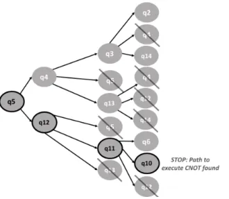
4.4 CTR implementation on theibmqx3 machine for a CNOTwith q5 as con-trol and q10 as target. . . 41
4.5 Algorithm: Find maximal partitions. . . 45
5.1 Synthesis and compilation tool architecture. . . 52
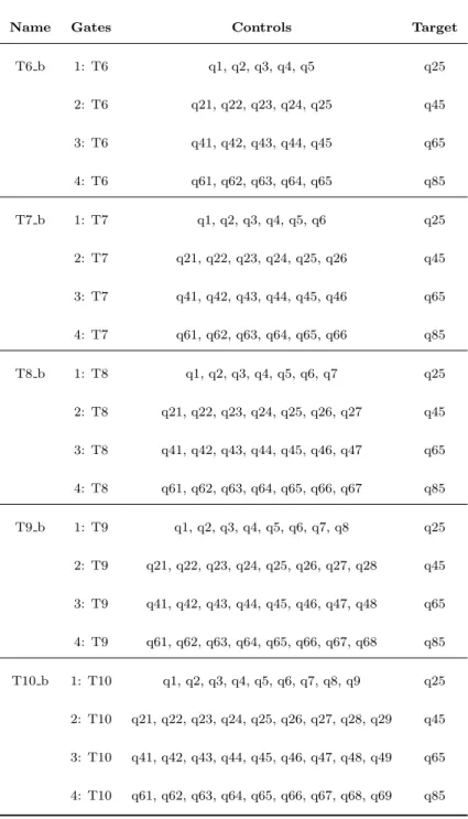
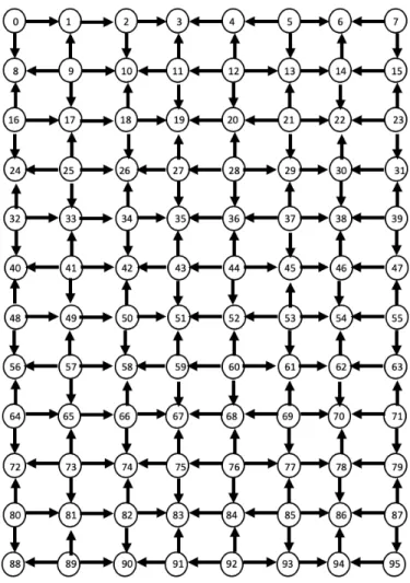
5.2 Proposed 96-qubit machine used for experimentation.. . . 62
5.3 CNOT toCZ transformation.. . . 64
6.1 Comparison of vector spaces for r = 2,3.. . . 72
6.2 Radix-r Chrestenson gate, Cr evolving |φri. . . 75
6.3 Roots of unity in the complex plane for r= 2,3,4, and 5. . . 76
7.1 a) General circuit for radix-r two-qudit partial entanglement generator. b)
Specific example circuit for radix-3 two-qudit partial entanglement generator. 86 7.2 Radix-3 two-qudit maximal entanglement generator implemented with A1,1
and A2,2 that form the composite gate A(1,2),(1,2).. . . 93
7.3 Generalized maximal entanglement circuit for a radix-r qudit pair. . . 96 7.4 Three-qubit GHZ state generator. . . 97 7.5 Radix-3 three-qudit maximal entanglement generator implemented with two
instances of A1,1×A2,2 =A(1,2),(1,2). . . 98
7.6 Generalized structure of circuit needed for radix-r maximal entanglement
amongn qudits where j =n−1 and m=r−1.. . . .100 7.7 Algorithm: Find entangled state generator circuit. . . 101 7.8 Sample output of generator circuit synthesis to prepare √1
3(|003i+|113i+|223i)
from ground state |003i. . . .105
A.1 Signal flow for four-port coupler with input at W.. . . 112 A.2 Macroscopic realization of a four-port coupler. . . 115 A.3 Cross sectional scanning electron microscope image of a four-port coupler
in MQW-InP.. . . .116 A.4 Cross sectional transmission electron micrograph of a four-port coupler
LIST OF TABLES
Table Page
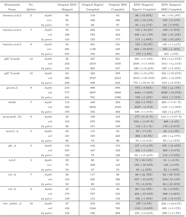
2.1 Common single- and multi-qubit quantum operators . . . 15 3.1 IBM Q device details (* indicates a retired device) (IBM Q team, 2018a,b,c,d,e) 29 3.2 Rigetti device details (* indicates a retired device) (Rigetti Computing, 2019a) 31 3.3 Photonic quantum operators . . . 32 4.1 Gate depth, gate volume, and two-qubit metrics of benchmarks after zdd
mapping, IBM compiling, and Rigetti compiling. Values that decreased whenever ZDD mapping was implemented before compilation have been
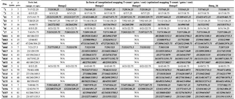
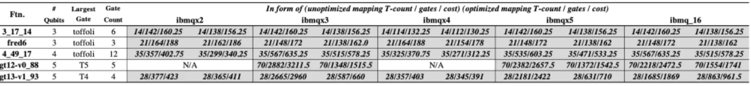
emphasized. . . 51 5.1 Results of compilation using benchmarks from (rev, 2017) mapped to IBM
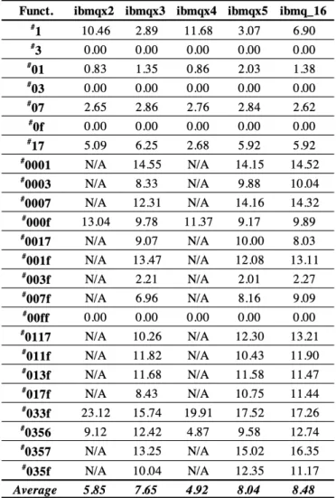
devices.. . . 57 5.2 Percent decrease of (rev, 2017) benchmark cost after optimization.. . . 58 5.3 Results of compilation using benchmarks from (rev) mapped to IBM devices.. . 59 5.4 Percent decrease of (rev) benchmark cost after optimization. . . 60 5.5 96-qubit QC benchmark details.. . . 61 5.6 96-qubit QC benchmark compilation results.. . . 63 5.7 Metrics for (CZ count/cost) after synthesis using benchmarks from (rev,
2017) targeting the Rigetti QCs. . . 66 5.8 Percent decrease in cost from unoptimized to optimized synthesis targeting
the rigetti QCs.. . . 67 7.1 Outputs of radix-3 partial entanglement generator circuit with |03i as
con-trol level . . . 88 7.2 Outputs of radix-3 partial entanglement generator circuit with |13i as
con-trol level . . . 88 7.3 Outputs of radix-3 partial entanglement generator circuit with |23i as
7.4 Outputs of radix-3 maximal entanglement generator circuit with |13i and
|23ias control levels . . . 91
7.5 Outputs of radix-3 maximal entanglement generator circuit with |03i and
|23ias control levels . . . 92
7.6 Outputs of radix-3 maximal entanglement generator circuit with |03i and
|13ias control levels . . . 92
7.7 Outputs of radix-3 three-qudit maximal entanglement generator circuit in
Fig. 7.5. . . 99 7.8 Required generator circuit components for two-qudit maximally entangled
state preparation . . . .103 7.9 Required generator circuit components for multi-qudit maximally entangled
LIST OF ABBREVIATIONS
ALD Atomic Layer Deposition CNOT Controlled-NOT CPU Central Processing Unit CTR Connectivity Tree Reroute CZ Controlled-phase
EPR Einstein, Podolsky, and Rosen ESOP Exclusive Sum of Products FIB Focused Ion Beam
GHZ Greenberger–Horne–Zeilinger HBr Hydrogen Bromide
ICP Inductively Coupled Plasma MQW Multi-quantum Well
NISQ Noisy Intermediate-scale Quantum OAM Orbital Angular Momentum QASM Quantum Assembly Language QC Quantum Computer
QFT Quantum Fourier Transform QIP Quantum Information Processing QKD Quantum Key Distribution
QMDD Quantum Multiple-valued Decision Diagram QPIC Quantum Photonic Integrated Circuits
QPU Quantum Processing Unit QUIL Quantum Instruction Language SDK Software Development Kit
Chapter 1 Introduction
Modern digital circuitry can evaluate complex equations quickly and with precision, al-lowing for rapid rates of data creation and processing. Computers that are modeled with classical switching theory have revolutionized problem solving, but due to their nature, these devices are not ideal for every calculation without large overhead with respect to time or physical resources. The quantum computing model, however, has potential to solve some of these difficult problems with greater efficiency due to a fundamentally different underlying model of computation.
The field of quantum computation is one of great potential. Theoretical work has proven that a quantum computer (QC) can complete tasks such as searching large data sets and simulating quantum behavior at a rate much faster than what is currently possible. In addition, QCs have demonstrated other computing advantages, such as the ability to encode state spaces where the basis dimension is greater than two. Unfortunately, physical QC development is not as advanced as the state of quantum theory and algorithms. Currently, there are many contenders for what will eventually be the standard quantum computing platform or technology.
Because of the variety that exists in quantum implementations and devices, techniques are needed that map quantum circuits, especially those that generate important phenomena such as quantum entanglement, to physical technology platforms that contain varied gate li-braries and qubit layout topologies. Thus, methods for quantum logic synthesis, or hardware compilation, are required.
1.1. Classical Computation and Limitations
The electronic computers that are widely available today are referred to here as classical computers. These devices process information in discrete units of information, modeled as bits, that have a value of either one or zero indicating an asserted or a deasserted state, respectively. Over the last half century, classical computers have consistently improved in their processing power. This advance in technology has helped simplify many complex calcu-lations, such as calculus problems, and has allowed the development of classical algorithms that support the analysis of system reliability (Smith et al., 2017), computer security (Tay-lor et al., 2017), poynomial decomposition (Smith and Thornton, 2019h), and many others. There are, however, still several problems that are impractical to solve on a classical machine due to their spatial or temporal complexities. Additionally, because of the bistable nature of transistors that are standard in electronic technology, the majority of classical computa-tion is based on an implementacomputa-tion of a radix-2 model where the bit takes a single value of B ∈ {0,1}. Due to the very nature of classical computing, the Turing machine model guarantees that theoretical complexities can not be overcome. Examples of problems that are currently difficult for classical computers to solve involve searching large state spaces and factoring numbers (DiVincenzo, 2010). Even if classical computers could continue the trend of increased performance, although the momentum of computational power is slowing due to the inability to continue to scale down the feature size of transistors, complexity issues would still exist because some problems remain intractable. The abilities of classical computers will always exhibit deficits due to the Turing model, leaving many intractable problems unsolved. Therefore, alternative computing methods, such as quantum methods, should be investigated.
1.2. Contribution
The models and rules of quantum computation and quantum information processing (QIP) differ greatly from those that govern classical computation, and these differences have caused quantum device implementation with a variety of new technologies. Many platforms have been developed in parallel, but at the time of writing, one method of quantum comput-ing has not shown to be superior to the rest. Because of the variation that exists between quantum platforms, even between those of the same technology, there must be a way to au-tomatically synthesize technology-independent quantum designs into forms that are capable of physical realization on a QC with specific operating parameters. Additionally, results of synthesis should be verified to confirm that output technology-dependent specifications are logically identical to their original, technology-independent forms. The first contribution of this work to the field of quantum computation is the creation of such a methodology. Quantum technology mapping and optimization for machines with fixed coupling maps and libraries of gates can be performed with an automatic quantum compiler. The development and test of compilation algorithms will be explored in this dissertation. Compilation can be considered in a more general context to be a synthesis tool for QIP circuits in a specific realization technology, and many of these technologies are capable of implementing systems where the radix of computation,r, is greater than two. As a result of this ability, the second contribution of this work is the presentation of architectures for higher-dimensional quantum entanglement.
The contributions above have been included in (Smith and Thornton, 2017, 2018, 2019a,b,c,d,e,f; Smith et al., 2019). Other publications and works completed during my PhD studies include (Smith and Thornton, 2015, 2019g,h; Smith et al., 2017, 2018a,b,c; Taylor et al., 2017).
Chapter 2 Quantum Information
2.1. The Qubit
In classical computation, units of information are stored in strings of bits. Each bit can have a logic value of B ∈ {0,1}. According to switching theory, Boolean logic gates are applied to bit values in order to cause change over time. The mathematical model of Boolean algebra is used to create and manipulate meaningful data from strings of bits, and this information must be represented physically in computing systems such as in the form of voltage or current in a wire or as light in a fiber optic cable. The classical states of 0 and 1 are most frequently realized within electronic devices as either a low or high voltage, respectively, when using positive logic or as a high or low voltage, respectively, when using negative logic.
In QIP, the unit of information is the quantum bit, or qubit. The qubit stores information by holding values such as |0i or |1i which are a set of orthonormal basis states in Dirac notation (Dirac, 1958) that represent the two-dimensional column vectors of
|0i= 1 0 ,|1i= 0 1 . (2.1)
Although similarities between the qubit and the classical bit exist, the qubit may represent an infinite number of states while in a superposition of a set of basis states. For example, the qubit |Ψi may equal either |0i or|1i, or it may take a value that is a linear combination of both basis states in the form of
|Ψi=α|0i+β|1i. (2.2) In Eqn. 2.2, the probability amplitudesα and β are complex numbers,c, that take the form of c =a+bi. Here, i is an imaginary number where i2 = −1. The state of a qubit can be
visualized using the geometry of the Bloch sphere (Bloch, 1946; Nielsen and Chuang, 2010). On the Bloch sphere, pictured in Fig. 2.1, |0i is found at the north pole, ˆz whereas |1i is found at the south pole, −zˆ. The states |0i and |1i are referred to as the computational basis. A qubit may take any value on the surface of the Bloch sphere that represents a linear combination of |0i and |1i.
Figure 2.1. The Bloch sphere
The magnitude of qubit probability amplitudes must sum to unity, thus, the Bloch sphere has a radius of one. In Eqn 2.2, the probability that |Ψi = |0i is equivalent to α∗α = |α|2
and the probability that |Ψi=|1i is β∗β =|β|2 where ∗ indicates a complex conjugate and |α|2 +|β|2 = 1. Once a qubit is measured, it collapses into a basis state and its quantum
2.2. Physical Quantum Implementations
Qubits have been successfully realized in many different mediums. In microscopic real-izations, the size of the particles acting as qubits are on the atomic scale. Because these particles are so small, they exhibit the quantum characteristics needed by the qubit to exist in states of superposition. Of these different particle types, none have proven to be a supe-rior information carrier. Some examples of popular qubit representations within quantum particle systems are photons in optical cavities, photons in microwave cavities, ions in ion traps, spin in electrons, and charge in quantum dots (Nielsen and Chuang, 2010). Qubits can also be realized in larger, mesoscopic systems like with electric charge in solid-state superconducting circuits (Koch et al., 2007).
At the time of writing, quantum technology is in the noisy intermediate-scale quantum (NISQ) era (Preskill, 2018). The QCs available are of modest size, but a significant limiting factor with these devices is the high probability of an accidental measurement of qubit state that causes the system to collapse. This collapse, usually caused by an unintended interaction between a qubit and its environment, is called decoherence (Nielsen and Chuang, 2010). Scientists have observed through experimentation that some quantum systems are more resilient to decoherence than others. For example, the quantum coherence time for a photon within an optical cavity is approximately 10−5 second whereas the quantum coherence time for an indium atom within an ion trap is approximately 10−1 second (Nielsen and Chuang,
2010). More recent implementations with transmons, charge-based qubits used by companies such as IBM and Rigetti, have demonstrated coherence times of approximately 10−4 second (Devoret and Schoelkopf, 2013).
There are two types of qubits in QIP: stationary qubits and “flying” qubits. Stationary qubits are used to perform calculations in fixed locations such as within a integrated cir-cuit. Because stationary qubits are used for computation, they must be implemented with technologies that allow qubits to easily interact with each other. Flying qubits, on the other
hand, are used for the transmission of quantum information. This type of qubit must be implemented with technology resistant to decoherence so the quantum state is stable as it travels.
2.2.1. Transmons
The transmon QC is a popular platform of the NISQ era. The technology was first developed in 2007 at Yale University, and current work with these devices have demon-strated very promising coherence times of around 100 µs (Devoret and Schoelkopf, 2013; Koch et al., 2007). One- and two-qubit quantum state transformations can be executed with high fidelity (Tripathi et al., 2019), and as a result, many companies and research groups, such as IBM and Rigetti, have invested resources to continue to develop transmon technol-ogy. For example, IBM Q includes quantum machines with 5 or more qubits that can be programmed to run user-generated quantum circuits. A discussion of the IBM quantum machines can be found in Section 3.4.1 while information about the Rigetti devices can be found in Section 3.4.2.
Transmons are a physical quantum realization that are categorized as superconducting charge qubits. Superconducting qubits in general use microscopic phenomena within meso-scopic devices, such as electric charge in a circuit for the case of the transmon, to realize quantum information. To better understand how a transmon works, its components must be understood. A Cooper Pair Box, a capacitive shunt, and a transmission line resonator are the main components that comprise a transmon with the Cooper Pair Box being the ele-ment that contains the charge qubit. A Josephson Junction, two superconducting materials separated by a very thin insulator, along with a Cooper pair, two electrons bonded at low energy levels, form the Cooper Pair Box (Bader, 2013).
As indicated by the name “superconducting charge qubit,” electric charge provides the representation of qubit basis states for the transmon. The transmission line resonator on the device provides a means of interacting with the qubit. For example, by applying specific
electric fields to the resonator, a single qubit operation can be performed. Multiple transmon qubits can be coupled together if additional connecting resonators are added, allowing for multi-qubit transformations to occur. More details about the transmon architecture and the available operations can be found in (Bader, 2013; Devoret and Schoelkopf, 2013; Koch et al., 2007).
2.2.2. Photonics
Photonic computing is a promising area that provides some benefits with respect to secu-rity such as resilience to side channel attacks. There have been recent efforts to implement photonic computing using the classical Turing machine model (Singh et al., 2014; Smith and Thornton, 2015), however, the potential of quantum computing and the ability to use photons as qubit state carriers is considered by many in the field to be a more valuable use of photonics.
Photonic implementations could be considered one of the more successful physical quan-tum realizations. Its weaknesses due to the nature of light, however, have prohibited photonic devices from becoming the standard platform for quantum logic. In a photonic QC, qubits are realized with photons. A photonic qubit is characterized by having a long coherence time that can be demonstrated experimentally to travel lengthy distances at room temperature (Myers and Laflamme, 2006). This long coherence time is caused by the photon’s resistance to coupling with other elements in its environment (Kok et al., 2007). While the photonic qubit’s failure to interact with other objects is an advantage in terms of maintaining state, it creates difficulties in situations where qubits must interact in multi-qubit gates such as with the controlled-NOT(CNOT) or controlled-phase (CZ) operations. Single-qubit operations are easily implemented and deterministic with photonics, but multi-qubit gates are currently probabilistic in outcome. For example, the first quantum photonics gate with a control, a conditional phase flip gate, was demonstrated to have a success probability of 161 in 2001 (Knill et al., 2001). These results were improved in 2003 by (O’Brien et al., 2003) when a
photonicCNOTdevice was shown to operate with a success rate of 1
9. Currently, controlled
quantum operations implemented with photonic devices are proven to only have a fidelity of
1
4 in ideal operating conditions (Eisert, 2005).
A physical quantum implementation must have a technique for encoding qubit state. Although other encoding methods exist with quantum photonics, the two main methods for representing the qubit are with photon polarization and location. In the first method, photon polarization acts as the information carrier where two orthogonal polarization angles of light represent a set of quantum basis states. Typically with the polarization-encoded qubit, horizontal polarization represents |0i and vertical polarization represents |1i (Kok et al., 2007). The second method of photonic qubit realization uses what is known as dual-rail representation. Dual-rail representation is a location-based means of representing quantum information. Whenever using location to represent qubit state, it is most common that the top rail represents |0i and the bottom rail represents |1i on quantum circuit diagrams (Kok et al., 2007; Myers and Laflamme, 2006). Converting between polarization-encoded and dual-rail encoded qubits is a relatively easy process that is frequently done in photonic quantum circuitry. To convert between the two forms of photonic qubits, both a polarizing beam splitter and a half wave plate can be used (Myers and Laflamme, 2006; O’Brien et al., 2003). The schematic representing the photonic transformation from a polarization encoding to a location encoding can be seen in Fig. 2.2.
Figure 2.2. Photonic transformation between polarization and dual-rail encoding schemes
Orbital angular momentum (OAM) states of light are also used to encode qubit state (Garc´ıa-Escart´ın and Chamorro-Posada, 2008).
Choosing a qubit encoding scheme for a photonic quantum implementation depends on the qubit’s task. For example, since fewer communication lines are needed for the polarization-encoded qubit, this representation may be more suitable for long-haul qubit transmissions. Whenever photonic quantum computations are performed, however, dual-rail representation is most frequently used. Additionally, dual-rail encoding is easier to imple-ment on quantum photonic integrated circuits (QPICs). More information about photonic quantum operators for both polarization and location encoding methods can be found in Section 3.4.3.
2.3. The Superposition Principle
In Section 2.1, the concept of superposition for a single qubit was introduced. Because of superposition, if|Ψiand|Φiare two quantum basis states for a qubit, any linear combination of these two states, α|Ψi+β|Φi is also a valid state of the system where |α|2 +|β|2 = 1.
The superposition principle, however, is one that does not only pertain to a single qubit. Quantum networks composed of multiple qubits can be in states of superposition as well. For example, if there are two quantum systems, and these two systems have their quantum state held in the vectors |xi = α1|Ψi+β1|Φi =
α1 β1 and |yi = α2|Ψi+β2|Φi = α2 β2 ,
respectively. If these two systems were to be combined, the vector |xyi would be formed by the tensor product of two original state vectors:
|xyi=|xi |yi=|xi ⊗ |yi= α1 β1 ⊗ α2 β2 = α1α2 α1β2 β1α2 β1β2
Due to the superposition principle, any linear function of the possible basis states of the multi-qubit system is also a valid state, as long as the inner product, or the dot product, of the vector formed from the qubits’ combined state equals unity.
2.4. The Wavefunction and Quantum Computing
Quantum mechanics is commonly viewed under the perspective of the Schr¨odinger pic-ture. When looking through this lens, state vectors evolve in time and operators are constant with respect to time. In other words, operators act on a wavefunction, Ψ, a mathematical description of the quantum points of interest of a system, causing change. The wavefunction includes complex-valued amplitudes, and the probabilities for the possible outcomes from measurement of the system can be derived from solving|Ψ|2 = Ψ∗Ψ (Griffiths, 1995). Upon
measurement, the wavefunction collapses into a basis state of the system. The wavefunction is a solution of the time- and position-dependent Schr¨odinger equation
i~∂Ψ(x, t)
∂t = ˆHΨ(x, t). (2.3)
In the equation above,i=√−1, and~is the reduced Planck constant. ˆH is the Hamiltonian operator, ˆ H =− ~ 2 2m ∂2 ∂x2 +V(x), (2.4)
that represents the total energy for a system where where m represents mass and V(x) represent potential as a function of position. The differential equation of Eqn. 2.3 can be solved to derive an expression for the wavefunction. To begin, the right side of the Eqn. 2.3 will be expanded using Eqn. 2.4 to form
i~∂Ψ(x, t) ∂t =− ~2 2m ∂2Ψ(x, t) ∂x2 +V(x)Ψ(x, t). (2.5)
A function that describes how Ψ(x,0) evolves into Ψ(x, t) is desired, but this is difficult to find while the Schr¨odinger equation contains partial differential equations. To put Eqn. 2.5 into a simpler form, a separation of variables technique will be applied to find a solution in the form of Ψ(x, t) = F(t)Ψ(x) where the time and position components of Ψ(x, t) are separated into two different equations, respectively, that intersect under multiplication. The
reason why Ψ(x, t) is written as two functions rather than one is because it allows difficult partial derivatives to become total derivatives. Writing Eqn. 2.5 with Ψ(x, t) = F(t)Ψ(x) gives i~Ψ(x)dF(t) dt = −~ 2 2m d2Ψ(x)F(t) dx2 +V(x)Ψ(x)F(t) , i~Ψ(x)dF(t) dt =F(t) − ~ 2 2m d2Ψ(x) dx2 +V(x)Ψ(x) ,
which can be reduced using Eqn. 2.4 to
i~Ψ(x)dF(t)
dt =F(t) ˆHΨ(x).
So that time- and position-dependent functions are grouped. Next, both sides of the equation will be divided byF(t)Ψ(x) to give
i~ 1 F(t) dF(t) dt = 1 Ψ(x) ˆ HΨ(x) =E. (2.6)
Note how Eqn. 2.6 has the time- and position-dependent parts separated by the equals sign. Since changes to either x or t would cause only the right or left side of the equation to change, respectively, they need to be related by a term that is not a function of either variable. This term is a constant, E, that allows states of definite energy, or an eigenvectors of the Hamiltonian, to be expressed. Two new equations surface from the manipulation of Eqn. 2.6: i~dF(t) dt =EF(t), (2.7) and ˆ HΨ(x) =EΨ(x). (2.8)
Eqn. 2.7 is time-dependent and Eqn. 2.8 is time-independent and is instead dependent on position. Now the wavefunction can be solved while keeping the value forE in both Eqn. 2.7 and Eqn. 2.8 equal. Solving the differential equation in Eqn. 2.7 allows
i~dF(t)
dt =EF(t),
to become
F(t) = F(0)e−iEt/~.
Now that the time-dependent Eqn. 2.7 has been solved, the variables can be recombined to create the wavefunction
Ψ(x, t) =F(t)Ψ(t) =F(0)e−iEt/~Ψ
E(x), thus,
ΨE(x, t) = e−iEt/~ΨE(x, t= 0). (2.9) The subscript E is used to denote that Ψ(x) is associated with the same state of definite energy as that of F(t).
In quantum computing, the state of the wavefunction Ψ is written using dirac notation and is embodied by the qubit. For instance, the qubit |Ψi can be in a state of either |0i
or |1i, or in a superposition of both simultaneously. After measurement, it collapses into one of the basis states. The qubit is transformed by quantum gates that are represented collectively by Usuch that
U=e−iEt/~ = u00 u01 u10 u11 . (2.10)
U is a unitary operator. When U is substituted into Eqn. 2.9, the following form of the wavefunction,
|ΨE(x, t)i=U|ΨE(x, t= 0)i, (2.11) results. In Eqn. 2.11, U allows |ΨE(x, t= 0)i to transform into |ΨE(x, t)i over time.
2.5. Quantum Operations
Quantum operators transform qubit state to implement quantum computation. If a quantum algorithm were to be thought of as a circuit, the quantum operators would be the gates. These operators are represented by a unique transfer function matrix of size 2n×2n where n is the number of qubits that the operation transforms. The transformation matrix for a quantum operator, U, is always unitary, so the following characteristics are observed:
• U†U= UU† =In,
• U−1 = U†, • Rank(U) = n,
• |U| = 1.
In the identities above, the symbol † indicates a complex-conjugate transpose. Gate trans-formations can take place on single or multiple qubits. Some of the most common one- and two-qubit operations are included in Table 2.1.
The transformations described in Table 2.1 are frequently used quantum operations, and controlled variations of these gates can also be defined. For example, the CNOToperation is the controlled Pauli-X, or controlled NOT, operation where a control qubit determines the enable operation on a target qubit. Additional controls can be added onto the CNOT. The transformation matrix and symbol for the Toffoli operation, an operator that acts as a controlled-CNOT, can be seen in Table. 2.1. Adding more control qubits onto a Toffoli gate results in ann-qubit generalized Toffoli wherem=n−1 qubits act as controls and the
Table 2.1. Common single- and multi-qubit quantum operators
Operator Symbol Transfer Matrix
Pauli-X (X) h0 1 1 0 i Pauli-Y (Y) h0 −i i 0 i Pauli-Z (Z) h1 0 0 −1 i Hadamard (H) √1 2 h 1 1 1 −1 i Phase (S) h1 0 0 i i π/8 (T) h 1 0 0 eiπ/4 i CNOT 1 0 0 0 0 1 0 0 0 0 0 1 0 0 1 0 CZ 1 0 0 0 0 1 0 0 0 0 1 0 0 0 0 −1 SWAP 1 0 0 0 0 0 1 0 0 1 0 0 0 0 0 1 Toffoli 1 0 0 0 0 0 0 0 0 1 0 0 0 0 0 0 0 0 1 0 0 0 0 0 0 0 0 1 0 0 0 0 0 0 0 0 1 0 0 0 0 0 0 0 0 1 0 0 0 0 0 0 0 0 0 1 0 0 0 0 0 0 1 0
Quantum operators are combined to form quantum circuits, and quantum circuits can be described in a variety of ways. Some of the most popular techniques include drawing the circuits as graphs, like the one seen in Fig. 2.3, or describing them as a netlist with Quantum Assembly Language (QASM) or Quantum Instruction Language (Quil).
Understanding how information is transformed in a quantum circuit requires some knowl-edge of linear algebra and tensor products. As seen in Table. 2.1, quantum operators are represented by transformation matrices. To determine the resulting quantum state, |Ψouti, after gate transformation, U, the calculation
|Ψouti=U|Ψini (2.12)
must be completed. To determine |Ψini, the input qubit values are combined via tensor product. Consider the quantum circuit pictured in Fig. 2.3. In this circuit, two qubits, |ai
and|bi, are each represented by a single horizontal line, but these horizontal lines should not be confused with conductors like those in electrical circuit schematics. Reading from left to right on the graph, qubit state evolves as time progresses and they pass though theCNOT gate. Together at the input they form the value of |Ψini and
|Ψini=|aini ⊗ |bini=|1i ⊗ |0i= 0 1 ⊗ 1 0 = 0 0 1 0 =|10i.
Determining |Ψouti requires Eqn. 2.12 to be used, and in this case, CNOT will take the place of generalized transformation matrix U to generate
|Ψouti=U|Ψini=CNOT|10i= 1 0 0 0 0 1 0 0 0 0 0 1 0 0 1 0 0 0 1 0 = 0 0 0 1 =|11i .
Figure 2.3. Quantum circuit example 1
Quantum operators are not limited to radix-2, or base-2, operations. Higher-order gates act on quantum digits or “qudits” that are characterized by three or more basis states. An example radix-4 Chrestenson gate can be found in (Smith et al., 2018a,b) and in Ap-pendix A. Methods and operators for generating higher-radix quantum entanglement are found in (Smith and Thornton, 2019a,c) and within Chapter 6 and Chapter 7.
2.6. Requirements for Quantum Computation
Quantum computation holds the key to unlocking the mystery of nature as QCs are the ideal devices for the simulation of physics (Feynman, 1982). Performing quantum compu-tations, however, requires more than simply realizing a qubit in a physical medium. For example, while it is important for a system to demonstrate quantum characteristics to hold qubits, these qubits must be able to evolve and interact with each other in order to represent computation. In (Deutsch, 1985), a work that many scientists accept as the fundamental model for quantum computation, the requirements for a quantum computer are described in detail. According to this paper, a grouping of n qubits that are successfully able to act as a
quantum computer must demonstrate the following:
• Qubits must be initialized to a known state, such as |0i or |1i.
• Qubits must be measurable, causing their collapse into a basis state.
• A qubit (or set of qubits) has the ability to evolve through a universal quantum gate or set of gates, U, in a series that represents a unitary transformation (i.e. operations are reversible becauseUU†=U† U=I).
• Qubits maintain their current quantum state if the aforementioned actions do not occur.
The requirements above list the basic necessities for the evaluation of a quantum algorithm. They describe a system where the outputs of the circuitry are dependent only on the current inputs, or the original qubits that were initialized to a known state. If viewed from a classical computing perspective, the requirements outlined in (Deutsch, 1985) allow us to realize combinational quantum logic circuits where the output is a function of the current circuit input only. These theoretical concepts for quantum computing have been expanded since their original introduction in 1985.
In (DiVincenzo, 2010), the essential operational characteristics for a quantum computer are described in greater detail along with the requirements for communicating in quan-tum networks. In addition to the above necessities for quanquan-tum algorithm execution from (Deutsch, 1985), (DiVincenzo, 2010) states that a practical quantum computer will need to be built using technology that is scalable and is capable of long coherence times to main-tain qubit state during computation. For quantum computation between machines, qubits must be transmitted in a controlled manner, and those transmitted qubits, known as “flying qubits,” must interact with stationary qubits in order to produce meaningful information (DiVincenzo, 2010).
2.7. Entanglement
Entanglement is one of the most significant quantum phenomena. It describes how two or more qubits can interact in such a way where they become a composite system that is no longer separable. In other words, none of the member qubits can be described independently from the qubit group once the group is in an entangled state. From a mathematical point of view, if |Ψi is an entangled quantum state, it cannot be expressed as a product |xi ⊗ |yi
of its component systems. The following four states are examples of two-qubit entangled states: |β00i= |00i+|11i √ 2 , (2.13) |β01i= |01i+|10i √ 2 , (2.14) |β10i= |00i − |11i √ 2 , (2.15) |β11i= |01i − |10i √ 2 . (2.16)
The states listed in the equations above are known as the Bell states. In some texts, they are also referred to as EPR states, or pairs, after Einstein, Podolsky, and Rosen and their groundbreaking paper (Einstein et al., 1935). The Bell states represent how two qubits may be maximally entangled, or each of the possible outcomes of an observation are equally likely. A Hadamard gate followed by aCNOTgate can be used to create Bell state entanglement. The Bell state generating circuit is pictured in Fig. 2.4. Entanglement between two qubits is not limited to just the Bell states, however. Other arbitrary entangled pairs are possible where the probability amplitudes are unequal.
One of the significant properties of an entangled qubit pair is that knowledge of a single qubit in the set gives insight to the rest of the member qubits. For example, consider a
Figure 2.4. Bell state generator
two-qubit system in the Bell state of |β00i. Before measurement, the system has an equal
probability of being in either state |00ior state |11i, respectively. During computation, the first qubit is measured, and it collapses into a basis state. If the first qubit is measured to be a|0i, the second qubit must also be|0ibecause the two qubits in the system were entangled. Likewise, if the first qubit is measured to be a |1i, the second qubit must also be|1i.
Quantum entanglement is an important phenomenon that is a critical component of most quantum computation and communications algorithms. The ability to experimen-tally demonstrate entanglement is significant because this phenomenon enables quantum computing algorithms that exhibit a computational advantage as compared to their classical counterparts. Another very important application of entanglement is that it allows for the im-plementation of ultra-secure quantum communications protocols. For example, although the original BB84 quantum key distribution (QKD) protocol only relies on superposition (Ben-nett Ch and Brassard, 1984), entanglement is necessary for many BB84 derivatives (Ekert, 1991; Enzer et al., 2002). Additionally, quantum factoring of composite prime numbers (Shor, 1994), quantum radar (Lanzagorta, 2011), quantum teleportation (Bennett et al., 1993), and many other applications depend upon and exploit the properties of entanglement in their implementation. The entire concept of many QIS systems such as teleportation, quantum communication channels, and others are based on the property of entanglement. Recently, the well-known recent Chinese experiments based upon their Micius satellite demonstrated that a quantum channel could be created between the earth and space. The Micius
exper-iments utilized quantum entanglement generators as a key function (Yin et al., 2017) for their impenetrable communication network.
Chapter 3
Quantum Logic Synthesis Considerations
3.1. No-Cloning Theorem
Another unique characteristic quantum computation that further distinguishes it from the classical computation model is the inability copy information. This property is especially apparent whenever qubits are in a superimposed state. A classical bit encoded as a voltage level can ideally fan out onto multiple branches as connections are added in parallel. Due to the no-cloning theorem, a similar action cannot be performed on a qubit that results in the creation of two qubits with identical value (Nielsen and Chuang, 2010).
Figure 3.1. Proposed qubit copying gate, G
The no-cloning theorem can be proven using a contradiction. Assume that there exists a generalized cloning gate, G, that transforms any steady state, such as |0i, into a copy of a qubit, |Ψi. The transformation G is represented by a unitary transformation matrix as is required for quantum gates. A block diagram describing the function of the proposed gate G can be seen in Fig. 3.1. With G, two orthogonal quantum basis states are cloned, G(|Ψ0i) = |ΨΨi and G(|Φ0i) =|ΦΦi. Attempts to copy a state that is in a superposition
of these basis states, however, is not as successful. The qubit |βi = √1
2(|Ψi+|Φi) will be
the example state that will undergo the cloning transform: Anticipated cloned value of|ββi:
|ββi= √1 2(|Ψi+|Φi)⊗ 1 √ 2(|Ψi+|Φi) = 1 2[|ΨΨi+|ΨΦi+|ΦΨi+|ΦΦi] Actual value of|ββi after applying cloning transform, G:
G(|β0i) =G 1 √ 2(|Ψi+|Φi)|0i = √1 2[G(|Ψ0i) +G(|Φ0i)] = 1 √ 2[|ΨΨi+|ΦΦi] The anticipated cloned value of |ββi using G and the actual value are unequal. This con-tradiction proves the no-cloning theorem since it shows that Gcannot exist.
The limitations of the no-cloning theorem on the qubit have severe implications in terms of how quantum algorithms store information. Because of the inability to copy a qubit, quan-tum memory will differ greatly from a classical memory. An example of a proposed method to implement quantum storage using ring oscillator structures can be found in (Smith et al., 2018c). While a classical bit can theoretically be read from memory as many times as nec-essary while it occupies a memory address, stored qubits are available for one use only as measurement causes superposition to collapse into a basis state. It is reasonable to conclude that to agree with the no-cloning theorem, any sort of space that once held quantum infor-mation will be invalid after a qubit is retrieved from storage for use if no sort of regeneration of the qubit occurs. The no-cloning theorem is just one of many examples of qubit proper-ties that change the way engineers must think about information storage while developing quantum designs and performing compilation procedures. Quantum information is highly sensitive and cannot be copied, and this characteristic must be taken into consideration whenever transforming a quantum algorithm into a QC executable.
3.2. Reversible Logic
Reversible logic is a type of logic where information can travel bidirectionally without loss. In a reversible circuit, a combination of inputs is sent through a function,fREV(x1, x2, ..., xn),
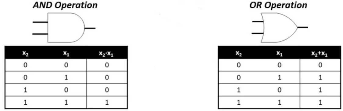
to produce a set of outputs, [y1, y2, ..., ym]. If these outputs are sent back through the inverse of the function, fREV−1 (y1, y2, ..., ym), the original inputs, [x1, x2, ..., xn], are generated. Boolean operations such as the AND and OR operations are not inherently reversible. The truth tables and symbols for these operations can be found in Fig. 3.2. It is apparent while examining these Boolean functions that the outputs are easily derived from the inputs, but information cannot travel in the reverse direction with the same clarity. For example, the output for the AND function is simple to derive with a set of inputs. The function isx2·x1 = 0
whenever the input variables are x2x1 = 00,01,10 and is x2 ·x1 = 1 whenever x2x1 = 11.
Since there are three possible combinations of inputs that allow the AND operation to equal zero, however, there is no way to know with certainty what combination is present at the input of the gate if only the output of zero is known. This is caused by an irretrievable loss of information that occurs as soon as the input signals produce an output from the Boolean logic gate. The loss of information is directly related to total energy dissipated by the circuit according to Landauer’s principle where each bit of erased data costs at minimum
kTln(2) Joules in energy dissipation (Landauer, 1961). Therefore, as a computer loses less information during calculations, it improves in efficiency.
According to the work in (Bennett, 1973), any irreversible function can be made reversible without drastically increasing its spatial and temporal complexity during computation. A motivating reason to convert functions into a reversible form would be to minimize the amount of required power during operation if a physically reversible medium is available. To make an arbitrary switching function a reversible function, it must be transformed into a bijection in which it displays the characteristics of being one-to-one and onto (Fazel et al., 2007). When a function is one-to-one, each element in the codomain, or the target set of the
function, is the image of at most one element in the domain, or the set of input argument values. When a function is onto, each element in the codomain is the image of at least one element in the domain.
Figure 3.2. Boolean AND and OR operation symbols and truth tables
Although reversible logic was a concept that existed before quantum logic was popular-ized, reversible forms of classical circuits could be thought of as a subset of quantum circuits as all quantum circuits are inherently reversible. This is caused by unitary operators where U† = U−1. Because of this property, a quantum transformation followed by its adjoint on
a vector of qubits results in the original quantum state since UU† = I. For example, since CNOTis self-adjoint where CNOT=CNOT−1, so
CNOT2|10i= 1 0 0 0 0 1 0 0 0 0 0 1 0 0 1 0 1 0 0 0 0 1 0 0 0 0 0 1 0 0 1 0 0 0 1 0 = 1 0 0 0 0 1 0 0 0 0 1 0 0 0 0 1 0 0 1 0 = 0 0 1 0 =|10i.
Algorithms exist that transform Boolean logic functions into a reversible form. This process requires the addition of ancilla input values and garbage output values since the amount of inputs and outputs must be equal in a reversible logic function. Once Boolean functions are reversible, they may be compiled into circuits that are executable on a quantum
machine. An example of a reversible logic generator is the work discussed in (Fazel et al., 2007). This algorithm inputs a Boolean logic function in its exclusive sum of products, ESOP, form and converts it to a reversible Toffoli cascade. Another example of a reversible logic synthesis tool is RevKit (Soeken et al., 2012). This program includes ESOP transformation algorithms based on the work first described in (Fazel et al., 2007) as well as decision diagram based reversible logic synthesis techniques. Recent work has resulted in a methods that transform irreversible switching functions into reversible forms with a minimal number of ancillary information carriers (Gabrielson and Thornton, 2018a,b).
3.3. Gate Libraries and Coupling Constraints
There are various architectures for qubit representation currently competing to become the standardized quantum computing platform. This variety between machines, even be-tween those using the same underlying technology, causes conflicts during the circuit design process. For example, several different transmon-based QCs have been developed by the companies IBM and Rigetti. Although these implementations represent quantum informa-tion with transmon technology, differences in architecture topology and gate libraries create compatibility issues which, in many cases, prohibit the use of designs originally mapped for one QC to properly run on another device. This challenge motivates the development of techniques to automatically decompose, map, and optimize quantum circuits to forms that are technologically dependent and physically executable.
Quantum devices have a small set of gates, often ones that are limited to single- and two-qubit transformations, that are physically executable. Because quantum algorithms are usually specified using high-level, multi-qubit operations, they must be simplified into primitive operations that are available in a gate library if the functions are to be physically realized on a real machine. Additionally, although current QCs contain a modest number of physical qubits, connections between qubits on these devices are sparse. Because of nearest neighbor coupling constraints, not all qubit combinations are going to be available
for multi-qubit operations. Therefore, special techniques are required to map the decomposed operations of a generalized quantum circuit so that multi-qubit operations are executable on an architecture.
3.4. Current Physical Quantum Technology
3.4.1. IBM Q
IBM has developed QCs based on solid-state, superconducting circuit technology, and quantum information is realized with the charge-based transmon qubit (Chow et al., 2014a; C´orcoles et al., 2015; Takita et al., 2017). The company has developed real quantum machines and a quantum simulator that the public can access and perform experiments on. The Python software development kit (SDK) Qiskit is used to implement QIP with their platform.
Circuits targeted for the IBM machines must consist of single-qubit operators that are within the gate set of Rz(φ), Rx(θ), Ry(γ). This includes the common transformations of
Identity, Pauli-X, Pauli-Y, Pauli-Z, Hadamard (H), Phase (S), Phase† (S†), π/8 (T),π/8† (T†), phase rotation (φ angle on Bloch sphere), and amplitude rotation (θ angle on Bloch sphere). The CNOT gate is the only available two-qubit gate on the IBM QCs, and its implementation is restricted to a specific coupling map that is set by the connectivity of the transmons on the device. The coupling map prevents arbitrary CNOT placement. Gener-alized quantum circuits must be redesigned so that CNOT gates are mapped to connected qubits. The coupling maps for the public IBM devices can be represented as dictionaries wheredevice ={a0 : [b0], a1 : [b1], . . . , an−1 : [bn−1]}. In these dictionaries, the keywords, ai,
are qubits that can act as CNOTcontrols and the paired list, bi, indicate the qubit(s) that the CNOT control can target (IBM Q team, 2018a,b,c,d,e):
• ibmqx2 = {0:[1,2], 1:[2], 3:[2,4], 4:[2]}
12:[5,11,13], 13:[4,14], 15:[0,14]} • ibmqx4 = {1:[0], 2:[0,1], 3:[2,4] 4:[2]} • ibmqx5={1:[0,2], 2:[3], 3:[4,14], 5:[4], 6:[5,7,11], 7:[10], 8:[7], 9:[8,10], 11:[10], 12:[5,11,13], 13:[4,14], 15:[0,2,14]} • ibmq 16 ={1:[0,2], 2:[3], 4:[3,10], 5:[4,6,9], 6:[8], 7:[8], 9:[8,10], 11:[3,10,12], 12:[2], 13:[1,12]}
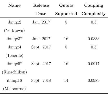
The IBM quantum simulator includes additional gates and qubits that are unrestricted by a coupling map. Information about select IBM machines can be found in Table 3.1. This table contains information about QC name, date of release, capacity, and coupling complexity.
QCs differ in size and layout, and these variations determine the extent that a general circuit must be modified for realization on a particular machine. To give designers better insight to the available qubit connections within a machine, a metric referred to as the “coupling complexity” was devised. The term complexity was chosen to describe the amount of topological interconnects between qubits on a QC. In Table 3.1, coupling complexity is the ratio of the number of allowable CNOT couplings found in the coupling map to the total number of two-qubit permutations for an IBM quantum machine calculated as
IBM coup. complex. = total available couplingsq!
(q−2)!
(3.1) whereq is the number of physical qubits on the machine. For example, the ibmqx2 machine has 6 couplings on the coupling map and a total of 20 two-qubit permutations. Therefore,
ibmqx2 coup. complex. = 6 available couplings
20 total coupling permutations = 0.3.
A coupling complexity close to one indicates that a high percentage of a quantum machine’s qubits are coupled for arbitrary two-qubit CNOToperations. A coupling complexity close to zero indicates a low percentage of coupled qubits.
Table 3.1. IBM Q device details (* indicates a retired device) (IBM Q team, 2018a,b,c,d,e)
Name Release Qubits Coupling Date Supported Complexity
ibmqx2 Jan. 2017 5 0.3 (Yorktown) ibmqx3* June 2017 16 0.0833 ibmqx4 Sept. 2017 5 0.3 (Tenerife) ibmqx5* Sept. 2017 16 0.0917 (Rueschlikon) ibmq 16 Sept. 2018 14 0.0989 (Melbourne) 3.4.2. Rigetti
Rigetti has developed three solid-state-circuit-based QCs named Agave, Aspen, and Acorn (Didier et al., 2018; Otterbach et al., 2017; Reagor et al., 2018). The Python library PyQuil as well as a software development kit (SDK) Forest are used for writing quantum al-gorithms, interacting with the quantum devices, and simulating quantum computing (Rigetti Computing, 2019b). To specify an algorithm for the Rigetti QCs, quantum operators must be specified in quantum instruction language, or Quil (Smith et al., 2016). Although Quil allows for the specification of algorithms using many of the standard quantum gates, for al-gorithm to be executable on a real quantum processing unit (QPU), a native gate set must be used. This set includes Rz(φ) rotations, Rx(θ) rotations rotations that are integer-multiples
of π/2, and CZ (Rigetti Computing, 2019b).
Not every qubit pair can couple on a QPU, and this severely limits the total number of ex-ecutable multi-qubit operations. The Rigetti devices demonstrate this operational constraint
because the only available two-qubit gate, CZ, may only be implemented on adjacent qubits that are connected. Therefore, the device topology prevents the execution of arbitrary CZ operations in an algorithm. The device topology for the Rigetti QPUs can be represented as dictionaries where device = {a0 : [b0], a1 : [b1], . . . , an−1 : [bn−1]}. In these dictionaries, the
keywords, ai, are qubits that can act as CZ controls and the paired list, bi, indicates which qubit(s) that the CZ control can target (Rigetti Computing, 2019a):
• Agave ={ 0:[1,7], 1:[0,2], 2:[1,3], 3:[2,4], 4:[3,5], 5:[4,6],6:[5,7], 7:[0,6] } • Aspen ={ 0:[1,7], 1:[0,2,16], 2:[1,3,15], 3:[2,4], 4:[3,5], 5:[4,6], 6:[5,7], 7:[0,6], 10:[11,17], 11:[10,12], 12:[11,13], 13:[12,14], 14:[13,15], 15:[2,14,16], 16:[1,15,17], 17:[10,16] } • Acorn = {0:[5,6], 1:[6,7], 2:[7,8], 4:[9], 5:[0,10], 6:[0,1,11], 7:[1,2,12], 8:[2,13], 9:[4,14], 10:[5,15,16], 11:[6,16,17], 12:[7,17,18], 13:[8,18,19], 14:[9,19], 15:[10], 16:[10,11], 17:[11,12], 18:[12,13], 19:[13,14] }
Information about the Rigetti machines that details QC name, date of release, capacity, and coupling complexity can be found in Table 3.2. An interesting observation is that the CZ gate is bidirectional in the sense that the transformation matrix is equivalent if the control and target qubits are interchanged. Because of the bidirectional nature of the CZ gate, Rigetti coupling complexity is calculated with combinations rather than permutations as
Rigetti coup. complex. = total available couplingsq!
2(q−2)!
. (3.2)
3.4.3. Quantum with Photonic Devices
Photons are a great medium for representing qubit state. They are stable particles in the sense that they do not couple easily with their environment. Additionally, photons are not spatially stationary particles. Since they resist decoherence, photons retain quantum information for long periods of time at room temperature. This property makes them suitable
Table 3.2. Rigetti device details (* indicates a retired device) (Rigetti Computing, 2019a)
Name Release Qubits Coupling Date Supported Complexity
Aspen Nov. 2018 16 0.15
Agave* June 2018 8 0.2857
Acorn* Dec. 2017 19 0.1345
as flying qubits. The photon’s resistance to decoherence, however, causes the implementation of multi-qubit gates to be difficult. Because photons fail to easily interact with each other, multi-qubit gates act in a probabilistic rather than in a deterministic manner.
A popular methodology for implementing a photonic universal quantum computer is with the KLM protocol (Knill et al., 2001). This protocol uses linear photonics which are devices that transform light in a linear fashion. Examples of linear photonic devices are lenses, mirrors, wave plates, phase shifters and beam splitters. Examples of nonlinear photonic devices include materials that demonstrate the higher-ordered Kerr effect where refractive index of a material is a function of the applied electric field. Because linear devices are used, multi-qubit operations have probabilistic outputs. If a KLM protocol quantum computer is used, it is critical to incorporate error detection and correction in order to repair data after multi-qubit interactions occur. Photonic qubits can either be polarization encoded or dual-rail encoded with the KLM protocol. Table 3.3 has descriptions of photonic quantum operators that operate according to KLM protocol. These components are constructed using elements such as wave plates, beam splitters, and phase shifters. This table of photonic operator implementations, however, is not all inclusive; alternative realizations for photonic gates also exist. Table 3.3 was formed using the information from references (Knill et al., 2001; Knill, 2002; Lemr et al., 2015; Myers and Laflamme, 2006; Nielsen and Chuang, 2010; O’Brien et al., 2003).
Table 3.3. Photonic quantum operators
Operator Symbol Polarization-encoded Implementation Dual-rail Implementation Z-axis Rotation (Phase Shift) 𝐑𝐳(𝛟) = [𝒆−𝒊𝝓/𝟐 𝟎 𝟎 𝒆𝒊𝝓/𝟐] Deterministic Pauli-Z 𝒁 = [𝟏 𝟎 𝟎 −𝟏] Deterministic Phase (S) 𝑺 = [𝟏 𝟎 𝟎 𝒊] Deterministic π/8 (T) 𝑻 = [𝟏 𝟎 𝟎 𝒆𝒊𝝅/𝟒] Deterministic Pauli-Y 𝒀 = [𝟎 −𝒊 𝒊 𝟎] Deterministic NOT (Pauli-X) 𝑿 = [𝟎 𝟏 𝟏 𝟎] Deterministic Hadamard 𝑯 = 𝟏 √𝟐[ 𝟏 𝟏 𝟏 −𝟏] Deterministic √𝑵𝑶𝑻 𝑽 =𝟏 𝟐[ 𝟏 + 𝒊 𝟏 − 𝒊 𝟏 − 𝒊 𝟏 + 𝒊] 𝑽†= 𝟏 𝟐[ 𝟏 − 𝒊 𝟏 + 𝒊 𝟏 + 𝒊 𝟏 − 𝒊] Deterministic Measurement 𝑴|0⟩= [𝟏 𝟎] 𝑴|𝟏⟩= [𝟎 𝟏] Deterministic CNOT CNOT= [ 𝟏 𝟎 𝟎 𝟏 𝟎 𝟎 𝟎 𝟎 𝟎 𝟎 𝟎 𝟎 𝟎 𝟏 𝟏 𝟎 ] Probabilistic, P = 1/9 Controlled-Z CZ= [ 𝟏 𝟎 𝟎 𝟏 𝟎 𝟎 𝟎 𝟎 𝟎 𝟎 𝟎 𝟎 𝟏 𝟎 𝟎 −𝟏 ] Probabilistic, P = 1/16 Tunable Controlled Phase Gate 𝑪𝑹𝒛(𝝓)= [ 𝟏 𝟎 𝟎 𝟏 𝟎 𝟎 𝟎 𝟎 𝟎 𝟎 𝟎 𝟎 𝟏 𝟎 𝟎 𝒆𝒊𝝓 ] Probabilistic, P = 1/48 Implementation Conversion 32
3.5. Quantum Cost
Whenever engineers think of cost, usually measures for reducing power consumption, delay, and area of a circuit come to mind. Classical computation has advanced to the point where certain parameters can be tuned during the design process to optimize one or more of these metrics. It is often the case, however, that all three of these circuit characteristics cannot be improved simultaneously because measures made to improve one property can negatively impact another.
Quantum engineers are still working towards building a reliable and scalable QC during the NISQ era, so designers have less freedom with implementation parameters. Since the main goal for researchers is to allow quantum algorithms to run on physical devices, the reduction of instances where qubit state could decohere is of high importance. With current implementations, quantum state eventually decoheres after time, but its liklihood of deco-herence increases as a qubit undergoes more transformations. Additionally, circuit depth and gate volume is a concern as devices have limited execution times and must be period-ically recalibrated. Since each transformation requires a finite amount of time, whenever thinking about reducing cost for a quantum circuit, reducing the total number of operations performed on a qubit, especially those that implement multi-qubit operations, is of high priority. All arbitraryn-qubit gates are capible of being decomposed into the set of all single qubit gates as well as the CNOT or CZ gate (Barenco et al., 1995). Because of this, one can conclude that an important measurement of cost for quantum circuit is the total number of multi-qubit operations it requires.
Cost functions need to be tunable during quantum logic synthesis and compilation so that key circuit features can be optimized. It is expected that each particular technologically-dependent quantum cell library will be characterized and annotated with custom cost func-tions for use during synthesis depending on if metrics such as qubit fidelity, operator fidelity, or decoherence times are of focus. In this work, the quantum cost function for the IBM
back-end was defined as
qcost = 0.5×t+ 0.25×c+a (3.3) however optimization methods allow for any cost function to be used.
In Eqn. 3.3, t is the count of all T and T† gates, c is the count of CNOT gates, and a
is the total gate count, or gate volume, for a circuit. T gates are given an additional cost of 0.5 as compared to all other single qubit gates because of the operator’s poor fidelity as compared to other single qubit operators in fault tolerant quantum implementations (Amy et al., 2014). CNOTgates are given a cost that is 0.25 more than single qubit gates, with the exception of T, because two-qubit operations for the transmon are characterized by higher error rates as compared to the other single qubit operations (Chow et al., 2014b). The IBM cost function was selected based upon what is commonly seen in the literature: fewer gates usually leads to smaller circuits with a lower probability for decoherence and fewer T gates improves reliability and results in greater fault-tolerance. A larger quantum cost indicates a higher likelihood of qubit decoherence and decreased fault tolerance. Quantum cost for a design is minimized by quantum logic design automation tools during the optimization process.
For the Rigetti back-end,
qcost = 5c+ 3h+ 2y+x+z+s+t (3.4) was chosen as the function for quantum cost. In Eqn. 3.4, c is the count of CZ gates, h
is the count of H gates, y is the count of Y gates, x is the count of X gates, s is the count of S and S† gates, and t is the count of Tand T† gates for the technology-dependent circuit mapping generated by the tool. X, Z, S, and T are given the lowest weights in the cost function because these gates can be executed with single Rx or Rz gates native to the
Rz(π/2)Rx(π/2)Rz(π/2) andY =Rz(π)Rx(π) are the transformations used to decompose
the single qubit gates into the Rigetti gate set. Finally, CZis given a weight five times that of the gates that are purely X and Z rotations function because as a two-qubit gate, it has on average longer execution times with a lower fidelity.
3.6. Quantum Multiple-valued Decision Diagrams
An important aspect for technology-dependent quantum logic synthesis is formal verifi-cation. In this work, outputs of synthesis and compilation undergo equivalence checking to confirm that all transformations have occurred without introducing additional error. As pre-viously mentioned,n-qubit quantum logic gates or operators are functionally described using unitary matrices of size 2n×2n. The size of the transfer matrix describing an entire quan-tum circuit thus grows exponentially as the number of qubits in the function increases. Data structures have been developed that allow these matrices to be represented in a compact form. For example, the Quantum Multiple-valued Decision Diagram (QMDD) represents quantum transfer matrices efficiently in the form of a directed acyclic graph. The QMDD was first introduced in (Miller and Thornton, 2006) and is further described in (Niemann et al., 2016b).
QMDDs are a collection of nodes, or vertices, and directed edges. Non-terminal vertices represent qubits and have four outgoing edges that serve as one of the four quadrants in a quantum transformation matrix. From left to right, the four edges leaving a non-terminal node represent the sub matrices of U00, U01,U10, and U11 for the quantum transformation
matrix U. Since redundancy in the graph is removed and each qubit variable only appears once, the QMDD representing a quantum function becomes compact in size. An example of the CNOT operation in the form of a QMDD is shown in Fig. 3.3. Here, x0 and x1
are used to encode the binary encoded decimal values for the row and column indices in the operation transformation matrix. Dashed lines are included in this illustration to make submatrix values more apparent. The variable order is x0 → x1, so x0 acts as the initial