Measuring correlates of perceptual decisions in mouse visual cortex

(1)

Measuring correlates of

perceptual decisions in

mouse visual cortex

Christopher P. Burgess

January 2016

Supervisors:

Matteo Carandini

Jennifer F. Linden

Institute of Ophthalmology Department of Visual Neuroscience

(2)

(3)

3 I, Christopher P. Burgess, confirm that the work presented in this thesis is my own.

Where information has been derived from other sources, I confirm that this has been indicated in the thesis.

(4)

(5)

5

All that we see or seem is but a dream within a dream.

(6)

(7)

7

Abstract

The activity of sensory cortex is determined not only by afferent sensory stimuli, but also by behavioural context factors such as movement, anticipation, attention, and reward. To investigate such factors, I developed a visual psychophysical task in head-fixed mice and combined it with two-photon calcium imaging to measure activity in primary visual cortex (V1).

I trained mice to report the position of a grating by turning a wheel with their forepaws. I found that a crucial element in helping mice learn the task was enabling them to control the position of the stimulus: the grating would initially appear to their left or to their right, and their wheel turns would translate it. They were rewarded for bringing it to the centre.

Mice typically learned the task in 2-3 weeks, producing high-quality psychometric functions of stimulus contrast, with 75% accuracy at contrasts as low as 8%. In the same mice, I injected a virus in V1 to express GCaMP6, so I could perform two-photon calcium imaging of neural populations while the mice performed the task.

Calcium imaging in V1 revealed strong responses evoked by contralateral stimuli, modulated by stimulus contrast. I obtained measures of contrast sensitivity from population responses and found them to be higher than the corresponding psychophysical measures. I did not find significant correlations between perceptual decisions and stimulus-independent V1 activity. I also observed small but significant

(8)

8 increases in calcium activity during pre-stimulus periods and the amplitude of this activity was predictive of subsequent psychophysical performance on those trials.

Finally, I discovered that the basic task was adaptable and the stimulus control principle was generalizable. I demonstrate this by presenting multiple variants of the task including one using auditory stimuli and another probing the effects of dopamine stimulation.

(9)

9

Table of Figures

Figure 2-1 Training setup used for wheel tasks. ... 26

Figure 2-2 Mice failed to learn version 1 of perceptual discrimination task. .... 28

Figure 2-3 A task using visual feedback to aid learning.... 31

Figure 2-4 Mice learned to correctly report stimuli once visual interaction was introduced (task version 2). ... 33

Figure 2-5 Behavioural analysis of data from proficient mice in task version 2. ... 35

Figure 2-6 Rapid acquisition of task version 3. ... 39

Figure 2-7 Behavioural analysis from mice proficient in version 3 of the task. 41 Figure 2-8 Task acquisition and stable psychometrics in version 4. ... 44

Figure 2-9 Psychometric parameters across task versions. ... 46

Figure 3-1 Targeted expression of GCaMP in V1 neurons ... 55

Figure 3-2 Imaging V1 calcium activity during behavioural task performance 56 Figure 3-3 V1 calcium responses modulated by stimulus position and contrast ... 58

Figure 3-4 Decoding task variables from V1 stimulus responses ... 60

Figure 3-5 V1 activity grows in anticipation of the stimulus ... 62

Figure 3-6 Pre-stimulus V1 activity during correlated with wheel turns ... 64

Figure 3-7 Pre-stimulus baseline activity in V1 predicts task performance ... 66

Figure 4-1 Interactive wheel task variants ... 76

(13)

13

Figure 6-1 Pupil constricts with quiescence ... 90

Figure 6-2 Low frequency LFP during wheel quiescence periods ... 92

Figure 6-3 Deterioration of GCaMP expression over time ... 94

(14)

14

Preface

This thesis describes my work developing a perceptual decision-making task for head-fixed mice and my application of it to recording V1 calcium activity in task-engaged mice.

All the work described in this report I performed in the laboratory of my supervisor, Matteo Carandini. The neural recordings described in Chapter 2 were performed in collaboration with Adam Ranson.

In Chapter 1, I describe the approach of using perceptual decision-making tasks in combination with neural recordings to gain an understanding of the neural processes underlying perception, attention and decision-making.

In Chapter 2, I describe my failures and successes in developing a two-alternative forced choice psychophysical task. The chapter describes the results from each of the iterations that the task went through before I arrived at an effective psychophysical task well suited for investigating with neural recordings.

In Chapter 3, I describe the results obtained from two-photon imaging of V1 in mice while they perform the task I developed in Chapter 2. I describe key results from comparisons between neural and psychometric contrast thresholds, finding no stimulus-independent correlates of decisions and observing an unexpected pre-stimulus signal predictive of behaviour.

In Chapter 4, I show examples of how the key elements of the task can be generalised to make variants suited to investigating particular questions.

(15)

15 In Chapter 5, I summarise the key results from the previous chapters a whole, and offer outlook and future directions arising from this work.

Chapter 6 contains appendices describing a selection of supplementary results to the main work.

(16)

(17)

17

1 Introduction

As you read these words, your brain is performing an intricate series of computations, effortlessly performing most of the feats that neuroscience is striving to comprehend. Your sensory systems are somehow drawing out a crisp perceptual model of letters and words on the page from an ambiguous and jittering image impinging on your retinas. Regularities in the world have shaped how your brain forms expectations, essential to constraining those ambiguities. Attentional mechanisms bring to bear your brain’s limited processing capabilities on the relevant information for the task at hand. Decisions are being made, at multiple levels, from reflexive saccades to motivationally guided choices – like whether to bother reading this text. If we are to have any hope of making sense of these processes, we must study brains which are actively engaged in them. However, the complexity of a seemingly routine task like reading – even if we only consider the perceptual aspects of it – is a reminder that to study these processes, many of the complexities associated with natural behaviours need to be carefully controlled. The study of perceptual decision-making tries to accomplish this by obtaining controlled perceptual measurements and relating them to brain activity. This basic principle is used to study one or more of the processes involved in perception – sensory representation, attention, expectation and decision-making – by asking a brain to discriminate a perceptual feature while measuring or manipulating activity in a region or circuit relevant to that process.

(18)

18 The pioneering work in this field involved combining the assessment of psychophysical performance during a sensory discrimination task with recordings of relevant neural activity (Mountcastle et al., 1990; Newsome et al., 1989a; Vogels and Orban, 1990). These studies compared the sensitivity of behavioural and neural responses (psychometric and neurometric data, respectively) as a function of the stimulus conditions used in the task. They have shown that discrimination ability of single neurons often matches or even exceeds behavioural performance.

Later studies looked at the influence of sensory representations on behavioural choices (Britten et al., 1996; Gold and Shadlen, 2007; Nienborg and Cumming, 2009). This is often expressed in terms of “choice probabilities” (CPs) – the probability that a neural response on a particular trial predicts the animal’s choice under a specific stimulus condition. In general, choice probabilities across populations of neurons have been found to be significantly above chance, but modest with respect to single neurons.

The discrepancy between single neuron sensitivity and their CPs suggests that choices are based on the responses of a pool of neurons. This raises questions about what coding is used to represent stimuli across populations, and how this information is used to make decisions. Furthermore, it hints at other non-sensory factors that bias behaviour, such as attention (Raz and Buhle, 2006; Ress et al., 2000), engagement (Otazu et al., 2009), stimulus and reward history (Boneau et al., 1965; Busse et al., 2011).

(19)

19 Nienborg and Cumming, 2009 distinguished these non-sensory factors from sensory ones by considering how the time course of choice correlations, and the effect of reward size should be different if they are sensory or non-sensory in origin. They found that animal performance improved with larger rewards, but choice probabilities were decreased, and that choice-related activity occurred later the influence of stimuli on choices. Consistent with this, Sachidhanandam et al., 2013 showed late choice-related activity in a whisker deflection detection task. They found enhanced depolarisation in the membrane potential of barrel cortex neurons in correct detection trials compared to miss trials. Crucially this choice-modulated depolarisation occurred later than the initial stimulus response.

Other studies have tried to go beyond just choice correlations. For example, Kepecs et al., 2008 found neural correlates of decision confidence in rats performing an odour discrimination task. Houweling and Brecht, 2008 showed that rats could be trained to produce a behavioural report of the stimulation by the experiment of single neurons in barrel cortex. Hanks et al., 2015 was able to relate neural activity to a measure of mentally accumulated evidence derived from the behaviour of rats.

Nonetheless, most studies employing these approaches have been performed in monkey, with single-unit recordings. Increasingly, mice are being used for awake-behaving research due an ever increasing toolkit of powerful techniques for identifying and manipulating particular classes of neurons (Andermann et al., 2010; Huber et al., 2008) and the practicalities of working with them.

(20)

20 Two-photon microscopy enables long-term recordings from large populations of neurons, including the possibility of obtaining recordings from the same set of cells over many weeks (Andermann et al., 2010; Chen et al., 2013; Madisen et al., 2015; Mank et al., 2008). This can be of particular benefit for obtaining recordings from the same cells with a large number of trials and tracking the stability of neurometric data in a defined population over time. Genetically encoded calcium-indicators can be further combined with cell-type specific labelling to probe the role of different neuronal subclasses in perceptual judgements (Bock et al., 2011; Kerlin et al., 2010; Runyan et al., 2010).

Optogenetic techniques enable control over specific subsets of neurons to corroborate causal relationships inferred from the physiology (Cardin et al., 2009; Huber et al., 2008; Luo et al., 2008).

Mouse models have also seen the development of a wide variety of sophisticated behaviours that mice perform head-fixed. This is important because the best neural recordings can be obtained with head-fixed animals because of stability or size constraints of recording probes that restrict portability. Furthermore, for performing psychophysical tasks, head-fixing offers far better control over stimulation. Mice have been trained to perform virtual navigation while head-fixed on spherical treadmills (Dombeck et al., 2010; Harvey et al., 2012; Poort et al., 2015), and to make lever-presses (Histed et al., 2012) and roll trackballs in psychophysical tasks (Kepecs et al., 2008).

(21)

21 The work described in this dissertation was intended to combine the power of the perceptual decision-making paradigm with some of the novel tools available in mouse models just described. I approached this by developing a behavioural task that mice can perform while head-fixed, and I will show that the task enables high quality perceptual measures to be obtained, and is surprisingly flexible. As we shall see, using head-fixed mice allowed me to combine this with two photon calcium imaging of the genetically expressed calcium indicator, GCaMP, for longitudinal imaging. It also enabled the use of optogenetics techniques to perform localised cortical inactivation to demonstrate the dependence of V1 in this sensory discrimination task. However, the full power of this approach has yet to be fully exploited. In particular, one of the promising research avenues that has been opened up is using genetically restricted GCaMP expression to dissect the roles of different cell types in different aspects of perception.

(22)

22

2 A novel perceptual decision-making task for

head-fixed mice

In starting this work, I had a number of goals in mind. In particular, I wanted an effective psychophysical task for mice that used simple stimuli, would enable a fine degree of stimulus control and facilitate stable neural recordings. This suggested a head-fixed system.

At the time there were published go/no go task designs for head-fixed mice (Histed et al., 2012) but a two-alternative forced choice (2AFC) design was desirable compared to go/no go designs due to its immunity to variations in criterion and motivation (Carandini and Churchland, 2013). With go/no go designs, a suitable response window must be decided upon, and a baseline go response rate needs to be established to be able to correctly interpret any change in go/no go rate as function of the stimulus. Therefore, if this baseline is variable, for example due to changes in motivation it will confound the estimates of stimulus effect. Furthermore, sensory biases are indistinguishable from changes in the baseline rate. In 2AFC designs, responses are forced, and symmetric. This means guessing always results in 50% performance, and biases and lapse rates can be reliably estimated from psychometric functions (see 2.1). Except for virtual reality systems (Harvey et al., 2012) which use complex stimulation unsuited to classic psychophysical methods, no 2AFC paradigm existed for head-fixed mice.

(23)

23 This led me to develop a technique that enables mice to give reliable reports about stimuli while head-fixed. My initial attempts failed, as mice were unable to learn the simplest task that I started with. However, by adding naturalistically motivated elements I was able to develop a very effective task that I later combined with neural recordings (Chapter 3). In this approach, mice are positioned with their forepaws resting upon a wheel that they can turn with left or right movements. They are trained to perform a task in which their turns are directed by the stimuli. While the task went through a number of iterations, the basic methodology outlined below was used in all the behavioural experiments described in this dissertation.

2.1 General wheel task methods

Head-plate implant

I implanted mice with a metal plate on the cranium to enable their heads to be fixed. To perform this surgery, I injected mice with an anti-inflammatory drug (4 mg/kg carprofen subcutaneously) then anaesthetised them using isoflurane (1–2%). I maintained body temperature at 37°C using a heating pad and protected the eyes with artificial tears to prevent drying (Viscotears). I implanted the head plate chronically, fixing it to the cranium with dental cement (Sun Medical). After surgery, I allowed mice at least 4 days to recover before I began water restriction and behavioural training.

Water restriction schedule

I then placed mice on a water restriction schedule. They were either water restricted for 5 days per week, with access to task reward only, but free access to

(24)

24 water for 2 rest days (no training), or were water restricted continuously with a minimum daily amount (40 µL water per gram, daily mouse weight). The particular schedule used is specified in each task version-specific section below. In either case, I monitored weight, behaviour and general condition, and stopped training and water restriction with any signs of dehydration.

Training procedure

Mice were then trained in a behavioural task, typically in daily one hour sessions over a period of weeks. Before beginning training, mice would be water restricted for two days. On the first two days I only head-fixed and trained naïve mice for ~15 min to reduce stress during acclimatisation. During the first few sessions I typically ran mice on a simplified version of the task, with 100% or 50% contrast, no inter-trial delays, and quiescent or fixed stimulus period. Once they began to start reliably turning the wheel in both directions, I increased these delays to their final values. Once their performance was reliably above chance level, I gradually started to introduce lower contrasts. Typically mice were running on the final task parameters by the beginning or the middle of week 3. Task reward was also usually calibrated throughout the training process. When mice were naïve and did few trials they would be give more per correct trial (~3 µL), and as they became proficient and were completing 300 or more trials they would typically be given ~2 µL.

Task and stimulus control

The task was managed by custom MATLAB software that I developed. The response wheel was a Lego part with a rubber tyre (with a flat 19 mm wide cross stion

(25)

25 and 31 mm in diameter). Its angle was measured using a rotary encoder (in most experiments, a Kübler 05.2400.1122.0100, with resolution: 0.9° or about 0.5mm of wheel circumference) whose signal was acquired using a National Instruments data acquisition device (DAQ). Specific volumes of water were dispensed by opening a solenoid valve (Neptune Research 161T011) for a calibrated duration of time.

Stimuli were presented on an LCD monitor (iiyama ProLite E2273HDS, refresh rate 60 Hz) placed in front of the animal. Monitor luminance values for each colour channel were linearized by using measurements from a photodiode. I used the Psychophysics Toolbox for control of graphics for visual stimulation was MATLAB (Brainard, 1997). The parameters used for Gabor textures were: standard deviations between 5-10°, wavelength 10°, horizontal or vertical orientations.

All experiments were conducted according to the UK Animals Scientific Procedures Act (1986). Male and female C57BL/6J mice between the ages of 8-24 weeks were used for all experiments.

Psychometric analysis

Repeat trials were excluded from psychometric analyses. To compute psychometric functions of contrast, I first calculated the proportion of trials with rightward choices as function of signed stimulus contrast c. The sign of c indicates stimulus position: positive values denote stimuli on the right; negative values denote stimuli on the left. I fitted these data to the psychometric function (Busse et al., 2011):

(26)

26 which here models the probability of rightward choices as a function of contrast. 𝐹(𝑥) is the cumulative Gaussian function, parameterised by µ and σ, which determine the bias and slope of the psychometric function. λ represents the lapse rate, which models the fraction of trials that are guessed independently of contrast. I performed the fitting via maximum likelihood estimation using the MATLAB function

fminsearch over the log likelihood function.

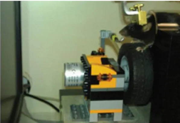
For each training session, the mouse is head-fixed in front of a computer screen with its forepaws resting upon a wheel (Figure 2-1). The mouse can turn the wheel with left or right movements of its forepaws. It can consume droplets of water dispensed via a spout close to its mouth. A nearby speaker can play auditory stimuli.

Figure 2-1 Training setup used for wheel tasks.

Mice were head-fixed with their forepaws resting on a wheel, and their body resting in a tube. Visual stimulation was provided on a screen in front of the animal and water spout near their mouth delivered water reward. See main text for details.

The task is organised into successive trials in which stimuli are presented from one of two discernible categories. The mouse is then required to respond with an appropriate wheel turn. The overall turn direction distinguishes it as a left or right

(27)

27 response, one of which is correct for that trial’s stimulus category. For correct responses, the mouse receives a water reward (typically 2-3 µL). For incorrect responses, a white noise sound is played during a timeout period.

2.2 Version 1: a simple transient stimulus task

I first attempted to train mice with this technique on a simple task with stimuli presented transiently. I trained them five consecutive days each week during which they only received water as a task reward (typically 0.1-0.9 ml per day, depending on proficiency and motivation). During the two day rests they had free access to water. On each trial, mice were presented with a grating disc (Gabor, see 2.1) for 250-500 ms on the left or the right of the screen together with a low or high frequency pure tone (7 or 12 kHz 200 ms pure tone). The stimuli were consistently paired: the left grating with the low tone; the right grating with the high tone. Mice had 4 s to respond by turning the wheel. Left turns were correct for the left/low stimuli; right turns were correct for the right/high stimuli. Turns after stimulus onset were registered as responses when the speed was above ~40 mm/s. The threshold was optimised by trial and error, informed by typical speeds of small and large wheel turns by mice and choosing it to pick out the faster turns mice were able to make. Missed trials were repeated. Incorrect trials were also repeated to discourage a strategy of turning the wheel in one direction (which would otherwise reap a reward on half of the trials). During the first 2-3 training days, rewards were given for responses in either direction.

(28)

28

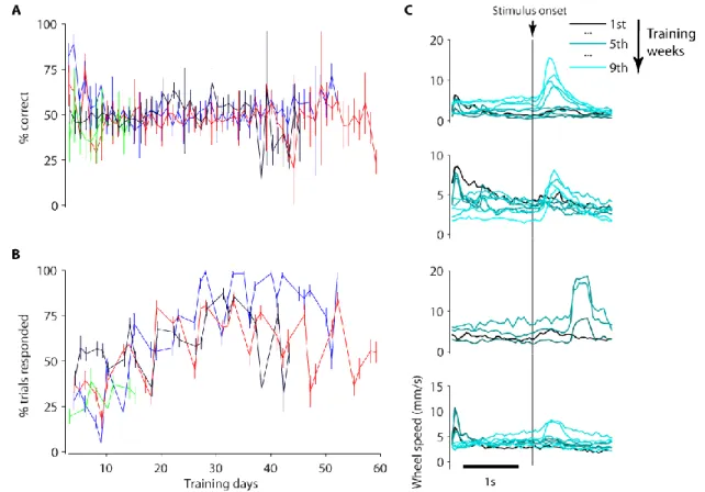
Figure 2-2 Mice failed to learn version 1 of perceptual discrimination task.

A, Percentage correct trials as a function of training day for four mice (different colours). Chance level is 50%. Error bars show 95% binomial proportion confidence interval. The first three training days are not shown as turns in both directions were rewarded. B, Percentage of trials in which mice responded as a function of training day for same mice as in A. The response window is 0-4 s after stimulus onset. Error bars show 95% binomial proportion confidence interval. C, Wheel speed averaged around stimulus onset time over training weeks (graded colours, see legend). Panel rows show the four mice in A.

I implanted four mice then trained them on this task for up to 60 days. Over this period, their responses never surpassed chance-level performance (Figure 2-2A). During latter training weeks, I tested various modifications to make the stimulus more salient (including longer presentation times and making the gratings flicker or drift), but none made a difference to performance. Nonetheless, mice became more

(29)

29 efficient at obtaining rewards as they changed aspects of their behaviour throughout training. Naïve mice quickly learned to turn the wheel, but initially in just one direction. This caused them to become stuck, repeating trials (requiring a counter turn) without rewards. However, over 1-2 training weeks their turn directions became progressively less biased, ultimately enabling them to collect rewards on ~50% of trials. They also learned to initiate their turns after stimulus onset (Figure 2-2C), leading to swifter rewards with fewer turns. This panel also shows that the stimulus-cued response times varied across mice, but did not change with training once acquired. The loss of bias and acquisition of stimulus-cued responses together led to an increase in the fraction of trials with responses over training (Figure 2-2B). These results were encouraging as they showed that mice could competently use a wheel as response device, cued by stimuli. However, they suggested that mice were struggling to relate the direction of their turns to stimulus properties in the task.

2.3 Version 2: using stimulus interactivity to aid learning

In 2.2, mice had failed to associate a stimulus property (in this case visual stimulus position or tone frequency) with their wheel turns. I hypothesised that coupling their actions to changes of the property might help them to form such an association. If they were able to manipulate the property’s value along the relevant dimension with their wheel turns then their goal could be to aim the property toward a target value. For example, for visual stimulus position, the stimulus could be presented on the left or the right of the screen as in the previous task, but now the rewarded goal could be to bring the stimulus to the centre, ahead of them. This in

(30)

30 particular, might also benefit from a similarity to natural appetitive behaviour, akin to orienting toward rewarding objects in the environment.

To investigate this rationale as a solution, I developed the following basic design for a new task:

On each trial, a target stimulus is initially presented on the left or the right of the screen. Wheel turns by the mouse translate the stimulus horizontally: left turns move the stimulus to the left; right turns move the stimulus to the right. The mouse’s goal is to bring the stimulus to the centre of the screen, whereupon the stimulus locks into place and the mouse receives a reward. If instead the mouse translates the stimulus the same distance in the wrong direction, it locks into place there (at the side of the screen) and a white noise sound is played for 2 s to indicate that there is a timeout period. In either case, the stimulus remains locked in its response position for 1-2 s to remind the mouse of its action while it is receiving its feedback, and then disappears.

I applied this basic design in different versions of the task, each with specific stimulus details, timings and conditions. The details of the first version I tested are as follows (also see Figure 2-3).

Methods

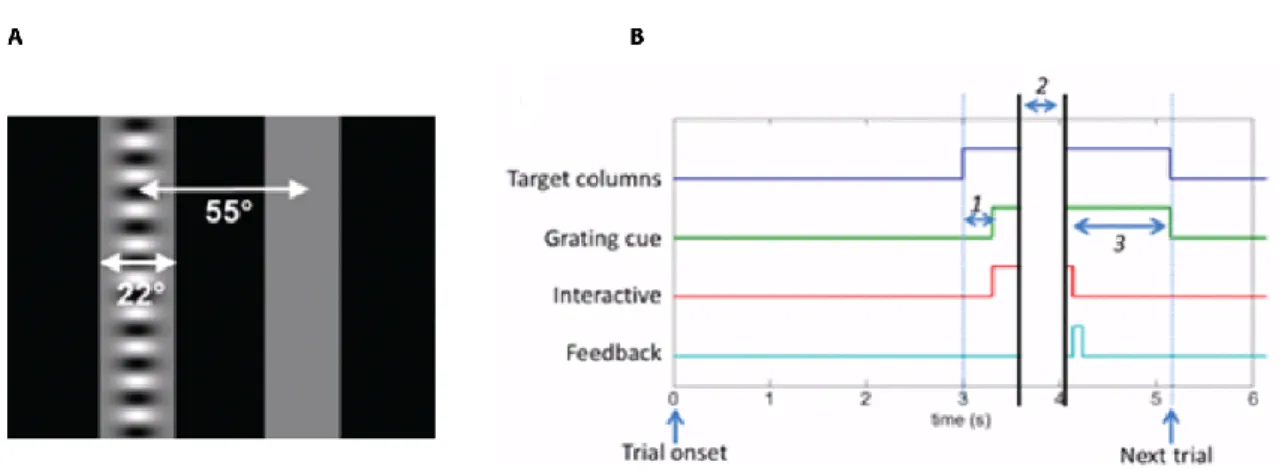
Between trials, the screen was black. After trial onset, two grey columns (22° wide, 55° apart), were presented on the left and right of the screen (Figure 2-3B). Next (300 ms later), a horizontal grating (0.1 cycles/°) was superimposed onto one column and all stimuli became movable (interactive). The rewarded goal was to get

(31)

31 the grating to the centre. There was no response timeout. The inter-trial interval was 3 s.

Figure 2-3 A task using visual feedback to aid learning.

A, Visual stimuli used in the first version of ChoiceWorld as seen on the screen (see main text). The stimuli are translated horizontally by the mouse’s wheel turns, in the direction of its turns. Stimuli dimensions are indicated by the arrows. B, Temporal sequence of events in the task.

Feedback is either the delivery of water reward (for correct trials), or the onset of the 2 s white noise sound (for incorrect trials). Refer to main text for more details.

Results

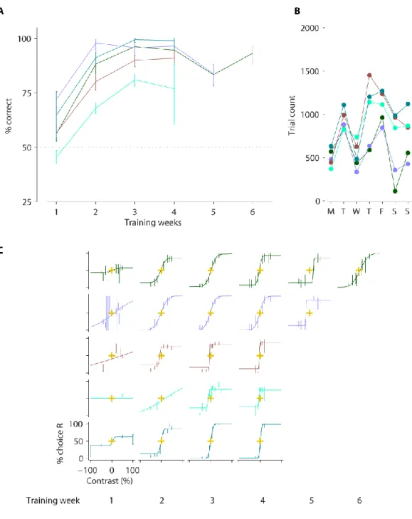
I implanted head-plates in five new mice, and trained them on this task with the same five day training and water restriction schedule as in 2.2 for up to 11 weeks. Mice learned to perform the task with high accuracy (Figure 2-4A). Through the course of each five day water restriction term, mice were increasingly motivated, typically performing few trials on the first water restriction day and the most trials on the last two days (Figure 2-4B, upper panel). Most mice also took longer to complete their responses on Mondays, but there was no effect on other days (Figure 2-4B, lower panel). They were performing above chance by the second or third week so I

(32)

32 gradually introduced lower contrast trials. On the easiest, high contrast trials, proficient mice performed up to 90% of trials correctly, and performed up to 300 trials per day in sessions lasting 30-45 mins.

(33)

33

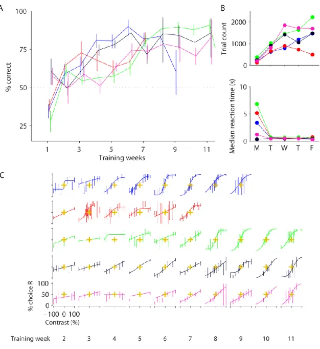
Figure 2-4 Mice learned to correctly report stimuli once visual interaction was introduced (task version 2).

Data from five mice are shown (colour-coded). A,Percentage of correct trials by training week for the easiest trials (the highest contrast trials in each session). Performance was consistently above chance after 3-5 weeks of training. Dashed line indicates chance level. B, Number of trials mice completed, and median reaction time by day of week. Mice were water restricted and trained on weekdays but had free access to water at weekends. C, Psychometric functions for contrast by week (panel columns). The proportion of trials that the mouse chose the right-hand grating (choice R) is plotted as a function of the signed grating contrast, where the sign represents grating position (negative for left-hand side, positive for right-hand side). Task was as described in the main text and Figure 2-3. All error bars show 95% binomial proportion confidence interval.

(34)

34 I analysed their choices as function of stimulus contrast and fitted psychometric functions to the data. The functions are determined by three parameters: lapse rate, contrast bias, and contrast threshold. The parameters each pertain to different aspects of animal choices. The lapse rate reflects the proportion of trials with choices made independent of the stimulus. The contrast bias denotes the contrast at which choices are balanced, i.e. 50% to the left and right. The contrast threshold reflects contrast sensitivity: the lower the threshold, the sharper the modulation of choices by contrast.

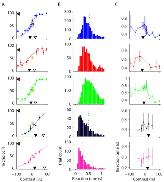
I obtained psychometric functions across training weeks to chart learning (Figure 2-4C). As training progressed, psychometric functions stabilised, eventually producing consistent contrast thresholds, and small biases in later weeks. I pooled data across these weeks for more detailed behavioural analysis (Figure 2-5). In the psychometric analyses (Figure 2-5A), the psychometric functions are plotted along with their parameters. Three mice have similar contrast thresholds (~35%; top three panels, Figure 2-5A) but the other two have relatively high thresholds (> 50%).

Reaction times were largely distributed between 0.1-1 s (Figure 2-5B) but with a long tail ranging up to 40 s due to not enforcing a response time limit. In 3/5 mice, there was a trend for slower reactions on the lowest contrast trials (top three panels in Figure 2-5C). Furthermore, in those mice, the slowest reaction times tended to follow the contrast bias (obtained from the psychometric functions).

(35)

35

Figure 2-5 Behavioural analysis of data from proficient mice in task version 2.

Pooled analyses of last 1-3 training weeks (with stable performance) of mice in Figure 2-1. A, Contrast psychometric functions. Filled black triangles indicate the contrast bias (the contrast at which the mouse chose the left and right equally). Difference in contrast between open and filled black trials indicates the contrast threshold. Red/black triangles indicate the lapse rate (proportion of guessed trials) by their decrement below 100% choice R. Gold crosses show 0% stimulus contrast and 50% choice intersection point for reference. Error bars show 95% binomial proportion confidence intervals. B, Reaction time distribution (time to reach the wheel turn response threshold from grating onset). Vertical dashed line indicates median reaction time. C, Reaction time as a function of grating contrast and position. Data points indicate medians and error bars show 40th_{and 60}th_{percentiles. Contrast biases from}_{A are shown for reference (filled}

(36)

36 These results support the hypothesis that enabling mice to interactively move the stimulus with the wheel helped them learn to direct their turns according to stimulus position.

Task refinements

From a purely behavioural perspective, the new task was successful in that mice were able to learn it and to generate high quality psychometric data. However, for relating stimuli and behaviour to visual neural responses, the task design presented a number of issues.

One issue was the complexity of the visual stimulation: a number of stimulus attributes changed close together in time. There was stimulation both from the target grating and the grey columns. Furthermore, the appearance of grey columns on a black screen caused a large change in overall mean luminance, which is known to invoke retinal adaptation (Barlow and Levick, 1969) and affect psychophysical contrast thresholds (Kilpeläinen et al., 2011). Separating out these factors in neural responses would present additional challenges, particularly with calcium imaging, which has a relatively low temporal resolution (e.g. GCaMP6m transients are reported to peak after ~0.1 s and half-decay in ~0.4 s, Chen et al., 2013). Interpreting neural responses would be more straightforward if the only stimulus change was the appearance of the target itself.

More problematically, the presentation of the target stimulus was poorly controlled. Mice were able to start moving the target as soon as it appeared. Firstly, this complicates comparison between trials, as each stimulus trajectory is controlled

(37)

37 by the mouse. Moreover, any attempt to study the relationship between choice and neural activity is confounded by the introduction of a direct correlation between choice and stimulus movement. One solution to both these issues could be to only analyse trials where the turn (and therefore the stimulus movement) starts late. However, this might introduce other unintended confounds by selecting atypical trials, which might e.g. be those with lower contrasts or where the mouse is satiated. In practice this would also severely limit the number of trials available for analysis, again because proficient mice initiate their responses swiftly (see Figure 2-5B). If however, the target stimulus was made unmovable for a brief period at presentation, neural responses would be controlled in that window.

Finally, there was a fixed delay between the offset of one stimulus and the onset of the next. With a recording technique that uses with low resolutions such as GCaMP calcium imaging, a fixed delay could make it difficult to disambiguate offset and onset responses to visual stimuli. A randomised interval would solve this problem.

2.4 Version 3: controlled stimuli

To address these issues, I developed a new version of the task. To eliminate the mean luminance change and reduce stimulus complexity, the screen background was made grey and the grey columns were abolished. In this version, the target grating was the only stimulus presented. Previously, the grey columns had acted as a cue for the mouse to make a choice. To replace that, I added a tone, presented 500ms before target onset. To better control stimulus presentation, the target was

(38)

38 held in its initial position and did not become interactive until 1 s after onset. To help separate offset and onset responses, a random inter-stimulus interval was introduced, picked on each trial from a uniform distribution between 2-5 s.

Results

I implanted two new mice and trained them on this version. These mice were trained and water restricted seven days a week, receiving a minimum daily amount by topping up any deficit from task rewards (see 2.1). In collaboration with Adam Ranson, we also implanted and trained another three mice and performed two-photon calcium imaging on them. However, due to technical issues with the recordings (including degradation in indicator expression and cell health, see 6.3) the imaging data are not presented in this thesis. Details of the two-photon calcium imaging methods and results from other experiments can be found in Chapter 3.

I started the training with high contrast trials, and short inter-stimulus (1 s) and interactive intervals (0-0.5 s). As training progressed these were increased to their final durations (more details can be found in 2.1).

(39)

39

Figure 2-6 Rapid acquisition of task version 3.

Data from five mice are shown (colour-coded). A,Percentage of correct trials by training week for the easiest trials (the highest contrast trials in each session). Performance was consistently above chance by the second week of training. Dashed line indicates chance level. B, Number of trials mice completed by day of week. Mice were water restricted and trained seven days a week without free water breaks. C, Psychometric functions for contrast by week (panel columns). The proportion of trials that the mouse chose the right-hand grating (choice R) is plotted as a function of the signed grating contrast, where the sign represents grating position (negative for left-hand side, positive for right-hand side). Task was as described in the main text. All error bars show 95% binomial proportion confidence interval.

(40)

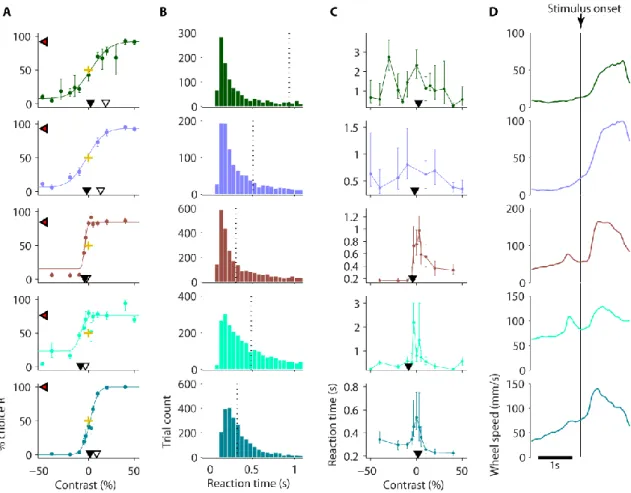
40 Mice learned to perform this task proficiently after 2 weeks of training (Figure 2-6A). For some mice, performance on the easiest trials dropped in later weeks of training after being given a particularly large proportion of difficult (low contrast) trials. With the continuous training schedule there was no trend by training day for motivation (Figure 2-6B). High-quality contrast psychometric functions were typically produced from the second week onwards, and were stable across weeks (Figure 2-6C), producing psychometric curves with little bias and similar contrast thresholds. As with the previous version, I performed a detailed behavioural analysis of data pooled data across these the weeks (Figure 2-7). The psychometric analyses revealed generally lower contrast thresholds and biases than in the previous task (Figure 2-7A vs Figure 2-5A, and also see the summaries in Figure 2-9). As in the previous version, reaction times were generally slower for more difficult trials (i.e. lower contrast).

This cohort learned faster and performance was more reliable sooner than those in the previous task version (Figure 2-6A vs Figure 2-4A). Although I did not investigate this further, this could be for a number of reasons including more careful training, the improved training and water schedule (supported by stabilised motivation, Figure 2-6B) and also the simpler stimulus (since mice were only presented with one stimulus in this version, they did not need to learn which was the important one).

(41)

41

Figure 2-7 Behavioural analysis from mice proficient in version 3 of the task.

Pooled analyses of all sessions from the third week of training onwards of mice in Figure 2-6. A, Contrast psychometric functions. Filled black triangles indicate the contrast bias (the contrast at which the mouse chose the left and right equally). Difference in contrast between open and filled black trials indicates the contrast threshold. Red/black triangles indicate the lapse rate (proportion of guessed trials) by their decrement below 100% choice R. Gold crosses show 0% stimulus contrast and 50% choice intersection point for reference. Error bars show 95% binomial proportion confidence intervals. B, Reaction time distribution (time to reach the wheel turn response threshold from interactive, 1 s after grating onset). Vertical dashed line indicates median reaction time. C, Reaction time as a function of grating contrast and position. Data points indicate medians and error bars show 40th_{and 60}th_{percentiles. Contrast biases from}_{A are shown for}

reference (filled black triangles). D, Wheel speed averaged around stimulus onset time.

The modifications now meant a single stimulus change on each trial, a period with controlled stimulus position, and a randomised separation between stimulus

(42)

42 offsets and onsets. After obtaining these results, I became more confident that the general principles that informed the design of the task were actually responsible for the good performance in the task and that specific details could be changed without adversely affecting performance.

2.5 Version 4: controlling wheel movements

I had two more potential concerns with measuring neural activity during the task that I wanted to address. One concern was the issue of uncontrolled movements of the mouse before stimulus onset. It is known that neural responses in V1 are affected by running (Ayaz et al., 2013; Keller et al., 2012; Saleem et al., 2013). If the effects of wheel movements are similar it may complicate interpretation of responses: in 2.4, mice tended to be making significant wheel movements in the period leading up to stimulus presentation (Figure 2-7D). The other concern was that the vertical extent of the stimulus (65°) would evoke responses over large strip of V1. I hypothesised that, given a fixed pool of neurons that can be recorded, the more neurons that carry information about the stimulus, the less likely it is that the recorded ones will be carrying a significant proportion of the information guiding further processing and decision-making. Thus, it may be preferable restrict the size of the target stimulus.

To address these concerns, I made the following modifications. To control for wheel movement at stimulus onset, I introduced a 2-3 s quiescence period: a random duration was picked for each trial uniformly from 2-3 s, and each stimulus was not presented until mice had not moved the wheel for the full duration. To shrink the

(43)

43 population of neurons that respond to the stimulus, I used a circular Gabor grating (standard deviation 7.5°; ~18° full width half maximum) instead of the grating column. This size ensured that at least grating two cycles of the grating were visible when presented at 0.1 cyc/° (this spatial frequency is approximately the peak of mouse contrast sensitivity, Histed et al., 2012). In this version, the onset tone was presented 100 ms before the visual stimulus.

Results

I trained three new mice on this version and learning proceeded at a similar rate to the previous task (Figure 2-8A) with proficient mice performing the easiest trials at ~90% accuracy. Their psychometric functions had stabilised by the third week of training and produced high quality psychometric curves (Figure 2-8B).

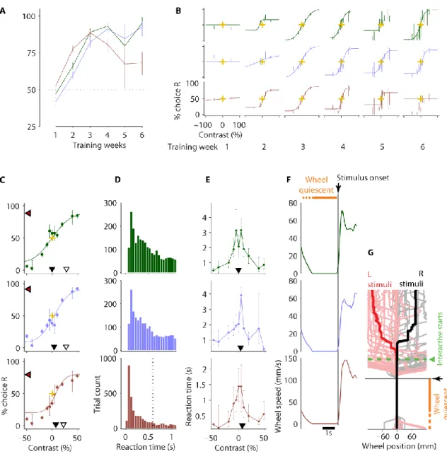
A detailed analysis of data obtained from the third week onwards (Figure 2-8) showed similar contrast thresholds and biases to the previous version (Figure 2-8C vs Figure 2-7A, and summaries in Figure 2-9). Contrast thresholds were slightly increased, presumably due to the stimulus being smaller. Median reaction times were slower, but the fastest reaction times were quicker (Figure 2-8E vs Figure 2-7B), possibly because of the state of readiness facilitated by the enforced quiescent period before stimuli. Possibly related to this, reaction times showed a much clearer trend for slower times with decreasing contrast (Figure 2-8E).

(44)

44

Figure 2-8 Task acquisition and stable psychometrics in version 4.

Data from three mice are shown (colour-coded). A,Percentage of correct trials by training week for the easiest trials (the highest contrast trials in each session). Dashed line indicates chance level. B, Psychometric functions for contrast by training week (panel columns). C-F, Pooled analyses of sessions from the third week onwards. C, Contrast psychometric functions. Filled black triangles indicate the contrast bias (the contrast at which the mouse chose the left and right equally). Difference in contrast between open and filled black trials indicates the contrast threshold. Red/black triangles indicate the lapse rate (proportion of guessed trials) by their decrement below 100% choice R. Gold crosses show 0% stimulus contrast and 50% choice intersection point for reference. Error bars in A-C show 95% binomial proportion confidence intervals. D, Reaction time distribution (time to reach the wheel turn response threshold from interactive, 1 s after grating onset). Vertical dashed line indicates median reaction time (out of bounds in top two panels). E,

(45)

45

Reaction time as a function of grating contrast and position. Data points indicate medians and error bars show 40th_{and 60}th_{percentiles. Contrast biases from C are shown for reference (filled}

black triangles). F, Wheel speed averaged around stimulus onset time. G, Wheel trajectories relative to stimulus onset time (black arrow and horizontal line) grouped by stimulus position (red for left stimuli; black for right stimuli). Two thick traces show median position, thin traces show individual trials. Green line and arrow indicates time stimulus became movable (interactive). 2-3 s pre-stimulus quiescence period (requisite wheel stillness before stimulus presentation) indicated by orange bars in F-G.

This data showed that the stimulus change (to a circular Gabor grating) and the imposition of the pre-stimulus quiescence period did not impact learning acquisition or overall performance. Moreover, the quiescence period was now prominently displayed by the complete lack of wheel movement leading up to stimulus onset in the wheel trajectories (Figure 2-8F vs Figure 2-7D). This is highlighted in a plot of individual and median wheel trajectories relative to stimulus onset time grouped according to stimulus position (Figure 2-8G). This plot also shows that mice in this task did not tend to wait for the stimulus to become interactive (green line 1s after stimulus onset) before initiating their responses.

In collaboration with Adam Ranson, these mice were also injected with GCaMP6m virus, and imaged while they performed the task. The imaging results are discussed further in Chapter 3.

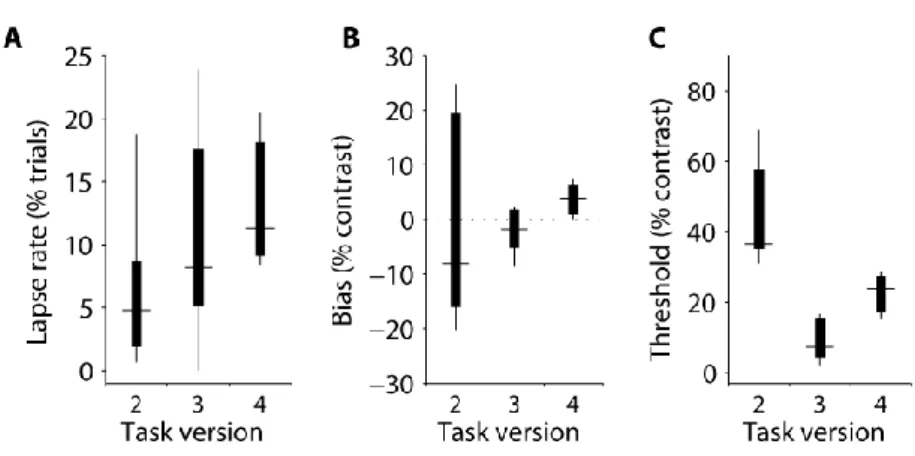
Finally, to enable comparison of psychophysical performance obtained across the different tasks (and with other studies), I compiled summary statistics of the psychometric function parameters across all the animals trained in task version 2-4 (Figure 2-9). Contrast thresholds were considerably higher in version 2, presumably

(46)

46 because of the presence of other stimulus changes which the mice had to ignore, including a large mean luminance change at stimulus onset, which will invoke adaptation. Biases were smaller and more consistent in task versions 3 and 4. Thresholds were generally higher for task version 4, possibly because the stimulus is smaller than in task version 4 (and the narrow grating column used in version 3 is unlikely to invoke considerable surround suppression) although more data would be needed to support this conclusion.

Figure 2-9 Psychometric parameters across task versions.

Summary of parameters from model fits to contrast psychometric data of all mice by task version. A, Lapse rates (percentage of trials in which the stimulus is ignored and the mouse guesses). B, Contrast bias (the contrast at which the mouse made an equal proportion of left and right choices). C, Contrast threshold (the contrast increment required to go from equal choices to ~84% of the upper bound in right-hand stimulus choices; upper bound is 100% minus the lapse rate). Data are summarised in box plots: horizontal bars are medians, box edges are 25th_{and 75}th_{percentiles and}

(47)

47

2.6 Discussion

I have described the development of an effective two-alternative forced choice task for head-fixed mice. First, I showed that mice were not able to learn the task under a simpler regime where stimulus properties were unconnected to wheel movements except via subsequent reward. Second, I showed that after giving mice control of stimulus position with the wheel they were able to make visually guided choices and produce high quality psychometric data. Third, I developed the task through a number of iterations that were motivated by improving the interpretation of planned neural recordings during the task. In spite of these changes, behavioural performance remained robust across all iterations.

So why did mice not learn the simple task, but did learn when they were given control over the stimulus? I would speculate that mice lacked the cognitive abilities to form an abstract link between the positions of fixed gratings and the directions of their wheel turns, especially given that the link itself is only reinforced once per trial via operant conditioning. In contrast, in the interactive task, mice receive continuous feedback about their actions with the wheel, which may help form the required link. Furthermore, they can use the wheel to move the stimulus through a continuous space, which may appeal to natural egocentric orienting and grasping behaviours, and their underlying brain mechanisms (Glimcher, 2003; Gnadt and Andersen, 1988; Scherberger and Andersen, 2007).

This is particularly true given that mice had to turn the wheel in the direction they wanted the stimulus to move – forces of the same direction would produce the

(48)

48 same effect in the real world: e.g. to move toward an entity off to the left you apply force to toward the right on the ground to move yourself left, or, to bring an entity on your left toward your fore, you should apply a force its right. Furthermore, the mice were rewarded for bringing an initially distal stimulus to their fore, which is an appetitive-like behaviour.

A variety of different sensory guided tasks have been developed for mice, each with their own subset of features and ideal applications. This includes a freely moving two-alternative forced choice paradigm (Busse et al., 2011), and head-fixed go/no go style designs, either in virtual reality (Poort et al., 2015) or with simple, controlled stimulus presentation (Glickfeld et al., 2013; Histed et al., 2012). This task offers a head-fixed two-alternative forced choice (2AFC) paradigm with simple stimuli (and mostly controlled, particularly as the interactivity restricted in time) and relatively rapid learning, making it ideally suited to psychophysical investigation. Sanders and Kepecs, 2012 have published a 2AFC task for head-fixed mice suited to auditory psychophysical measurements, which also uses a wheel-like device controlled the mouse’s forepaws for getting reports.

On its own, this is an effective task for performing head-fixed psychophysical experiments in mice. However, by providing a rigorous a psychophysical measure to relate to neural activity, combining it with neural recordings in sensory cortex makes it possible to investigate sensory contributions to perception. In the next chapter we shall look at V1 activity while mice perform the final variant of the task (version 4).

(49)

49

3 V1 calcium activity during behaviour

3.1 Introduction

My goal was to be able to obtain rigorous psychophysical measurements from mice for comparison with simultaneously measured sensory activity. In the previous chapter, I demonstrated an appropriate task for this purpose, but what is the most suitable recording method? There are two factors stand out as particularly relevant to recordings during perceptual decision-making. One is the value of obtaining significant amounts of data from large populations of the same cells. Analysing patterns of correlations among different sources of variability is a common feature of many of the analysis techniques used in the study of perceptual decision-making. This usually requires a lot of trials or data in general. Another factor is the value of the trained animal. While required training periods are relatively short in the task (especially compared to primates), training mice still requires some time and their performance can be variable across sessions, especially if distressed. This means acute methods are often risky and can be low yield.

GCaMP calcium imaging uniquely addresses these requirements by enabling imaging of the same cells over a period of weeks or more (Chen et al., 2013; Madisen et al., 2015). I chose to use calcium imaging for these reasons. However, it is also important to be aware of, perhaps, its chief limitation: temporal resolution. This significantly improved with the availability of the GCaMP6 family (Chen et al., 2013). However, for certain questions electrical recordings are still the best method,

(50)

50 particularly those concerning temporal aspects of sensory coding or the timing of information flows during perceptual decisions.

I collaborated with Adam Ranson to perform two-photon calcium imaging of V1 in mice engaged in the task.

3.2 Methods

I performed behavioural methods including, water restriction schedule, training procedure, stimulus delivery and psychometric analysis as described in 2.1. Specifically task version 4 (see 2.5) was used in all experiments described in this chapter.

Intrinsic signal mapping of retinotopy

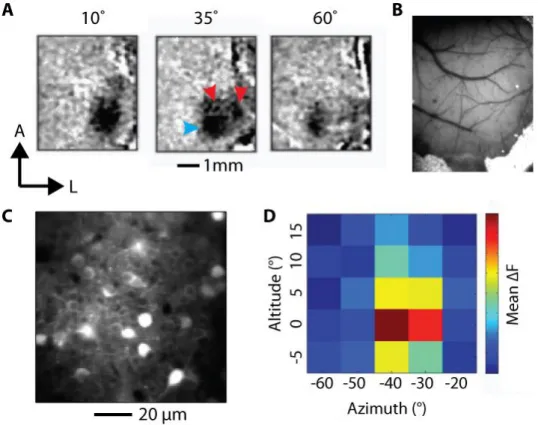
To ensure expression of GCaMP in a V1 region with receptive fields covering the onset position of the task stimulus, we obtained stereotaxic coordinates for virus injections using intrinsic signal mapping (Grinvald et al., 1986) in two mice. We anaesthetised the mice with isoflurane and presented them with drifting gratings while the right cortex was illuminated with green light (530±20 nm; Thorlabs LED) and imaged (PCO camera) at 10 Hz. The gratings were randomly centred at one of three different azimuths along the horizontal meridian in the left visual hemi-field. We computed mean haemodynamic response maps to stimuli in each position from the imaging frames. We measured the stereotaxic coordinates at the centre of the V1 response patch (blue arrowhead in Figure 3-1A) to the middle grating, which corresponded to the onset position of the left target stimulus used during training.

(51)

51 We obtained mean stereotaxic coordinates of 2.8 mm lateral and 3.3 mm caudal to bregma (right hemisphere).

Expressing GCaMP in V1 neurons

We anaesthetised three 10-12 week old C57BL/6J female mice with isoflurane and implanted them with a metal head plate attached to the skull. We performed a 1mm2_{craniotomy in the middle of a circular aperture in the head plate. The}

craniotomy was centred in the right cortex at the stereotaxic coordinates obtained from the intrinsic signal mapping experiment (see above). We then injected them with GCaMP6m virus (AAV2/1-syn-GCaMP6m-WPRE, adeno-associated virus with human synapsin promoter driving expression of GCaMP6m, undiluted 2x1013

genome copy/ml from Penn Vector Core; Chen et al., 2013) into the centre of the craniotomy at a depth of 250 µm beneath the dura. We then covered the craniotomy with a two-layer glass coverslip construction, and sealed it with dental cement. The mice were allowed to recover for 1 week before water restriction and head-fixed training began. Water restriction was on a continuous schedule (see 2.1).

I trained the mice in task version 4 (described in 2.5), a Gabor discrimination task (trial structure is illustrated in Figure 3-2B).

Measuring V1 calcium activity during task performance

I began calcium imaging 3 weeks after virus injection. Imaging was performed using a Sutter two-photon movable objective microscope controlled by ScanImage (Pologruto et al., 2003). A Coherent Chameleon laser running at 1000 nm provided excitation, with power level controlled by a Conoptics pockels cell. Images were

(52)

52 acquired continuously at 12Hz with a resolution of 128×128 pixels. An Olympus 20X object was used for focusing. Imaging data was synchronised with behavioural and stimulus events by simultaneously acquiring signals with imaging frame events and screen refresh events (using a photodiode directly measuring the screen).

In each mouse, I chose a field of view with good GCaMP expression for longitudinal behavioural imaging. I mapped the preferred stimulus position of the field of view by imaging the field of view while repeatedly presenting a grating stimulus on a grey screen (same as in the task) for 1 s with 1-2 s inter-stimulus intervals. Stimuli were presented at positions drawn randomly from a 5×5 grid in the left hemi-field. The mean stimulus response across the field of view was calculated at each stimulus position. The position evoking the largest response was taken as the field of view’s position preference.

I installed the behavioural apparatus under the microscope (illustrated in Figure 3-2A) and imaged the mice while they performed the task. Before behavioural imaging commenced, I shifted the task stimulus onset position to the preferred position of the chosen field of view (the shift was typically < 10°).

Data analysis

I first registered the raw calcium movies using an algorithm that aligns each frame to the peak cross-correlation with a reference frame using the discrete Fourier transform (Guizar-Sicairos et al., 2008). I found cell regions of interest (ROIs) either by hand or by using a semi-automated algorithm that finds nearby pixels that are significantly correlated with each other. ΔF/F calcium signals of ROI traces were

(53)

53 computed as in Jia et al., 2011. Briefly, from calcium traces F, I obtained a measure of baseline F0 by smoothing F in time (0.75s causal moving average) and finding the minimum over a (causal) sliding window (20s). ΔF/F is computed by computed by applying a causal exponentially weighted filter (τ = 0.2 s) to the fractional change (F-F0)/F. In trial-based analyses, I did not use data from repeat trials (trials repeated due to an incorrect choice by the mouse).

For neural decoding I trained support vector machines (SVMs; Cortes and Vapnik, 1995) on vectors of neural activity to linearly classify the stimulus position or choice of trials. I trained and tested classifiers using the svmtrain and

svmclassify MATLAB functions, respectively, in the Statistics Toolbox.

I fitted intervals to bouts of wheel turns in the wheel speed trace using a Schmitt trigger-based dynamic threshold procedure. I adjusted the two thresholds by hand until they appeared to produce good fits the bouts.

I computed movement onset- and offset-triggered average calcium activity from segments of cell ΔF/F traces around the onset or offset events. For each cell I averaged across these ΔF/F segments but I excluded any periods with a stimulus present and until 3 sec after stimulus offset from these averages.

3.3 Results

GCaMP expression in task-stimulus responsive V1 neurons

We performed virus injections in three mice to express GCaMP6 and implanted a chronic imaging window over the area (Figure 2-1A). I then trained the

(54)

54 mice in the Gabor position discrimination task (Figure 3-2B; task version 4 described in 2.5). Once their GCaMP expression was bright and they had achieved stable psychometric performance (after two weeks of training, see Figure 2-8) they were used for two-photon imaging. A field of view was chosen (100x100 µm; Figure 3-1C) and its overall receptive field preference was measured (Figure 3-1D). The preference was used to fine-tune the onset position of the target stimulus to maximise responses in the field of view. I was then able to return to the same field of view over multiple imaging sessions in mice while they performed the task (setup shown in Figure 3-2A).

(55)

55

Figure 3-1 Targeted expression of GCaMP in V1 neurons

A, Intrinsic signal maps used to obtain stereotaxic coordinates for virus injection. Mean responses to stimuli at different positions. Stereotaxic coordinates were obtained from the V1 response patch (blue arrow) was distinguishable from responses in higher visual areas (red arrows). B, Imaging window over V1. C, Example field of view from two-photon calcium imaging chosen for longitudinal imaging. D, Results from retinotopic mapping of the field of view in C. The same Gabor grating used in the task was repeatedly presented in multiple locations. The peak response location was used to position the grating stimulus in the task.

Responses modulated by position and contrast

I typically identified 20-30 cell regions of interest (ROIs) in a given field of view. Among those I found cells with clear calcium transients evoked in response to the contralateral target stimulus (Figure 3-2C).

(56)

56

Figure 3-2 Imaging V1 calcium activity during behavioural task performance

A, Schematic of imaging and behavioural setup. B, Trial structure of the task. The task used was version 4 described in 2.5. C-D, Calcium activity from three example cell regions of interest (A) and wheel turn velocity (B) over time during a typical behavioural recording session. Shaded regions indicate periods with stimuli present and their type (red shading indicate contralateral stimuli, grey shading indicate ipsilateral stimuli; shading intensity and text indicates contrast level). Turn onsets (green triangles) and offsets (red triangles) from a fitting procedure (see main text) are shown on the wheel velocity plot. Magenta asterisks show examples of pre-stimulus activity build-ups; magenta crosses show examples of build-ups in longer intervals between stimuli.

To assess the modulation of V1 cells by task stimuli, I computed trial averages of cell traces (cell ROIs in Figure 3-3A) around grating onset time. These showed a rapid rise in fluorescence following the onset of contralateral stimuli (Figure 3-3B). Responses were at or close to the peak by the time the stimulus became movable (interactive) after 1 s. In contrast, fluorescence typically decayed after ipsilateral stimuli or on blank trials. I found that response amplitude increased with the contrast of contralateral stimuli but was unmodulated by ipsilateral stimulus contrast (Figure

(57)

57 3-3C). The difference in ΔF/F amplitude for the strongest stimuli and blanks ranged between 7-50% (mean 18%±16%).

(58)

58

Figure 3-3 V1 calcium responses modulated by stimulus position and contrast

Calcium activity in response to contralateral (red traces) and ipsilateral (black traces) stimuli presented during behavioural experiments in two mice (row-wise). A, Imaging field of view (showing mean calcium fluorescence across a session), each with three cells delineated (labelled blue circles). B, Mean calcium activity averaged around the onset of the grating stimulus, grouped by stimulus condition (colour-coded lines, see legend) for the three cells (panel columns, blue cell label inset). Orange bar shows part of the period of no wheel movement required before stimuli are presented. Dashed green interactive line indicates the moment the stimulus becomes movable. C, Response amplitudes of each cell to different stimulus contrasts and positions. Amplitude is mean response at 1 s after grating onset. The x-axis is reversed to emphasise that response amplitudes increase with contralateral stimulus contrast.

(59)

59 Decoding task and behavioural variables

Given that both mouse choices and sensory responses were dependent on stimulus position, I was able to ask how they related to one another. In order to compare stimulus coding with psychometric assessments, I measured the reliability of stimulus position decoding from population activity as a function of contrast. To do this, I trained support vector machines (SVMs) to classify stimulus position using pixel vectors of the stimulus response movies (Figure 3-4A). The SVMs were trained on half the trials of a single session, then tested on other unseen trials from the same session or subsequent sessions. I then counted classifications as a function of contrast and position and fitted this data in the same way as with psychometric data (0) to obtain neurometric functions (Figure 3-4B). Compared with the corresponding psychometric functions obtained from mouse choices on the same trials (also in Figure 3-4B), neurometric functions were steeper, indicating higher contrast sensitivity. This suggests mouse choices were not based on all the information available in a just a single imaging field of view. Due to the classifier being trained on neural responses from a single hemisphere, the neurometric functions were more biased than mouse choices (see 6.4 for explanation), and consistently to the left (i.e. the contralateral side; see response bias in Figure 3-3C).

(60)

60

Figure 3-4 Decoding task variables from V1 stimulus responses

A, Schematic of classifier procedure. A support vector machine (SVM) is trained to classify the stimulus position of trials from vectors of calcium imaging movie pixels during the fixed stimulus period (0-1 s following onset). See main text for details. B-C, Population neurometric functions for contrast (solid lines) for two mice (row-wise). Trial stimulus position classifications made by SVMs shown as a function of contrast. A classifier was trained on half the trials within a session and tested on the other half (B). The same classifier was then tested on sessions from two other days (C). Error bars are 95% binomial confidence intervals. For comparison, the psychometric functions obtained from the mouse choices on the same trials are shown (dashed line). D, Classifier performance on decoding mouse choices (cross-validated). SVMs were trained on response movies as in A but in this case to classify mouse choices on a subsets of trials with the same stimulus condition (stimulus-intendent). Error bars show standard deviation obtained by classifying random subsets of trials.