A Study of Time and Energy Efficient Algorithms for Parallel and Heterogeneous Computing

(1)

A Study of Time and Energy Ecient

Algorithms for Parallel and Heterogeneous

Computing

Thesis submitted in accordance with requirements of the University of Liverpool for the degree of Doctor in Philosophy

by

Jude-Thaddeus Ojiaku

September 2016

(2)

Abstract

This PhD project is motivated by the need to develop and achieve better and energy ecient computing through the use of parallelism and heterogeneous systems. Our con-tribution consists of both theoretical aspects, as well as in-depth and comprehensive empirical studies that aim to provide more insight into parallel and heterogeneous com-puting.

Our rst problem is a theoretical problem that focuses on the scheduling of a special category of jobs known as deteriorating jobs. These kind of jobs will require more eort to complete them if postponed to a later time. They are intended to model several industrial processes including steel production, re-ghting and nancial management. We study the problem in the context of parallel machine scheduling in an online setting where jobs

have arbitrary release times. Our main results show that List Scheduling is(1 +bmax)

-competitive and that no deterministic algorithm is better than (1 +bmax)1−m1 , where

bmax is the largest deteriorating rate. We also extend our results to online deterministic

algorithms and show that no deterministic online algorithm is better than (1 +bmax)

-competitive.

Our next study concerns the scheduling ofnjobs with precedence constraints onm

par-allel machines. We are interested in the precedence constraint known as chain precedence constraint where each job can have at most one predecessor and at most one successor. The jobs are modelled as directed acyclic graphs where nodes represent the jobs and edges represent the precedence constraints between jobs. The jobs have a strict deadline that must be met. The parallel machines are considered to be unrelated and a commu-nication network connects each pair of machines. Execution of the jobs on the machines as well as communication across the network incurs costs in the form of time and energy. These costs are given by cost matrices that covers processing and communication. The goal is to construct a feasible schedule that minimizes the total energy required to ex-ecute the chain of jobs on the machines, such that all deadlines are met. We present a dynamic programming solution to the problem that leads to a pseudo polynomial time

(3)

ii

algorithm with running time O(nm2dmax), wheredmax is the largest deadline. We show

that the algorithm computes an optimal schedule where one exists.

We then proceed to a similar problem that involves the scheduling of jobs to minimize ow time plus energy. This problem is based on a dynamic speed scaling heuristic in literature that is able to adjust the speed of a processor based on the number of active jobs, called AJC. We present a comprehensive empirical study that consists of several job selection, speed selection and processor allocation heuristics. We also consider both single processor and multi processor settings. Our main goal is to investigate the viability of designing a xed-speed counterpart for AJC, that is not as computationally intensive as AJC, while being very simple. We also evaluate the performance of this xed speed heuristic and compare it with that of AJC.

Our fourth and nal study involves the use of graphics processing unit (GPU) as an accel-erator for compute intensive tasks. The GPU has become a very popular multi processor for heterogeneous computing both from an economical point of view and performance standpoint. Firstly, we contribute to the development of a Bioinformatics tool, called GapsMis, by implementing a heterogeneous version that uses graphics processors for ac-celeration. GapsMis is a tool designed for the alignment of sequences, like protein and DNA sequences, and allows for the insertion of gaps in the alignment. Then we present a case study that aims to highlight the various aspects, including benets and challenges, involved in developing heterogeneous applications that is vendor-agnostic. In order to do this we select four algorithms as case studies including GapsMis and the algorithm presented in our second problem. The other two algorithms are based on the Velocity-Verlet integration and the Fruchterman-Reingold force-based method for graph layout. We make use of the Open Computing Language (OpenCL) and C++ for implementa-tion of the algorithms on a range of graphics processors from Advanced Micro Devices (AMD) and NVIDIA Corporation. We evaluate several factors that can aect perfor-mance of these applications on each hardware. We also compare the perforperfor-mance of our algorithms in a multi-GPU setting and against single and multi-core CPU implementa-tions. Furthermore, several metrics are dened to capture several aspects of performance including execution time of application kernel(s), execution time of application including communication times, throughput, power and energy consumption.

(4)

Acknowledgements

Firstly I would like to show my deepest gratitude to my supervisors Dr. Prudence Wong and Prof. Leszek G¡sieniec for their support and advice throughout the duration of my PhD studies. I have learned a lot during this period and they have always guided me in the right direction.

I am very grateful to my family for their unending love, encouragement and support, and for giving me the means to ensure that I complete my PhD studies.

I would also like to thank all my friends and colleagues for their help and support including Dr. O. Nwamadi, whose help, discussions and advice beneted me a great deal.

(5)

List of Figures

1.1 An illustration of linear deterioration. . . 7

1.2 Examples of job precedence constraints. . . 10

2.1 An illustration of jobs based on the deteriorating rates. . . 19

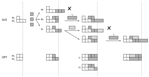
2.2 An illustration of schedules constructed by LS and OPT for the job set shown in Figure 2.1. . . 19

2.3 An illustration of n jobs assigned to one machine. . . 20

2.4 Stage 1 of adversary: The deteriorating rate,b1, of jobJ1 satises1 +b1 = (1+b)3wherebis the deteriorating rate of each of the smaller jobs depicted in the illustration. Jobs are released at time t0 and scaled according to deteriorating rates only. . . 21

2.5 Stages 2 and 3 of adversary: (A) In stage 2, jobs are released at time t1=t0(1 +b1)and as a result, LS cannot schedule them earlier onM1and M2. This means machinesM1 andM2 are idle until timet1. (B) In stage 3 new jobs start arriving at time t2 =t1(1 +b2) and the trend continues as with the previous stages. . . 22

2.6 Illustration of the 3 representative cases, labelled (a), (b) and (c), in stage 2 of the general lower bound. . . 25

2.7 Example showing Stage 3 of the general lower bound. . . 25

2.8 Illustration of the general lower bound for Stage 31 where k = 31 and h = 15. (i) At t30 ALG is still processing J30 from Stage 30 on M1. (ii) OPT has completed all jobs released before t30 including J30. (iii) OPT schedule for Stage 31. Note that OPT can maintain the same makespan on both machines. . . 26

4.1 Class diagram of the simulator software program. . . 44

4.2 Details of the Job and JobGenerator classes. . . 45

4.3 Details of the scheduler part of the simulator. . . 46

4.4 Measurement shows the ratio of total ow time plus energy for SJF vs AJC on a single processor. Results are grouped according to average job size. . . 47

4.5 Measurement shows the ratio of total ow time plus energy for SJF vs AJC on a single processor. Results are grouped according to average inter-arrival time. . . 48

4.6 Measurement shows the ratio of total ow time plus energy for SJF vs AJC on 4 processors. Results are grouped according to average job size. . 50

4.7 Measurement shows the ratio of total ow time plus energy for SJF vs AJC on 4 processors. Results are grouped according to average inter-arrival time. 51

(9)

List of Figures viii

4.8 Eectiveness of speed scaling: Measurement shows the ratio of total ow time plus energy for a xed speed heuristic using a speed of 1 against AJC on a single processor. Results are grouped according to average job size. Note: ratio is always at least 1. . . 52

4.9 Eectiveness of speed scaling: Measurement shows the ratio of total ow time plus energy for a xed speed heuristic using a speed of 1 against AJC on a single processor. Results are grouped according to average inter-arrival time. Note: ratio is always at least 1.. . . 53

4.10 Speed scaling vs.semi-clairvoyant xed speed function: Measurement shows the ratio of total ow time plus energy between AJC and a xed speed function that has some information about the job set. Results are grouped according to average job size. . . 59

4.11 Speed scaling vs.semi-clairvoyant xed speed function: Measurement shows the ratio of total ow time plus energy between AJC and a xed speed function that has some information about the job set. Results are grouped according to average inter-arrival time. . . 60

4.12 Eectiveness of AJC speed spectrum: Comparison of AJC to a xed speed function that uses, as xed speed values, the average and maximum speeds obtained from a prior AJC run. Results show the performance ratio of the total ow time plus energy of xed speed functions vs.AJC. . . 61

4.13 Eectiveness of AJC speed spectrum: Comparison of AJC to a xed speed function that uses, as xed speed values, the average and maximum speeds obtained from a prior AJC run. Results show the performance ratio of the total ow time plus energy of xed speed functions vs.AJC. . . 62

4.14 Results for RoundRobin in terms of average job size comparing the performance ratio of total ow time plus energy for a single processor vs.multiple processors. . . 63

4.15 Results for RoundRobin in terms of average inter-arrival time comparing the performance ratio of total ow time plus energy for a single processor vs.multiple processors. . . 64

4.16 Results for *MinActiveCount in terms of average job size comparing the performance ratio of total ow time plus energy for a single processor vs.multiple processors. . . 65

4.17 Results for *MinActiveCount in terms of average inter-arrival time comparing the performance ratio of total ow time plus energy for a single processor vs.multiple processors. . . 66

4.18 Results for *MinCost in terms of average job size comparing the perfor-mance ratio of total ow time plus energy for a single processor vs.multiple processors.. . . 67

4.19 Results for *MinCost in terms of average inter-arrival time comparing the performance ratio of total ow time plus energy for a single processor vs.multiple processors. . . 68

4.20 Results for *MinSize in terms of average job size comparing the perfor-mance ratio of total ow time plus energy for a single processor vs.multiple processors.. . . 69

4.21 Results for *MinSize in terms of average inter-arrival time comparing the performance ratio of total ow time plus energy for a single processor vs.multiple processors. . . 70

(10)

5.1 A fundamental dierence between a CPU and a GPU is that the GPU

dedicates majority of its transistors to execution units. . . 74

5.2 Thread divergence occurs as a result of threads within a wavefront/warp taking dierent code paths. . . 76

5.3 Thread divergence can be avoided if branch granularity of the GPU hard-ware is maintained. . . 77

5.4 The GPU is able to hide latency by swapping out wavefronts/warps that stall during memory operations. . . 78

5.5 Non-coalesced memory access patterns can result in poor performance on the GPU hardware.. . . 79

5.6 Coalesced memory access patterns can improve performance on the GPU hardware. . . 79

5.7 Generalized block diagram of AMD's GCN architecture. . . 80

5.8 Generalized block diagram of NVIDIA's Kepler architecture. . . 81

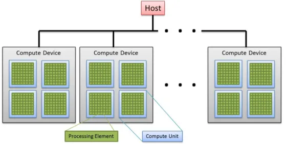
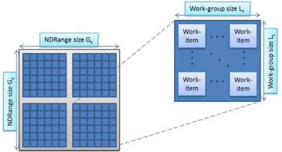
5.9 Block diagram illustrating the major components of the OpenCL platform. 83 5.10 Decomposition of an OpenCL index space into work-groups and work-items. 84 5.11 Illustration of the OpenCL memory model. . . 85

6.1 Illustration of how the NDRange is dened so that work-groups are mapped to machines in the input and a work-item maps to a time index.. . . 94

6.2 An example showing the advantage of using vector data type. (a) Without vectors, work-items need 4 memory accesses in order to retrieve values from tables. (b) Using vectors, two read operations are merged into a single read. . . 95

6.3 Alignment with no gap. . . 97

6.4 Alignment with 1 gap. . . 97

6.5 Alignment with 2 gaps.. . . 97

6.6 Block diagram showing the memory requirement for matrix G for each processor in GapsMis-twhen executing for a 2-gap alignment. . . 100

6.7 Illustration of the data dependencies among cells in the three cases within the GapsMis algorithm.. . . 101

6.8 Illustration of how GapsMis-d maps alignment tasks to the GPU device across work-groups. . . 102

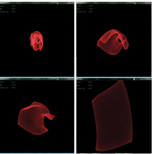
6.9 A screenshot of Velvet capturing the starting positions of 32,768 particles projected inside a 3-ball. This sample is running on an NVIDIA GTX 680 GPU. . . 103

6.10 FDGV running a visualization of a graph with a grid-like structure consisting of 6,400 vertices and 12,640 edges. . . 106

6.11 Comparison of latency vs.eective latency for single GPU performance. . . 119

6.12 Comparison of throughput vs.eective throughput for single GPU perfor-mance. . . 121

6.13 Comparison of the latency and eective latency for GapsMis-drunning on a single GPU device performing alignments allowing 2 gaps. . . 122

6.14 Comparison of the latency and eective latency for GapsMis-drunning on a single GPU device performing alignments allowing 3 gaps. . . 123

(11)

List of Figures x

6.15 Results comparing the latency and eective latency of executing Velvet-d

for all problem sizes (Figure 6.15(a)). Resulting throughput performance is shown in Figure 6.15(b). Here, due to the small data to computation ratio, the communication time between host and compute device is marginal.125

6.16 Comparison of latency vs.eective latency for complete graph (400 ver-tices, 79,800 edges) . . . 126

6.17 Comparison of latency vs.eective latency for Gnutella p2p network graph (26,518 vertices, 65,369 edges) . . . 127

6.18 Comparison of latency vs.eective latency for grid graph (40,000 vertices, 79,500 edges) . . . 128

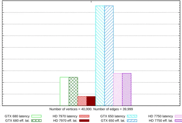
6.19 Comparison of latency vs.eective latency for tree graph (40,000 vertices, 39,999 edges) . . . 129

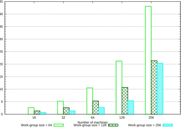
6.20 Latency for DPS-dwith 3,200 jobs with varying work-group sizes on NVIDIA

GTX 680 GPU. . . 130

6.21 Latency for DPS-dwith 3,200 jobs with varying work-group sizes on NVIDIA

GTX 650 GPU. . . 130

6.22 Latency for DPS-dwith 3,200 jobs with varying work-group sizes on AMD

HD 7970 GPU. . . 131

6.23 Latency for DPS-dwith 3,200 jobs with varying work-group sizes on AMD

HD 7750 GPU. . . 131

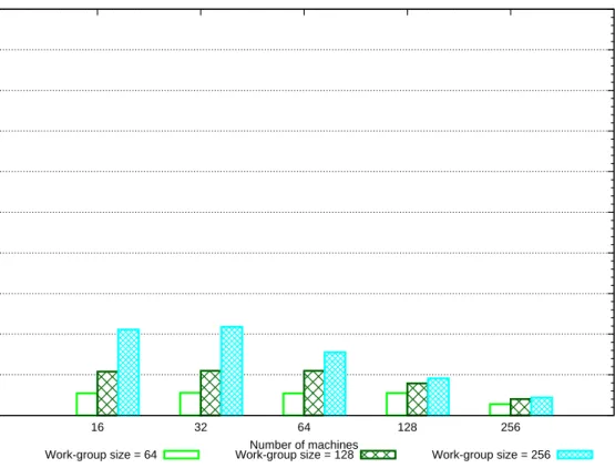
6.24 Throughput for DPS-d with 3,200 jobs with varying work-group sizes on

NVIDIA GTX 680 GPU.. . . 132

AMD HD 7970 GPU.. . . 133

AMD HD 7750 GPU.. . . 133

6.28 Latency for Velvet-dwith varying work-group sizes on NVIDIA GTX 680

GPU. . . 134

6.29 Latency for Velvet-dwith varying work-group sizes on NVIDIA GTX 650

GPU. . . 135

6.30 Latency for Velvet-d with varying work-group sizes on AMD HD 7970

GPU. . . 136

6.31 Latency for Velvet-d with varying work-group sizes on AMD HD 7750

GPU. . . 137

6.32 Results showing the throughput performance of Velvet-das work-group

size varies on the NVIDIA GTX 680 GPU.. . . 138

size varies on the NVIDIA GTX 650 GPU.. . . 139

size varies on the AMD HD 7970 GPU.. . . 140

size varies on the AMD HD 7750 GPU.. . . 141

6.36 Results showing latency performance FDGV-das work-group size varies for

(12)

AMD HD 7970 GPU.. . . 142

AMD HD 7750 GPU.. . . 143

6.40 Results showing throughput performance FDGV-das work-group size varies

for NVIDIA GTX 680 GPU.. . . 143

for NVIDIA GTX 650 GPU.. . . 144

for AMD HD 7970 GPU.. . . 144

for AMD HD 7750 GPU.. . . 145

6.44 Comparison of latency for 1,600 jobs with and without using GPU local memory. . . 145

6.45 Comparison of latency for 3,200 jobs with and without using GPU local memory. . . 146

6.46 Comparison of throughput for 1,600 jobs with and without using GPU local memory. Throughput is measured in millions of cell updates per second (MCUPS).. . . 146

6.47 Comparison of throughput for 3,200 jobs with and without using GPU local memory. Throughput is measured in millions of cell updates per second (MCUPS).. . . 147

6.48 Results showing the eect of local memory on the latency performance of Velvet-d for all GPU devices. The work-group sizes in these results are

1024 for NVIDIA GPUs and 256 for AMD GPUs. . . 148

6.49 Results showing the eect of local memory on the throughput performance of Velvet-d for all GPU devices. The work-group sizes in these results

are 1024 for NVIDIA GPUs and 256 for AMD GPUs. Throughput is measured in billions of oating-point operations per second. . . 149

6.50 Results showing the eect of local memory on latency performance of FDGV-dfor all GPU devices. The work-group sizes in these results are 512

for NVIDIA GPUs and 256 for AMD GPUs. . . 150

6.51 Results showing the eect of local memory on latency performance of FDGV-dfor all GPU devices. The work-group sizes in these results are 512

for NVIDIA GPUs and 256 for AMD GPUs. Throughput is measured in billions of oating-point operations per second. . . 151

6.52 Results showing the benets of using pre-pinned memory for Velvet-d

and FDGV-drunning on our designated reference machine. Time elapsed is

given in microseconds. . . 152

6.53 Results showing the benets of using pre-pinned memory for Velvet-d

and FDGV-drunning on our designated reference machine. Time elapsed is

given in microseconds. . . 153

6.53 Comparison of how GapsMis-dscales with the addition of a second GPU

device. Results shown here are for an alignment that allows 3 gaps. Throughput is measured in billions of cell updates per second (GCUPS) . 160

6.54 Throughput performance comparison of how DPS-d scales with the

addi-tion of a second GPU device for simulaaddi-tion with 1,600 jobs. The work-group size used for these results is 256 for all GPU devices. . . 161

(13)

List of Figures xii

6.55 Throughput performance comparison of how DPS-d scales with the

addi-tion of a second GPU device for simulaaddi-tion with 3,200 jobs. The work-group size used for these results is 256 for all GPU devices. . . 162

6.56 Comparison of how FDGV-d scales with the addition of a second GPU

device. The results for NVIDIA GPUs are obtained using a work-group size of 512 and using local memory. The AMD GPUs use a work-group size of 256 and without using local memory. Throughput is measured in billions of oating-point operations per second. . . 163

6.57 Results of power consumption proling for each application on each device conguration. . . 164

6.58 Latency performance of GapsMis-s vs GapsMis-d on single GPU for a

3-gap alignment. The length of target sequences is 250 and 200 for query sequences. . . 165

6.59 Latency performance of GapsMis-twith 12 CPU threads vs GapsMis-don

dual GPUs for a 3-gap alignment. The length of target sequences is 250 and 200 for query sequences.. . . 166

6.57 Comparison of CPU vs GPU performance of DPS for a problem size con-sisting of 3200 jobs.. . . 169

6.57 Comparison of energy consumption and eciency for CPU and GPU de-vices for DPS. Energy consumption is given in Watt-second while eciency is given in millions of cell updates per second per Watt. . . 171

6.57 (a) Ratio of CPU performance to single GPU performance with respect to latency. (b) Comparison of CPU vs.GPU in terms of eciency measured in billions of oating-point operations per Watt. . . 172

6.57 Comparison of energy consumption for CPU and GPU devices for Velvet. Energy consumption is measured in Watt-second. . . 173

6.57 Comparison of CPU vs.GPU execution times for FDGV. The largest value for each graph is shown in the labels within the plot. . . 175

6.57 Comparison of CPU vs.GPU energy consumption and eciency for FDGV. Energy consumption is measured in Watt-second and eciency is mea-sured in GFLOPS/Watt.. . . 177

A.0 Comparison of the performance ratio based on total ow time plus energy of AJC when using SJF vs. SRPT on a single processor. Inter-arrival times are given by Poisson distribution and job sizes are given by uniform distribution. . . 182

A.0 Comparison of the performance ratio based on total ow time plus en-ergy of AJC when using SJF vs. SRPT on a single processor. Uniform distribution is used for both inter-arrival times and job sizes. . . 184

A.0 Comparison of the performance ratio based on total ow time plus energy of AJC when using SJF vs. SRPT on a single processor. Uniform distribu-tion is used for job sizes while Poisson distribudistribu-tion is used for inter-arrival times. . . 186

A.0 Comparison of the performance ratio based on total ow time plus energy for AJC when using SJF vs. SRPT on 4 processors. Poisson distribution is used for the inter-arrival times while uniform distribution is used for the jobs sizes. . . 189

(14)

A.0 Comparison of the performance ratio based on total ow time plus energy for AJC when using SJF vs. SRPT on 4 processors. Uniform distribution is used for both the inter-arrival times and jobs sizes. . . 191

A.0 Comparison of the performance ratio based on total ow time plus energy for AJC when using SJF vs. SRPT on 4 processors. Uniform distribution is used for the inter-arrival times and Poisson distribution is used for jobs sizes. . . 193

A.0 Eectiveness of speed scaling: Comparison of the performance ratio based on total ow time plus energy between AJC and a xed speed heuristic that uses a xed speed of 1 on a single processor. Poisson distribution is used for inter-arrival times and uniform distribution is used for job sizes. . 196

A.0 Eectiveness of speed scaling: Comparison of the performance ratio based on total ow time plus energy between AJC and a xed speed heuristic that uses a xed speed of 1 on a single processor. Uniform distribution is used for both inter-arrival times and job sizes. . . 198

A.0 Eectiveness of speed scaling: Comparison of the performance ratio based on total ow time plus energy between AJC and a xed speed heuristic that uses a xed speed of 1 on a single processor. Uniform distribution is used inter-arrival times and Poisson distribution is used for job sizes. . . . 200

A.0 Speed scaling vs. semi-clairvoyant xed speed function: Comparison of the performance ratio based on total ow time plus energy between AJC and a xed speed function that has some information about the job set. Poisson distribution is used for inter-arrival times and uniform distribution is used for job sizes. . . 203

A.0 Speed scaling vs. semi-clairvoyant xed speed function: Comparison of the performance ratio based on total ow time plus energy between AJC and a xed speed function that has some information about the job set. Uniform distribution is used for both inter-arrival times and job sizes. . . 205

A.0 Speed scaling vs. semi-clairvoyant xed speed function: Comparison of the performance ratio based on total ow time plus energy between AJC and a xed speed function that has some information about the job set. Uniform distribution is used for inter-arrival times and Poisson distribution is used for job sizes. . . 207

A.0 Eectiveness of AJC speed spectrum: Comparison of AJC to a xed speed function that uses, as xed speed values, the average and maximum speeds obtained from a prior AJC run. Results show the performance ratio of the total ow time plus energy of xed speed functions vs. AJC. Poisson distribution is used for inter-arrival times and uniform distribution is used for job sizes. . . 210

A.0 Eectiveness of AJC speed spectrum: Comparison of AJC to a xed speed function that uses, as xed speed values, the average and maximum speeds obtained from a prior AJC run. Results show the performance ratio of the total ow time plus energy of xed speed functions vs. AJC. Uniform distribution is used for both inter-arrival times and job sizes. . . 212

(15)

List of Figures xiv

A.0 Eectiveness of AJC speed spectrum: Comparison of AJC to a xed speed function that uses, as xed speed values, the average and maximum speeds obtained from a prior AJC run. Results show the performance ratio of the total ow time plus energy of xed speed functions vs. AJC. Uniform distribution is used for inter-arrival times and Poisson distribution is used for job sizes. . . 214

A.-2 Results on processor allocation strategies in terms of average job size: Fig-ures A.1(a) to A.1(d) show the performance ratios for average job size of 1. Results for average sizes of 16 and 512 are shown in Figures A.0(g), A.0(h), A.1(e) and A.1(f) and Figures A.-1(j) to A.-1(l) and A.0(i) re-spectively. Results measure the performance ratio of total ow time plus energy for a single processor vs. multiple processors. Poisson distribution is used for inter-arrival times and uniform distribution is used for job sizes.219

A.-4 Results on processor allocation strategies in terms of average job size: Fig-ures A.-1(a) to A.-1(d) show the performance ratios for average job size of 1. Results for average sizes of 16 and 512 are shown in Figures A.-2(g), A.-2(h), A.-1(e) and A.-1(f) and Figures A.-3(j) to A.-3(l) and A.-2(i) re-spectively. Results measure the performance ratio of total ow time plus energy for a single processor vs. multiple processors. Uniform distribution is used for both inter-arrival times and job sizes. . . 223

A.-6 Results on processor allocation strategies in terms of average job size: Fig-ures A.-3(a) to A.-3(d) show the performance ratios for average job size of 1. Results for average sizes of 16 and 512 are shown in Figures A.-4(g), A.-4(h), A.-3(e) and A.-3(f) and Figures A.-5(j) to A.-5(l) and A.-4(i) re-spectively. Results measure the performance ratio of total ow time plus energy for a single processor vs. multiple processors. Uniform distribution is used for inter-arrival times and Poisson distribution is used for job sizes.227

(16)

List of Tables

3.1 Lookup tables showing processing and communication costs with respect to time and energy. . . 31

3.2 Dynamic programming table for job J1 in the problem described in

Ex-ample 3.1. . . 32

3.3 Solution for the dynamic programming table for the problem described in Example 3.1. . . 33

3.4 Solution for the dynamic programming table for the problem described in Example 3.1 without the redundant values. . . 33

4.1 Summary of the best performance ratios for all processor allocation strate-gies. . . 58

6.1 Table listing hardware specications of all host systems used in the exper-iments.. . . 111

6.2 Intervals used in data generation for DPS. These intervals are inclusive in the resulting data. . . 112

6.3 Information for GenBank databases used to generate input sequences for GapsMis.. . . 114

6.4 Details of the real graph data obtained from SNAP.. . . 114

6.5 Details of the synthetic graph data generated for FDGV application. . . 115

(17)

Dedicated to my family, for providing me with the means to pursue

my dreams. And to my supervisor, Dr. Prudence Wong, for making

those dreams a reality.

(18)

Introduction

1.1 Overview

The study of scheduling dates back as far as the 1950s when researchers in operations research, industrial engineering and management were faced with the problem of

manag-ing various activities occurrmanag-ing in a workshop [64]. An organization can lower production

costs in its manufacturing processes thereby enabling it to stay competitive. Later on in the 1960s computer scientists also encountered scheduling problems during the develop-ment of operating systems. During this time period computer resources such as CPU, memory and I/O devices were considerably scarce so it was crucial that they had to be eciently utilized in order to minimize the cost of running these computer systems. Therefore an economic reason to study scheduling was established and eventually vari-ous classes of scheduling problems have been developed to take into account the dierent scenarios they aim to address. Even in present times, new scheduling problems arise from various sources such as the introduction of a new technology in various elds like systems design, automated industrial processes and so on.

Advances in the technology of microprocessor development and chip fabrication process means that the density of transistors that make up these chips continue to grow. In addition, the computational power and processing capability of these chips somewhat doubled with each new design as manufacturers are able to ramp up the clock speeds with the introduction of subsequent generations of microprocessors. Consequently, operating at high clock speeds usually comes at the expense of incurring exponential increase in power consumption and in order to mitigate this issue, manufacturers resorted to shrinking chip sizes but this process has been restricted by available technology. As

a result, the growth in clock speeds began to slow down [103] and the gains in the

performance levels of these chips began to diminish. Chip manufacturers pursued other 1

(19)

Chapter 1. Introduction 2 means of achieving higher performance and this brought about the advent of multi-core technology and mainstream parallel computation. Multi-multi-core processor technology was particularly attractive and promising especially because manufacturers were able to more than double performance without necessarily increasing the operating frequency by simply adding more processing cores. This means that devices are able to do more as more processing power became readily available and this lead to an age of ubiquitous computing as these chips powered almost everything ranging from small devices such as mobile phones and tablets to our home computers to enterprise server systems and super-computers. However, the problem of energy consumption soon re-surfaced and it became highly imperative that system designers and developers tackle the issue for both technical and economic reasons in order to prolong the sustainability of multi-core and parallel systems.

On the economic side, apart from the costs of powering these computer systems, ex-tra costs are incurred as a result of cooling systems required to keep them within their optimal operating conditions. Since signicant amount of the energy drawn by these sys-tems is dissipated as heat, the life span of a system can be greatly shortened due to the adverse eects of high temperatures such as degraded transistor performance and dam-age to components like soldering which can cause permanent damdam-ages. Therefore, the problem of managing energy has become a critical topic in both industrial and academic research and various approaches have been considered leading to innovations in algorithm designs, software and hardware. Among the several approaches of managing energy con-sumption, a growing trend is the adoption of heterogeneous computing to deliver high performance. This is evident from the recent rankings of the 500 most powerful and

energy-ecient supercomputers where the 17 most energy-ecient supercomputers [38]

as well as the most powerful supercomputer [106] are heterogeneous systems utilizing

graphics processing units (GPU) and other co-processors.

The development of heterogeneous and parallel systems oer exciting prospects in the quest to nd a balance between energy consumption and performance of computer sys-tems. The GPU has shot to the forefront as most used co-processor in heterogeneous systems quite simply because it was already part of existing systems where it is used for visual and rendering tasks making its adoption very easy. As a part of this thesis, we will present a detailed study to demonstrate the benets of a heterogeneous system that includes the GPU with respect to saving energy while achieving high computational performance.

This chapter is organized as follows; in Section1.2, we discuss some of the basic concepts

(20)

introduced in Section 1.3. Finally, in Section 1.4, we outline the contribution of the thesis.

1.2 Background on Scheduling

Scheduling can be generally considered as dealing with allocation concerns involving scarce resources and tasks or operations that demand them with the goal of optimizing one or more performance measures of interest in a given setting. These resources could refer to a number of entities depending on the situation being considered. These may include cores in a multi-core CPU, CPUs in a multiprocessor system, servers in a server farm or cluster, memory, I/O devices, machines in an assembly line, airport runways, train stations, personnel assignment in workplaces, just to mention a few. Operations, on the other hand, may also refer to train calls at stations, airport landing and take-os, an operation in a manufacturing process, execution of a computer program, manning workstations in an industrial setting or call centres.

1.2.1 Inputs and outputs

The inputs in a scheduling problem includes a set consisting of a number of jobs to be executed on a set consisting of a number of machines and each job or machine can be uniquely referenced by a subscript. The time at which a job becomes available for

processing is known as the release or arrival time. The time it takes for a job j to

completely execute on a machine i is known as its processing time, and this value is

assumed to be nite and non-negative unless explicitly stated. The point in time at which

jobjnishes its execution is known as its completion time. In some cases a job is required

to nish execution at a particular time or deadline, however, a job might nish at a time greater than the time specied as its deadline. The term tardiness measures how late a

job completes past its deadline and is expressed as max{completion time−deadline, 0},

while earliness, expressed as max{deadline−completion time, 0}, measures how much

a job completes before its deadline. Hence, when a job completes before its deadline its tardiness is 0, and when a job completes after its deadline then its earliness is 0.

In order to represent each scheduling problem in a concise way including the inputs, constraints and objective function(s), I would like to mention the well-known three-eld

α|β|γ notation rst introduced by Graham et al. [35]. However, we will be describing the

(21)

Chapter 1. Introduction 4

1.2.2 The α|β|γ scheduling notation

The rst eld α = α1α2α3 in the notation describes the machine environment in a

problem setting. Parameterα1{∅, P, Q, R, F, J, O} is used to characterize the machines

in single machine, identical, uniform and unrelated parallel machines, ow shop, job

shop and open shop problem settings respectively. Parameter α2{∅, m}, where m is a

positive integer, indicates that the number of machines in a parallel machine environment

or number of stages for dedicated machines is assumed to be the variablem. Parameter

α3{∅, hi,k} describes unavailability intervals which occur on the machines otherwise

referred to as holes. In this notation α =∅ represents a problem setting with no holes

andhi,k species the number of holes and the machine(s) on which they occur. However

α=hi,k represents a problem setting with an arbitrary number of holes on each machine.

If i is replaced by a positive integer it means that holes only occur on machine Mi

otherwise holes will occur on all machines but if k is replaced by a positive integer it

denotes the number of holes occurring on the corresponding machine. For instance,

α = h1,k denotes a problem with an arbitrary number of holes on M1 only; α = hi,1

represents a problem with one hole on each machine whileα=h1,1 represents a problem

with one hole on machine M1 only.

The second eld β = β1, ..., β5 describes characteristics or constraints associated with

operations (jobs) and resources. Parameter β1{∅, t−pmtn, pmtn} denotes the kind of

preemption constraint in place which is either non-preemption, operation preemption or arbitrary preemption respectively. An operation is said to be preempted if its processing on a particular machine is interrupted at any time and resumed later at any time and restarted at no cost. It must either remain on the same machine until it can be continued later (operation preemption) or it can be shifted to another machine (arbitrary

preemp-tion). However, there are several studies that useβ1 =r−a,β1=nr−aand β1 =sr−a

to represent resumable, non-resumable and semi-resumable availability constraints

re-spectively [68]. In the resumable case preemption is allowed so if an operation cannot

be completed before the unavailability period of a machine it can resume later when the machine becomes available again. The non-resumable case does not allow preemption so the disrupted operation has to completely restart instead of continue. However, in the semi-resumable case, operations can only be restarted partially after the machine

be-comes available again. Parameterβ2{∅, rj}indicates release time for operations (jobs),

which can either be zero or dier respectively. Parameter β3{∅, dj} denotes deadline

constraints on the job set where β3 = ∅ indicates no assumed deadlines, however, due

dates may be dened if necessary. On the other hand, β3 = dj indicates a deadline

constraint imposed in the job set. Parameter β4{∅, qj} indicates the absence or

(22)

problem is said to be oine if we have full knowledge regarding job data before building a schedule or online if a scheduling decision is required once a job arrives without any

information about jobs that are yet to arrive in the future [68]. The β eld can also

be left blank to denote no constraints on the job set and that all the jobs are available before the construction of the schedule begins.

The third eld γ represents the performance measure or objective function to be

opti-mized. Some of the commonly studied objective functions include maximum completion

time of all jobs or makespan (Cmax), minimum completion time (Cmin), maximum

late-ness (Lmax), maximum tardiness (Tmax), total completion time (PCi), total weighted

completion time (P

wiCi), number of tardy jobs (P

Ui) and weighted number of tardy

jobs (P

wiUi).

1.2.3 Classes of scheduling problems

Single machine problems.

The single machine problem simply involves scheduling a set of jobs on one machine only which can either be assumed to be continuously available throughout the processing period of the job set or have periods of unavailability or holes. It is the simplest form of the scheduling problems.

Parallel machine problems.

The parallel machines can be further subdivided into identical (Pm), uniform (Qm) and

unrelated(Rm)parallel machines. The variablemusually indicates the number of parallel

machines in the problem setting which can also be omitted to denote an arbitrary number of machines. Identical parallel machine problem involves a set of identical machines running at the same speed, therefore, a given job will take the same amount of time to process on all the machines. For the case of uniform parallel machines each machine

runs at a dierent speed. For instance machine Mi, 1≤ i≤m, runs at speedsi. The

processing timepij that jobJj spends onMi is given bypj/si assumingJj is completely

processed by Mi. Finally, in unrelated parallel machines, the jobs are processed at

dierent speeds on the machines so even if two machines run at the same speed it does not necessarily mean that they will take the same amount of time to process a particular job.

Job shop problems (Jm).

In this problem setting withmmachines there is a set ofnjobs that need to be processed

(23)

Chapter 1. Introduction 6 predetermined route through the machines so a job can use some machines more than once and may not use some machines at all. For instance, in a problem consisting of

m=10machines labelled seriallyM1, ..., M10, a jobJj might have a predetermined route

through machines M1,M3,M5 and M1 exactly in that order. The order in which a job

executes must follow the order in the predetermined route.

Flow shop problems (Fm).

Here allm machines are ordered linearly and all the jobs in the job set must follow the

same route from the rst machine to the last machine in order to be processed.

Open shop problems (Om).

In an open shop problem of m machines alln jobs in the job set needs to visit each of

the machines at least once and the order in which this happens is not relevant.

1.2.4 Input structure and constraints

Apart from the machines a certain structure or constraint can exist in the set of jobs to be processed known as precedence constraints. This could be in the form of an intree, outtree

or chain. Precedence constraints are specied explicitly in theβ eld or generally written

as precand it is always given as a directed acyclic graph where each vertex represents

a job. Job iprecedes job j if there is a directed arc from ito j meaning that imust be

completed beforejstarts. A chain exists when each job has at most one predecessor and

at most one successor. An intree is such that each job has at most one successor while an outtree is when each job has at most one predecessor. It also possible to restrict the

number of jobs by including the symbolnbrin theβ eld which is the maximum number

of jobs to be processed. For ow shop problems only a no-wait constraint (nwt) can be

specied to denote that jobs are not allowed to wait between two successive machines.

Also a restriction can be imposed on the processing time of the jobs using pj = p in

the β eld to denote that each job's processing time is p units. Finally, in job shop

problems where jobs can have operations, the sub-eld nj is used to restrict the number

of operations allowed for each job.

1.3 Problems Studied and related work

1.3.1 Online scheduling of deteriorating jobs on parallel machines

In classical scheduling problems, it is usually of the assumption that the processing of jobs are xed, however, this is not always the case in some practical situations. There

(24)

are various scenarios where the processing time of a job increases of deteriorates as the start time increases or is delayed. An instance of this scenario would be in the continuous casting stage in a steel production process. This requires that the steel is still in molten form in order to be cast into slabs, blooms or billets. Any delays in the prior processes might result in the steel cooling down to unacceptable temperatures which may result in a restart in the whole process, leading to additional time as a consequence. Other examples can be found in re-ghting, cleaning, maintenance tasks and nancial

management [53, 74]. In general, any delay in the start time of such task would incur

additional eort to complete it at a later time, hence, the reason and motivation behind the study of deteriorating jobs.

The problem of scheduling deteriorating jobs was rst introduced by Gupta and Gupta [41],

and Brown and Yechiali [17]. Although both works studied makespan minimization on

a single machine, the processing time of a job is given as a monotone linear function of its start time in [17] while in [41], it is given as a non-linear function. The problem has since attracted huge interests and has been studied in other time-dependent models with other objective functions [5,24,34].

Linear deterioration. The problem of scheduling jobs with linear deterioration has been studied in great details as a result of its simplicity while capturing the vital prop-erties of practical situations. The processing time of a job is expressed as a monotone

linear function of its start time. To be precise, the processing time pj of a job Jj is

dened as pj =aj+bjsj, where aj > 0 is the normal or basic processing time, bj > 0

is the deteriorating rate and sj > 0 is the start time. As the start time of a job gets

larger, the processing time also gets larger and therefore, the processing time of a job is dependent on the schedule. Furthermore, linear deterioration is said to be simple if

aj = 0, that is,pj =bjsj.

Figure 1.1: An illustration of linear deterioration.

Consider the illustration in Figure 1.1 that shows two jobs, Jj and Jk, with identical

deteriorating rates of 2 scheduled at dierent times. Assume thatt0 = 1andJj starts at

(25)

Chapter 1. Introduction 8 is started later at time 2t0, therefore, the completion time is given by2t0+bk2t0 which

evaluates to 6.

As the number of jobs grows, the start time of jobs gets larger and the processing time of innitely many jobs is no longer aected by the normal processing time but only by

the deteriorating rate [73,74]. In addition, Gupta and Gupta [41] observed that in the

case of linear deterioration, it is optimal to process jobs in ascending order of aj

bj. From this example, we can see that even though both jobs have identical deteriorating rates, their processing times dier signicantly and this demonstrates how the schedule of a deteriorating job can greatly aect its processing time.

Scheduling jobs with linear deterioration has been studied in the contexts of both single machine [74, 80] and parallel machines [33,49,51,75, 92]. In [80], Ng et al presents a study of the problem on a single machine where preemption is allowed and each job is associated with a release time. They show that minimizing the maximum job completion cost is polynomial time solvable whether or not precedence constraints are imposed on the jobs. They also show that minimizing the total weighted completion time is NP-hard

even with only two distinct release times. On parallel machines, Garey and Johnson [33]

showed that the problem is NP-hard for two machines and strongly NP-hard for arbitrary number of machines as a result of the complexity of the corresponding problems with

xed processing time. A FPTAS is proposed by Kang and Ng [49]. For the case of simple

linear deterioration, the problem has been independently shown to be NP-hard [51,75]

and a FPTAS is proposed by Ren and Kang in [92].

Other time-dependent models. In the denition of linear deterioration, pj = aj +

bjsj, bj is assumed to be non-negative and non-decreasing. However, in a dierent

model, bj is assumed to be a non-positive and non-increasing factor. In other words, the

processing time of each job decreases as its start time increases. This model was initiated

in [43] and represents a real-world problem in the military domain where the objective

is to eliminate an aerial threat target. In this case the execution time decreases as the target gets closer.

Another time-dependent model involves scheduling with procrastination. In [15] the

scheduler is assumed to execute a job with increasing speed as the deadline approaches. This models a number of real-world scenarios, most especially human behaviour, where one would postpone execution of an arduous task close to the deadline in order to spend as little time as possible. Another example is the addition of more resources or people to a project in order to meet the project's deadline. For this problem, an optimal oine algorithm was presented for case where a feasible schedule or solution exists. They

(26)

maximum interval stretch, that is, the time allowed for the procrastinator to nish a job beyond its due date.

Online models. Most of the results discussed above assume that the all jobs are

available at the same time so an algorithm has full knowledge (that is, aj and bj) of the

all jobs in advance. However, the reality is that jobs may also have arbitrary release

times. Pruhs et al [91] formalized two online models, namely, online-list and online-time

models. In the online-list model, jobs are released only one at a time so an algorithm must schedule the released job before further subsequent jobs can be released. Once a job is scheduled by the algorithm it cannot be modied in the future. One the other hand, in the online-time model, an arbitrary release time is associated with each job so the information relating to each individual job is only available after it has been released.

Graham [36] proposed a List Scheduling (LS) algorithm for online parallel machine

scheduling with xed processing time. Online algorithms for linear deteriorating jobs with release times have been studied in [23,60]. In [60], the application of deteriorating

jobs with release times to steel production is discussed. Cheng and Ding [23] showed

that the problem with release times on a single machine is strongly NP-hard for the case

of identical normal processing time aor deteriorating rateb.

To the best of our knowledge, the only work on online scheduling of deteriorating jobs

that we are aware of is by Cheng and Sun [22]. In this thesis, we present results in

both contexts of online-list and online-time models for simple linear deteriorating jobs on parallel machines.

1.3.2 Energy-ecient scheduling of precedence-constrained jobs on par-allel machines

In Section 1.3.1, we introduce a scheduling problem with no constraints present in the

structure of the jobs, in other words, each job can be treated as a completely independent entity. However, there are practical situations where the execution of an operation or collection of operations can depend on some factors related to the problem domain. Some of these factors include storage, transportation, resource availability and maintenance, and process constraints which is related to a particular order in which operations must be fullled. A simple example can be found in queueing systems which are applicable to nancial institutions, health care and service industries, where requests are fullled in the order of their arrivals so that earlier ones nish rst. Other examples include automated processes in industrial assembly and fabrication systems in which some operations cannot be carried out without some prerequisite operation, for example, spray-painting process of a car in a vehicle assembly plant cannot begin without rst assembling all vehicle parts.

(27)

Chapter 1. Introduction 10 These kind of restrictions in the scheduling process gave rise to the research and study of scheduling subject to constraints, a class of which consists of precedence constraints. The concept of precedence constraints was introduced to capture the essence of scheduling where operations are not totally independent of each other. In simple terms, precedence constraints specify that a job cannot be started unless all the jobs preceding it have been completed. The precedence constraints between jobs is usually depicted with the

use of a directed acyclic graph. Figure 1.2 illustrates the dierent types of precedence

constraints.

(a) Chain (b) Intree (c) Outtree

Figure 1.2: Examples of job precedence constraints.

The study of scheduling with precedence constraints began as early as 1970s with notable theoretical studies including [58,61,99]. Lenstra and Rinnooy Kan [61] were able to show that most of the relatively simple, classic scheduling problems become NP-complete when precedence constraints are added to these problems.

In this thesis, we present a study of the scheduling of jobs with chain precedence con-straint on parallel machines with the objective of minimizing energy. Our motivation is two-fold. First we present an algorithm for solving the problem, and secondly, our goal is to use our algorithm as a case study in our study involving heterogeneous and parallel computing. The study of energy-aware scheduling on parallel machines or chip multi-processors have received numerous attention in research, however, we are concerned with problems involving non-independent tasks. Some closely related works in this aspect

in-clude [14,97]. Here, tasks are represented as directed acyclic graphs (DAG) where nodes

represent the task while the edges represent the precedence between tasks. The cost associated with processing time and energy as well as communication time and energy are also given as input to the problem. We present a problem using similar model to the works mentioned but our focus in a task set with chain precedence constraint and each task can have a dierent deadline. We present both theoretical results and empirical results for this problem.

1.3.3 Energy-ecient ow time scheduling

Single processor scheduling. The theoretical study of dynamic speed scaling to

(28)

of attention [16,26,88]. Yao et al. considered the innite speed model where a processor can dynamically change its speed to a value between zero and innity. They studied the problem of online scheduling of jobs with arbitrary sizes and deadlines, and their objective is to produce a schedule such that all jobs complete within their deadline while minimizing the energy incurred by the schedule. The study has been extended to take into consideration the fact that in realistic situations processors can only adjust speeds within a nite speed spectrum with often pre-dened voltage levels. Here, processor voltage is determined from a nite spectrum of discrete voltage levels which in turn determines the speed levels the processor is capable of running at. Earlier approaches to the problem involve rst computing the continuous version of the problem and then adjusting the speeds to the t into the discrete voltage levels for the nal schedule [47,56].

Yao and Li [65] further extended the study and presented results where the computation

of the continuous schedule is skipped entirely.

On the other hand, the problem of minimizing total ow time plus energy compacted into a single objective function dened as the sum of ow time and energy was proposed

by Albers and Fujiwara [4]. They considered jobs of unit size and propose a speed scaling

algorithm that changes the speed of the processor based on the number of active jobs (AJC), which refers to jobs that have arrived but are yet to be completed. They, however, studied a batched version of the algorithm where newly released jobs are queued until all

jobs in the current batch are completed and showed that it is8.3e(1 + Φ)α-competitive

for minimizing total ow time plus energy, whereΦ = (1+

√

5)

2 is the golden ratio. Further

improvement on their work has been presented by Bansal et al. [11,12].

Multiple processor scheduling. The problem of scheduling on multiple processors

with xed speed and without energy considerations has been widely studied [8, 9, 19,

20,62]. The use of multiple processors can be seen in practice in most modern computer

systems and devices where the most common conguration consists of identical processing cores, for instance, processors found in home desktop machines and most recently, mobile phones and tablets. For the problem involving multiple processors, jobs still arrive in a sequential fashion and cannot be executed by more than one processor in parallel. Online algorithms such as shortest remaining processing time (SRPT) and immediate

dispatch (IMD) [8] that are Θ(log P)-competitive have been proposed for the migratory

and non-migratory model respectively, whereP is the ratio of the maximum job size to

the minimum job size [8, 9, 62]. Furthermore, IMD has been shown to be O(1 + 1)

-competitive when using processors that are (1 +) times faster. In the case where

migration is allowed, SRPT has been to achieve a competitive ratio of 1 or even smaller

(29)

Subsequently, Bunde [18] initiated the study of multiple processor scheduling that takes

both ow time and energy into account and presented a study of the oine approximation

for jobs with unit size. On the other hand, Lam et al. [57] presented the rst online,

non-migratory algorithm for minimizing total ow time plus energy for jobs of arbitrary size. Conserving energy with multiple processors typically involves distributing jobs as evenly as possible among the available processors in order to avoid running any processor at higher than required speed, therefore, it is only natural to consider techniques similar

to round-robin. This is demonstrated by Lam et al [57] in the classied round robin

(CRR) algorithm, which classies jobs according to their sizes and allocates jobs of the same class to the processors in a round robin fashion. They showed that CRR can be Θ(log P)-competitive for the problem of minimizing total ow time plus energy.

In this thesis, we present an empirical study that focuses on the analysis of the speed-scaling heuristic based on the number of active jobs and investigate the possibility of designing a simpler heuristic that is capable of achieving the sort of performance close to that of the speed-scaling heuristic. In addition, our investigation includes several speed selection, job selection and multi-processor allocation heuristics.

1.3.4 Parallel and heterogeneous computing with graphics processors

Over the years, chip manufacturers have greatly concentrated on improving single-thread performance of the central processing unit (CPU), which provides the bulk of the comput-ing power in enterprise and home computer systems. However, the future of computcomput-ing centres around parallelism and heterogeneous computing. As it is the current trend, the design and development of future microprocessors will continue to focus adding more computing cores instead of simply focusing on single-thread performance or frequency. The Cell broadband engine. One of the earlier trends in heterogeneous computing

involves the use of the Cell broadband engine [69]. The Cell processor was developed by

Sony, Toshiba and IBM and it provides the processing power for the Sony Playstation 3 game console. The heterogeneous nature and multicore architecture quickly attracted attention in the science and research communities. A number of the initial works such as [10,21,54,55,108] focused on using the Cell processor to accelerate scientic compu-tations including 1D/2D Fast Fourier Transforms, and several linear algebra techniques including QR factorization, Cholesky factorization, dense matrix operations and sparse matrix-vector operations. These results show that using the Cell processor for these applications resulted in signicant performance increase compared to the conventional CPUs available during the same period.

(30)

GPU computing. Another kind of multiprocessor that quickly gained popularity among the scientic community is the graphics processing unit (GPU). The GPU is a multiprocessor primarily designed to accelerate compute tasks involved in graphics rendering. It is specically designed for high throughput computation rather than low latency computation as is seen with the CPU. It is also optimized to handle compute tasks that require high levels of parallelism as is associated with rendering of pixels and other graphics-related tasks. Due to these reasons, the GPU is characterized by a mas-sively parallel architecture with hundreds of processing elements. In addition, the GPU is readily available and the desktop versions can be very aordable. These factors make it very appealing to the scientic community, hence, the signicant amount of attention it has received over the years. The use of graphics processors for accelerating applica-tions is commonly referred to as GPU computing or general purpose computing on GPUs

(GPGPU). Owens et al. provides a comprehensive survey and introduction in [85,86].

GPU computing has seen applications in several elds. In Computer Science, there has been several work in literature that study the implementation of several algorithms on the GPU and evaluate their performance. Problems in graph theory including graph

cuts, traversal and layout have already been studied in [31, 42, 72, 107]. Furthermore,

sorting algorithms including merge sort, radix sort, quick sort and bitonic sort, just to

mention a few, have been analysed on the GPU [37,39,94,96,100].

Another eld of study where GPU computing has received a lot of attention is Bioin-formatics. Some of the applications used in Bioinformatics are typically characterized as mainly requiring high throughput computation. Therefore, it is no surprise that the graphics processor has been adopted to accelerate the performance of such appli-cations. GPU computing is applied to applications used for sequencing, alignment and database searches and some the works include implementation of the very popular Smith-Waterman algorithm [101] on the GPU [67], and tools such as [66,98,113,114]. Majority of the works provided by the authors relating to GPU computing are accompanied with empirical studies demonstrating the advantages that the GPU oers over conventional computing with CPUs.

In this thesis, we are not only interested in presenting new implementations of algorithms on the GPU. We will be presenting a study detailing our experiences in developing applications on the GPU. We will study several factors that can easily be overlooked when designing applications for GPGPU which are key in order to achieve desired levels of performance on the GPU. In order to do this, we will select a few algorithms as representative case studies. Some of which are already known algorithms but have not been studied in the context of GPU computing, at least to the best of our knowledge, and others will be a novel approach.

(31)

1.4 Contribution of thesis

In Chapter2 of this thesis, we present a theoretical study of the problem of scheduling

linear deteriorating jobs on parallel machines with the objective of minimizing makespan. This is a joint work with Sheng Yu, Prudence Wong and Yinfeng Xu, and is published

in the Theory and Applications of Models of Computation [112]. We present three main

results in the online-time model, where jobs are associated with arbitrary release times. Our rst result concerns the List Scheduling (LS) on arbitrary number of parallel

ma-chines in which we show that the competitive ratio of LS is at least (1 +bmax). We

present details of the adversary as well as mathematical proof for the adversary used to obtain this competitive ratio. The second result concerns the scheduling of simple linear deteriorating jobs on arbitrary number of machines. We show that no

determin-istic algorithm is better than (1 +bmax)1−m1 -competitive and that this also holds for

the online-list model. Finally we extend our adversary to show that in the case of two-machine scheduling of jobs with simple linear deteriorating rates, no deterministic online

algorithm is better than (1 +bmax)-competitive.

In Chapter 3, we present a study of a problem concerned with energy-aware scheduling

of ntasks with precedence constraints on m parallel machines. The type of precedence

constraints we focus on is the chain precedence constraint, where each task can have at most one predecessor and at most one successor. A task is also characterized by a strict deadline that must be met. The parallel machines are assumed to be unrelated and are connected by an underlying communication network. The execution of a task on a machine costs time and energy and for each machine-job pair, the cost is given by a machine-job matrix. Similarly, communication across the network costs time and energy too given in a machine-machine cost matrix. We assume that the communication links can be asymmetric, that is, the cost depends on the direction between a pair of machines. We present an optimal, pseudo polynomial algorithm using a dynamic

programming approach with a running time of O(nm2dmax), where dmax is the largest

deadline. In addition, we implement this algorithm in our empirical studies involving multi-core processors and graphics processors. The aim is to provide a representative case for serial, monadic dynamic programming formulations for analysis on the GPU.

In Chapter 4, we present a study of the problem of scheduling to minimizing total ow

time plus energy. Results of our work was presented at the 11th Workshop on Models and

Algorithms for Planning and Scheduling Problems, 2013 [83]. Our contribution to the

problem is a comprehensive empirical study that aims to complement results obtained from theoretical studies. We implement and investigate several job selection, speed func-tion and processor allocafunc-tion heuristics. We start by considering SRPT and shortest