DOCUMENT DE TREBALL
XREAP2010-1
The Accessibility City.
When Transport Infrastructure Matters in
Urban Spatial Structure
The Accessibility City.
When Transport Infrastructure Matters in
Urban Spatial Structure
Miquel- `Angel Garcia-L´opez
GEAP-XREAP
Department of Applied Economics Universitat Aut`onoma de Barcelona
Abstract
Suburbanization is changing the urban spatial structure and less monocen-tric metropolitan regions are becoming the new urban reality. Focused only on centers, most works have studied these spatial changes neglecting the role of transport infrastructure and its related location model, the “accessibility city”, in which employment and population concentrate in low-density set-tlements and close to transport infrastructure. For the case of Barcelona, we consider this location model and study the population spatial structure between 1991 and 2006. The results reveal a mix between polycentricity and the accessibility city, with movements away from the main centers, but close to the transport infrastructure.
Key words: Urban Spatial Structure, Suburbanization, Decentralization, Transport Infrastructure, Location and Land Use Patterns
1. Introduction
At the present time, most large cities in the World are undergoing a pro-cess of employment and population decentralization-suburbanization that is changing their urban spatial structures. Main centers are losing employ-ment and population in favour of peripheral locations. Furthermore, they are losing influence on the location and land consumption patterns in the non-central areas. As a result, less monocentric metropolitans regions are
becoming the new urban reality (Anas et al., 1998; Giuliano and Redfearn, 2007; Cox et al., 2008).
Theoretical and empirical works have studied these spatial changes fo-cusing their attention on centers, the former explaining the main factors influencing their emergence and decline and the transition between urban forms (Ogawa and Fujita, 1980; Fujita and Ogawa, 1982), the latter pro-viding methodologies for their identification and classifying cities as mono-centric, polycentric and dispersed (Giuliano and Small, 1991; Gordon and Richardson, 1996; McMillen, 2001). As a whole, these studies have neglected the location role of transport infrastructure or, at least, included it into the abovementioned spatial configurations (White, 1976; Steen, 1986; Sullivan, 1986).
From our point of view, employment and population are spatially orga-nized not only around main centers, but also around transport infrastructure. In the case of employment, because it provides better access to agglomera-tion economies, workers, customers or suppliers, etc., and, in the case of population, because it improves accessibility to employment, consumption, amenities, etc. In this context, locations close to freeways, ramps, railroads and stations, among others, might become density maxima from where the rest of the employment and population structure their location and land consumption patterns in a decreasing way, that is, with density falling as firms and individuals move away from transport infrastructure. This spatial pattern is what we call the “accessibility city”.
For the case of the Barcelona Metropolitan Region (BMR), we study the location and land consumption patterns of population and their evolu-tion between 1991 and 2006. The goal is to provide some insight into the location model discussion by taking into account the role of the transport infrastructure and, therefore, considering the accessibility model as an al-ternative spatial configuration. Furthermore, considering different types of transport infrastructures (limited access freeways, free access main roads, ramps, railroads and stations) , we also study different types of accessibility models.
The paper begins by summarizing the standard characterization of trans-port infrastructure in theoretical works where monocentricity, polycentricity and/or dispersion are the only urban forms studied, but also a few other models where transport infrastructure is taken into account in a more real-istic way and our proposal to consider the accessibility city as an alternative spatial configuration. Moreover, Section 2 also shows how empirical
litera-ture has only focused on main centers providing and/or using identification methodologies to deal with the urban spatial structure discussion, but with-out paying attention to the accessibility model. Section 3 introduces the Barcelona Metropolitan Region during the 1991-2006 period, the available data and the main features of its urban spatial structure, applying one of the usual methodologies, and its transport infrastructure. In Section 4 we present our empirical approach to study the BMR’s spatial structure and its evolution considering the accessibility city as another location model besides polycentricity and dispersion. The empirical results are discussed in Section 5. Finally, the main conclusions of the study are outlined.
2. Transport Infrastructure and Urban Spatial Structure
2.1. Theoretical Studies
2.1.1. The Standard Point of View
From a theoretical point of view, the role of transport infrastructure on urban spatial structure has been studied in the context of the Bid Rent Model reformulated based on the New Urban Economics (NUE). The standard point of view departs from the seminal works of the NUE, Alonso (1964), Mills (1967) and Muth (1969), and consider a non-limited radial-type transport infrastructure covering the whole city in the same way and therefore allowing the same access to the CBD from any point located at the same distance from this center. The way transport infrastructure is modelized leads to a
homogeneous reduction in the density as population and employment1
move away from the CBD (a CBD gradient). In this spatial structure, commonly called the monocentric model, the decentralization-suburbanization process reduces central densities and increases peripheral ones, being the resulting spatial structure more dispersed than the previous one.
Following the mid-seventies, the so-called non-monocentric/polycentric
NUE models2
appeared allowing the possibility of other different spatial con-figurations besides the monocentric form. In this sense, considering linear cities or adapting the transport infrastructure standard point of view to the possibility of more centers, that is, a transport infrastructure system that
1
As it is shown by McDonald and Prather (1994) and McDonald (1997). 2
See White (1999) for an excellent review of non-monocentric/polycentric models and their main characteristics.
provides the same accessibility level to the other centers from any point lo-cated at the same distance to these other centers, works such as Ogawa and Fujita (1980), Fujita and Ogawa (1982), Ogawa and Fujita (1989) or Lu-cas and Rossi-Hansberg (2002), among others, analyze the conditions that explain the emergence of monocentric, polycentric and dispersed cities. 2.1.2. A More Realistic Point of View
Although the abovementioned treatment of the transport infrastructure is the “standard” in the NUE literature, there are a few theoretical models that consider the role of this infrastructure on the urban spatial structure in a more realistic way. In this sense, close to the NUE seminals works and therefore based on a monocentric spatial structure, Steen (1986) develops a model which explains how population decentralization-suburbanization ben-efits locations close to transport infrastructure (the railroad system). This infrastructure, although being radial, no longer applies to the whole city; instead, it benefits only certain zones of the metropolitan region, the ones where railroad lines are located. These locations show better accessibility than the others, making them more attractive for population and employ-ment and encouraging their concentration there. In this case, as well as the fall in densities from the center (CBD gradient), which now is not ho-mogeneous for areas located at the same distance, the decrease in densities
occurring from the transport infrastructure must be added3
(a infrastructure gradient). In this model, the decentralization-suburbanization process ben-efits non-central locations near the transport infrastructure, thereby leading to an increase in its structuring role (in the infrastructure gradient).
Used to explain the emergence of a polycentric spatial structure, the non-monocentric NUE models by White (1976) and Sullivan (1986) consider a circumferential transport infrastructure (freeway). In White (1976), this kind of polycentricity is the result of the interplay between CBD’s agglomer-ation diseconomies and transport costs related to this transport infrastruc-ture. Sullivan (1986) also considers agglomeration economies originated in locations close to infrastructure. In both cases, the circumferential freeway provides better accessibility, and employment and population locate close to it in a parallel/linear pattern. The fall in densities is from the whole
infras-3
With the same conclusions, Baum-Snow (2007a) develops a more elaborated theoret-ical model which shows the effect of transport infrastructure improvements on population suburbanization.
tructure and, therefore, a ring-type subcenter emerges. The decentralization-suburbanization process benefits infrastructure-subcenter locations and, as a result, the polycentric model is reinforced.
2.1.3. Our Point of View: The Accessibility City
White (1976), Sullivan (1986) and Steen (1986) models can be extended for a complete consideration of transport infrastructure. First, we can con-sider a transport infrastructure based on roads and raildroads that is no longer radial neither circumferential. On the contrary, it can take any shape, but benefiting only certain zones of the city. Second, this infrastructure can be related to a free access infrastructure, in which population and employ-ment have access from any point of the network, and to a limited access infrastructure, in which ramps and railroad stations are the access points. Finally, like the previous models, we assume that locations close to the trans-port infrastructure have better accessibility levels.
The resulting spatial configuration depends on the type of transport in-frastructure. In the case of the free access, population and employment will follow a parallel location pattern with densities decreasing from the whole infrastructure. In the limited case, employment and population will locate around the access points following a decreasing concentric density pattern. In both cases, some of these locations close to the transport infrastructure will be density local maxima and might be identified as (sub)centers (McMillen and McDonald, 1998). However, most of them will not have enough employ-ment and population and/or density levels and, with the usual methodolo-gies, they will be identified as non-central locations. As a result, without taking into account the transport infrastructure role, the decentralization-suburbanization process will reinforce polycentricity, in the first scenario, or dispersion, in the second one. Considering its influence, the process will reinforce the parallel and/or the concentric accessibility model.
2.2. Empirical Studies
Influenced by the theoretical developments, empirical works on urban spa-tial structure have mainly focused on providing and using (sub)center identifi-cation methodologies in order to classify cities as monocentric, polycentric or dispersed. Numerical and statistical thresholds (density or job-ratio and
em-ployment cutoffs) (Giuliano and Small, 1991; Mu˜niz et al., 2008)4
, commut-ing flows (Bourne, 1989; Gordon and Richardson, 1996), density or job-ratio
maxima (Gordon et al., 1986; McDonald, 1987; Mu˜niz et al., 2003; Redfearn,
2007), significant positive residuals (McDonald and Prather, 1994; McMillen, 2001; Lee, 2007), and local indicators of spatial associations (LISA) (Bau-mont et al., 2004; Guillain et al., 2006) are the more common procedures used5
.
Most of these studies are not longitudinal and focus their attention on the monocentric-polycentric model discussion, being the latter the preeminent spatial structure in American and European cities (Giuliano and Redfearn, 2007). Only a few of them consider a temporal point of view, analyzing changes on urban form and the emergence of (more) polycentric (Shearmur and Coffey, 2002; Giuliano and Redfearn, 2007; Shearmur et al., 2007;
Garcia-L´opez and Mu˜niz, 2011) and dispersed cities (Gordon and Richardson, 1996;
Gordon et al., 1998; Pfister et al., 2000; Lang, 2003; Lee, 2007).
Although the accessibility city has not been considered in the empiri-cal literature6
, Steen (1986), McMillen and McDonald (1998), Baum-Snow (2007b) and Garcia-L´opez (2010) are some exceptions where this issue is ad-dressed, at least in an indirect way, through the estimation of monocentric or polycentric density functions in which infrastructure gradients are con-sidered7
. In this sense, departing from a monocentric model, Steen (1986) and Baum-Snow (2007b) find that population suburbanization encouraged a
4
Other studies that used this procedure are Small and Song (1994), Cervero and Wu (1997), Forstall and Green (1997), McMillen and McDonald (1997), Bogart and Ferry (1999), Pfister et al. (2000), Anderson and Bogart (2001), Coffey and Shearmur (2002), Shearmur and Coffey (2002), McMillen and Smith (2003), Giuliano and Redfearn (2007), Lee (2007) and Garcia-L´opez and Mu˜niz (2011).
5
Although most of them are centered on the employment spatial structure, some Eu-ropean papers have applied these methodologies to population. See, for example, Mu˜niz et al. (2003), Baumont et al. (2004) or Garcia-L´opez (2010).
6
Although non completely centered on the urban form discussion, Cervero and Landis (1997) is an excellent study regarding the impact of a transport infrastructure, the Bay Area Rapid Transit (BART) system, on urban development patterns. From a quantitative point of view, Lang (2003) also detects the relationship between non-central areas that he labels “edgeless cities”and the transport infrastructure, mainly freeways, in the distribu-tion of office development in 13 U.S. metropolitan areas. However, he relates this locadistribu-tion model with a dispersed spatial structure.
7
Other studies that also include variables related to the transport infrastructure in density functions treat them as control variables without paying attention to their results.
more parallel accessibility model based on the railroad system and the free-way network, respectively. Similar results are found by Garcia-L´opez (2010), but in a polycentric context and related to the main road network. Finally, in the case of employment, McMillen and McDonald (1998) detect concentric location patterns around freeway interchanges and commuter stations in the polycentric Chicago.
Despite these findings, non of these works undertake a complete analysis of the accessibility location model. Consider simultaneously the different types of transport infrastructure such as roads and railroads, study how their influence is evolving in time and/or compare their results with the (sub)centers ones (polycentricity) is still needed in order to fully analyze this spatial structure. This is the main goal pursued in the next sections.
3. The Barcelona Metropolitan Region
The Barcelona Metropolitan Region (BMR) is one of the most impor-tant European metropolises and it’s an excellent case study for our purpose according to three of its characteristics. Firstly, it is undergoing a decen-tralization process affecting both employment and population. Second, its urban spatial structure is related to a polycentric location model based on a big main center and several employment and population subcenters, al-though non-central locations weight is growing. And thirdly, its transport infrastructure is not evenly distributed in the metropolitan space. Moreover, it is mainly radial, connecting the CBD with the other main centers, and is based on free access infrastructure (other main roads) and limited access infrastructure (highways-freeways with ramps and a railroad system with stations). These facts are discussed in the following subsections.
3.1. BMR’s Data
Barcelona’s population data come from 1991, 1996, 2001 and 2006 Pop-ulation Censuses, which are produced by the Instituto Nacional de Estad-stica (INE). Although information is collected at a census tract level, most
questions are related to a municipal level.8
Fortunately, population data is computed at a census tract level, with 3,569, 3,481, 3,828, and 3,864 obser-vations in 1991, 1996, 2001 and 2006, respectively. To easily compare the
8
four years, we matched their samples using the shapefiles also provided by the INE, obtaining a common sample with 3,182 census tracts.
Total land area for the whole BMR and its subdivisions were computed using the abovementioned shapefiles. Residential land was computed using the so-called Mapes d’Usos del Sl de Catalunya (Land Use Maps of Catalonia) of 1992, 1997 and 2002 produced by the Institut Cartogrfic de Catalunya, ICC) using multispectral data taken from the Thematic Mapper sensor of
the LANDSAT-TM satellite, at a scale of 1:25,000.9
These maps present a classification of 21 uses, which includes four urban types. Residential land is obtained by adding together the “urban nucleuses” and “condominium of single and semi-detached houses” land categories.
Transport infrastructure graphs related to the main road network and the railroad system were provided by the Departament de Poltica Territorial i Obres Pbliques (DPTOP). Based on these maps, GIS software was used to create new graphs: “all infrastructure” merging main roads and railroads graphs, “highways and freeways” (limited access roads) and “other main roads” (free access roads) splitting main roads graph. Moreover, additional information by DPTOP allowed us to locate “ramps” and “railroad stations”. 3.2. BMR: A First Insight
The Barcelona Metropolitan Region (BMR) was delimited in 1966 by
the Pla Director de l’rea Metropolitana10
, defined by law in 1987 by Lleis d’Ordenaci´o Territorial, and it is currently used as a functional region for
Planning purposes by the Pla Territorial General de Catalunya (PTGC).11
Made up of 164 municipalities grouped in 7 “comarques”, the BMR covers an area of 324,000 ha in a radius of approximately 55 km. Because of its
steep topography, only 67,999 ha were urbanized12
in 2002 (Garcia-L´opez, 2010).
9
See http://mediambient.gencat.cat/cat/el_departament/cartografia/ fitxes/usos_87.jspfor more information.
10
Following the North American methodology for MSA delimitation, Clusa and Roca (1997) delimitated this functional region using 1996 data.
11
The PTGC is the basic planning tool in Catalonia, where other 6 functional re-gions are considered. For more information, see http://ca.wikipedia.org/wiki/Pla_ territorial_general_de_Catalunya.
12
Computations based on the 2002 land use map adding together the “urban nucleuses”, “condominium of single and semi-detached houses”, “industrial and services zones” and “transport infrastructure” land categories
The “comarques” are the Catalan counties and were delimited in 1936 using criteria related to the location of the main marketplaces. In the case of the BMR, Barcelon´es is in the center of the region, where the other 6 wedge-shaped comarques converge (see Figure 1). Barcelon´es municipalities (Barcelona plus other 4) and other 8 adjacent municipalities from the other
comarques form the central conurbation,13
a continuous built-up area with the highest population and employment densities and, historically, the origin of the region. Although Barcelon´es municipalities are the biggest ones in the BMR, other 7 important municipalities are located in the other 6 comarques, 5 of them with a Christallerian origin and with over a thousand years of history,14
while the other 2 have developed recently.15
Although these outer cities developed in an isolated way during most part of their history, between
1985 and 2000 they got fully integrated with the central conurbation.16
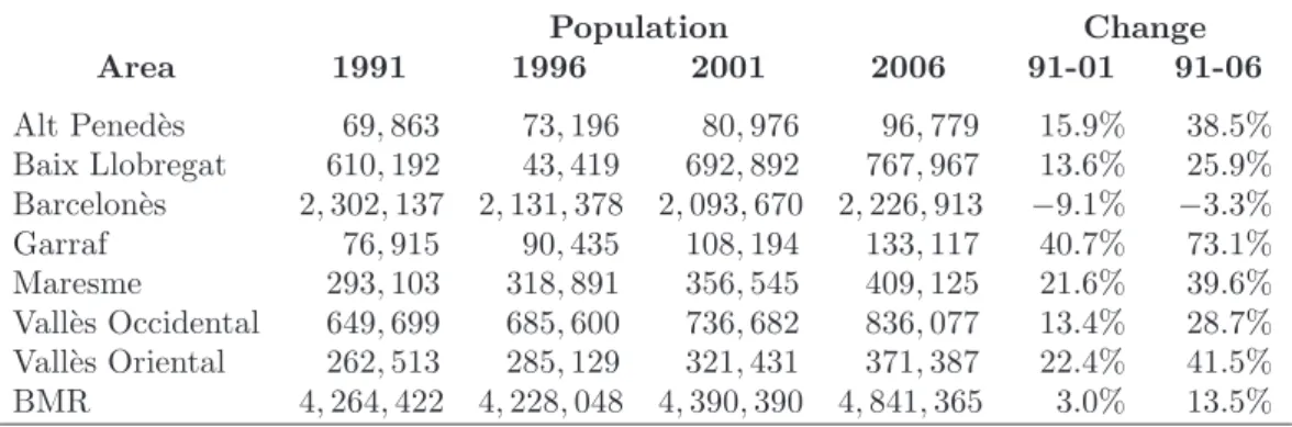
Table 1: BMR’s Population Growth and Change by Comarca
Population Change Area 1991 1996 2001 2006 91-01 91-06 Alt Pened`es 69,863 73,196 80,976 96,779 15.9% 38.5% Baix Llobregat 610,192 43,419 692,892 767,967 13.6% 25.9% Barcelon`es 2,302,137 2,131,378 2,093,670 2,226,913 −9.1% −3.3% Garraf 76,915 90,435 108,194 133,117 40.7% 73.1% Maresme 293,103 318,891 356,545 409,125 21.6% 39.6% Vall`es Occidental 649,699 685,600 736,682 836,077 13.4% 28.7% Vall`es Oriental 262,513 285,129 321,431 371,387 22.4% 41.5% BMR 4,264,422 4,228,048 4,390,390 4,841,365 3.0% 13.5%
With more than 4,800,000 inhabitants in 2006, the region’s population grew in almost 577,000 people during the previous 15 years (Table 1). This population growth process clearly benefited the 6 outer comarques with Vall`es Occidental and Baix Llobregat with the biggest gains (more than 150,000
13
Mu˜niz et al. (2008) considered these 13 municipalities as the CBC. 14
Vilafranca del Pened`es in Alt Pened`es, Vilanova i la Geltr´u in Garraf, Matar´o in Maresme, Sabadell and Terrassa in Vall`es Occidental.
15
Martorell in Baix Llobregat, Granollers in Vall`es Oriental. 16
Mu˜niz et al. (2003) provide an excellent overview of the historical process of the BMR’s metropolitan growth and formation.
inhabitants). On the contrary, the core “comarca”, Barcelon´es, although concentrating half of the region’s inhabitants, lost population (75,000 in-habitants). From a temporal point of view, the “absolute” decentralization process afecting Barcelon´es during the first 10 years was stopped by an in-tensive international migratory wave from Latin American countries and the new EU members. As abovementioned, this process also benefited the outer comarques and, as a result, the region underwent an internal population distribution.
Although these comarca aggregate figures show the existence of location changes in the BMR, they tell us little about the dynamics internal to the comarca boundaries, about the spatial organization of households in the re-gion. Paying attention to these issues requires to take into account the BMR’s urban spatial structure.
3.3. BMR’s Urban Spatial Structure
From an employment point of view, the BMR has been defined as
polycen-tric by Mu˜niz et al. (2008). Using municipal data, they applied a threshold
methodology based on Giuliano and Small (1991) in which an employment center is a municipality with an employment density greater than the BMR’s average density and an amount of employment greater than 1 per cent of the
BMR’s total employment. Besides the CBD17
, the authors found 9 employ-ment subcenters in 2001.
Regards population, the region has been also characterized as polycentric by Garcia-L´opez (2010). Using census tract data, centers are identified ap-plying McMillen (2003) methodology in which a non-parametric estimation is used (locally weighted regression). The idea is to estimate a population density function that represents a monocentric spatial structure. Using it
as a benchmark18
, the groups of significant deviations from the monocentric configuration (real densities greater than estimated densities) that surpass a population cutt-off are the centers. Defining Barcelona municipality as the main population center, the author identified 23 and 7 population subcen-ters in 2005 when cutt-offs of 10,000 inhabitants and 1 per cent of BMR’s
17
In fact, Mu˜niz et al. (2008) only identified employment subcenters and the CBD is defined as Barcelona and 12 adjacent municipalities with a continuous built-up area.
18
McMillen (2001) propose to use locally weighted regression because of its flexibility, allowing us to obtain any kind of monocentric benchmark and not only the imposed negative exponential function used by McDonald and Prather (1994).
inhabitants (47,701) are used, respectively.
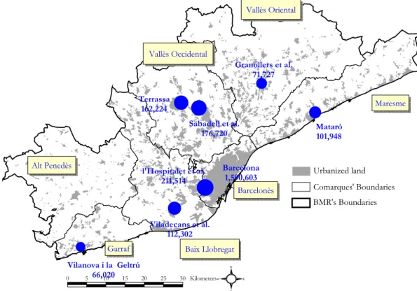
Figure 1: Urban Spatial Structure in the BMR: Centers
# # # # # # # Vilanova i la Geltrú 66,020 Mataró 101,948 Granollers et al. 71,727 Viladecans et al. 112,302 Terrassa 162,224 Sabadell et al. 176,720 l'Hospitalet et al. 211,514 Barcelona 1,590,603 Vallès Oriental Maresme Barcelonès Vallès Occidental Garraf Alt Penedès Baix Llobregat S N E W BMR's Boundaries Urbanized land Comarques' Boundaries 0 5 10 15 20 25 30 Kilometers
Although both type of subcenters are identified using different economic agents (employment and population), both groups are very similar. In this sense, 5 of the 7 largest population subcenters (Sabadell, Terrassa, Matar´o,
Granollers i Vilanova i la Geltr´u) (Figure 1) are also employment subcenters,
in fact the largest ones. Furthermore, they are also the abovementioned Christallerian towns with over a thousand years of history. Finally, because population data is available at a census tract level, the other 2 population
subcenters (l’Hospitalet i Viladecans) are located inside the Mu˜niz et al.
(2008)’s CBD and concentrate a large amount of employment. As a result, we use the 7 largest population subcenters to define the BMR’s urban spatial structure19
and analyze the spatial model in location and land consumption 19
patterns followed by population in the BMR.
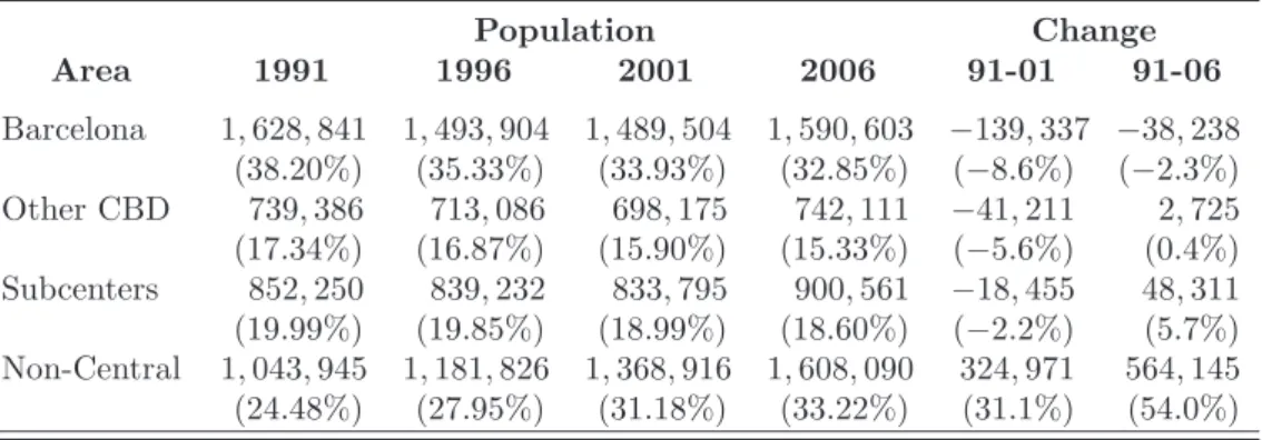
Taking into account this spatial structure, the location and land con-sumption trends of population in the BMR are shown in Tables 2 and 3. In this sense, Table 2 shows the number of inhabitants in each spatial area, its relative weight in the region and its absolute and relative variation in the first 10 years of the study, 1991-2001, as well as in the whole period ana-lyzed, 1991-2006. The figures show a suburbanization process characterized by the loss of population and relative importance of the CBD. Disaggregat-ing this spatial area between Barcelona municipality and the other 12 CBD municipalities20
we can see that the process is more intense in Barcelona municipality than in the rest of the CBD (8.6 vs 5.6 per cent of population decrease in 1991-2001). As was aforementioned, the arrival of migrants atten-uated this process, adding more than 100,000 and almost 44,000 inhabitants to Barcelona and the other CBD places, respectively.
Table 2: BMR’s Population Growth and Change by Area
Population Change Area 1991 1996 2001 2006 91-01 91-06 Barcelona 1,628,841 1,493,904 1,489,504 1,590,603 −139,337 −38,238 (38.20%) (35.33%) (33.93%) (32.85%) (−8.6%) (−2.3%) Other CBD 739,386 713,086 698,175 742,111 −41,211 2,725 (17.34%) (16.87%) (15.90%) (15.33%) (−5.6%) (0.4%) Subcenters 852,250 839,232 833,795 900,561 −18,455 48,311 (19.99%) (19.85%) (18.99%) (18.60%) (−2.2%) (5.7%) Non-Central 1,043,945 1,181,826 1,368,916 1,608,090 324,971 564,145 (24.48%) (27.95%) (31.18%) (33.22%) (31.1%) (54.0%)
The suburbanization process also afected the subcenters during the first 10 years in absolute and relative terms. In this sense, with a loss of more than 18,000 inhabitants (absolute suburbanization), their relative importance decreased from 20 to 19 per cent (relative suburbanization). Furthermore, although the migratory wave also benefited them adding almost 67,000 in-habitants between 2001 and 2006 and, as a result, increasing their population
and employment subcenters. 20
L’Hospitalet and Viladecans census tracts identified as subcenters are not included in the Other CBD Places computations.
in a 5.7 per cent in the whole period, their weight kept on decreasing and they came to concentrate only 18.6 per cent of population of the BMR.
Only the census tracts that make up the rest of the region, the Non-Central Places, are the ones that benefited from the suburbanization process afecting both the CBD and subcenters between 1991 and 2001, as well as from the growth of the region related to the migratory wave. With a popula-tion growth of 54 per cent, this area reached more than 1,600,000 inhabitants in 2006, increasing their relative importance from 24 to 33 per cent. Fur-thermore, only in 5 years, from 2001 to 2006, almost 240,000 individuals located in these places, 27,000 more than in the other areas together. As a result, it seems that these Non-Central Places were the main characters in the suburbanization process (1991-2001) and in the suburban growth process (2001-2006).
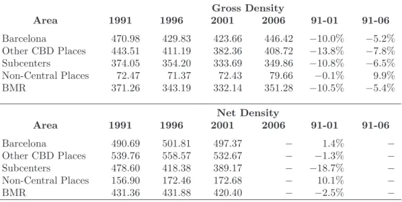
Table 3: BMR’s Average Density Growth and Change by Area
Gross Density Area 1991 1996 2001 2006 91-01 91-06 Barcelona 470.98 429.83 423.66 446.42 −10.0% −5.2% Other CBD Places 443.51 411.19 382.36 408.72 −13.8% −7.8% Subcenters 374.05 354.20 333.69 349.86 −10.8% −6.5% Non-Central Places 72.47 71.37 72.43 79.66 −0.1% 9.9% BMR 371.26 343.19 332.14 351.28 −10.5% −5.4% Net Density Area 1991 1996 2001 2006 91-01 91-06 Barcelona 490.69 501.81 497.37 − 1.4% − Other CBD Places 539.76 558.57 532.67 − −1.3% − Subcenters 478.60 418.38 389.17 − −18.7% − Non-Central Places 156.90 172.46 172.68 − 10.1% − BMR 431.36 431.88 420.40 − −2.5% −
Table 3 show the average density in each spatial area and its relative variation between 1991 and 2001 and between 1991 and 2006. Two types of population density are computed, the gross density, which measures the number of inhabitants per hectare of total land, and the net density, which measures the number of inhabitants per hectare of residential land. With the former density only population location is considered, with the latter we also consider the typology of the residential settlements and the consumption of
land, that is, location and land use jointly. In the gross density case, there is a trend to its reduction in all the spatial areas during the first 10 years. Due to the arrival of migrants, this trend was attenuated in all the areas, and even reversed in the Non-Central Places. In terms of population location and without taking into account the transport infrastructure, these figures show that the BMR’s spatial structure is becoming more dispersed, with lower density levels in its main centers (24-36 inhabitants) and slightly increasing densities in the periphery (9 inhabitants in Non-Central Places).
Paying attention not only to population location, but also to land con-sumption, allow us to detect dynamics slightly differents. In this sense,
al-though the average net density21
decreased 11 individuals per hectare in the whole region between 1991 and 2001, there was only one significant decrease in densities: the subcenters lost almost 90 inhabitants per hectare in av-erage. On the contrary, while Barcelona and Other CBD Places dynamics compensated each other, Non-Central Places density increased in almost 16 inhabitants per hectare of residential land. Taking into account that residen-tial land increased in 35.8 per cent, from 33,605 to 45,623 ha, between 1992 and 2002 (Garcia-L´opez, 2010) and that the most of this new residential land appeared in the Non-Central Places, the net density results of this spatial area show that people, although leaving the main centers and their higher densities, still prefer to live concentrated. As a result, the emergence of a more dispersed city is not clear when land consumption is considered.
Although Tables 2 and 3 results provide some insight into the BMR spatial structure characteristics and its most recent changes, they tell us little about the influence of the main centers on the location and/or land consumption of population outside them. Moreover, these results do not take into account the structuring role of transport infrastructure and, therefore, the possibility of an accessibility location model.
3.4. BMR’s Transport Infrastructure
The steep topography aforementioned, besides influencing its urbaniza-tion pattern, has also shaped the transport infrastructure network, which is mainly radial and connects the CBD with the subcenters and other main towns. More recently, transversal infrastructures have been built in order to
21
Computed using 1991, 1996 and 2001 population data and 1992, 1997 and 2002 resi-dential land data, respectively. Unfortunately, as was aforementioned, there is not a 2007 land use map available. As a result, 2006 net density was not computed.
reduce this radial pattern. This transport infrastructure is based on both a main road network and a railroad system that are very close to each other (Figures 2 and 3).
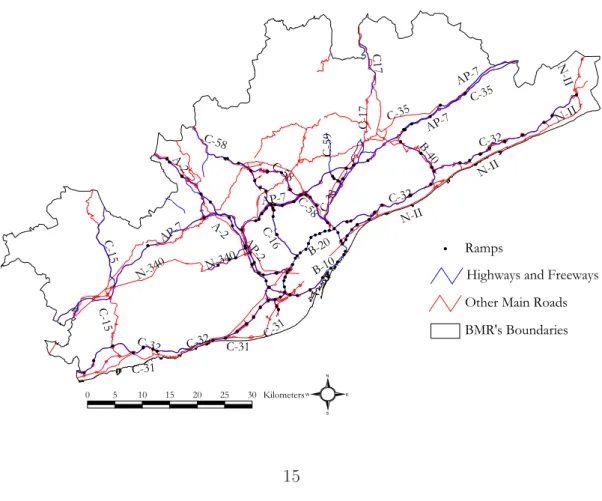
As for the main road network, it is based on several highways and freeways (A-2, AP-2, AP-7, C-16, C-17, C-32, C-33 and C-58) and other main roads (C-15, C-31, C-35, N-340, N-II, among others). The former are fast and high-capacity roads which their access are limited by ramps, and the latter are main roads that cross municipalities and have access from any point in the network. Although some highways-freeways were formerly other main roads with free access, most of them are new infrastructures, and, therefore, the capacity of the whole road network has increased. Nowadays, there are 516 km of highways-freeways, with 134 ramps located in 68 municipalities, and 670 km of other main roads. (Figure 2). In 2002 the main road network was about 16.25 per cent (11,047 ha) of the BMR’s urbanized area (Garcia-L´opez, 2010).
Figure 2: BMR’s Main Road Infrastructure
Ramps #
BMR's Boundaries Other Main Roads
Highways and Freeways # # # # # # # # # # # # # # # # # # # # # # # # # ## # # # # # # # # # # # # # # # # # # # # # # # # # # # # # # # # # # # # # # # # # # # # # # # # # # # # # # # # # # # # # # # # # # # # # # # # # # # # # # # # # # # # # # # # # # # # # # # # # # # # # # # # # # # N-340 AP-7 C-32 C-32 C-32 B-40 AP-7 C-33 AP-7 N-II C-15 C-58 AP-2 A-2 A-2 C-31 C-58 C-58 N-II C-35 C-32 C-17 C17 C-15 N-II N-340 C-16 C-31 C-31 N-II C-35 AP-7 C-59 B-20 B-10 S N E W 0 5 10 15 20 25 30 Kilometers
On the other hand, the railroad system is mainly a passenger-oriented
infrastructure with 1,172 km of railroad lines and 282 stations22
in 76 mu-nicipalities (Figure 3). It is based on an important subway (METRO), and some FGC and RENFE railroad lines. The former covers the whole munici-pality of Barcelona and partially the CBD and it is owned by a metropolitan public firm (Transports Metropolitans de Barcelona S.A.). The second are owned by a State public firm (Ferrocarrils de la Generalitat de Catalunya S.A.) and provide services to Barcelona, to some CBD’s municipalities and to some “comarques” nearest to Barcelona. And the latter are part of the National railroad system and communicate different parts of the BMR be-tween them and Barcelona (metropolitan services) and with the rest of the country (long-distance services).
Figure 3: BMR’s Railroad System and Stations
# # # # # # # # # # # # # # # # # # # # # # # # # # # # # # # # # # # # # # ## # # # # # # # # # # # # # # # # # # # # ## # # # # # # # # # # # # # # # # # # # # # # # # # ## # # # # # # # # # # # # # # # # # # # # # # # # # # # # # # # # # # # # # # # # # # # # # # # # # # # # # # # # # # # # # # # # # # # # # # # # # # # # # # # # METRO FGC METRO RENFE METRO METRO RENFE METRO METRO METRO FGC METRO RENFE RENFE METRO METRO # # # # # # # # # # # # # # # # # # # # # # # # # # # # # # # # # # # # # # # # # # # # # ## # # # # # # # # # # # # # # ## # # # # ## # # # # ## # # # # # # # # # #### # # # ## ## ## # # # # # # # # # # # # # # # # # # # # # # ## # ## # # # # # ## # # # # # # # # # # # # # # # ## # # # # # # # # # # # # # # # ### # # # # # # # # # # # # # # # # # # # # # # # # # # # # # # # # # # # # # # # # # # # # # # # # # # # # # # # # # # # # # # # # # # # # # # # # # # # # # # # # # # # # # # # # # # # # # # # # # # # # # # # # # # # # ## # # # # # # FGC FGC FGC FGC RENFE RENFE RENFE RENFE RENFE FGC FGC RENFE RENFE RENFE RENFE RENFE CBD's METRO SYSTEM BMR's Boundaries # Railroad Stations Railroad System S N E W 0 5 10 15 20 25 30 Kilometers 22
Barcelona concentrates 128 railroad stations, including subway stations, and there are 185 in the whole CBD. Most of them are subway stations.
4. Method
Following the NUE’s models, urban spatial structure should not be un-derstood merely as a phenomenon related to the amount of employment and population located in centers, for it is also the influence that these main cen-ters exercise on the location of the rest of the employment and population. This influence has been studied through the estimation of polycentric density functions in which density and distances to these centers are used as depen-dent and explanatory variables, respectively. The estimated coefficients to each center are called density gradients and measure whether density in-creases or reduces with distance to these centers. If it reduces for the CBD and subcenters, then centers influence is verified, as well as polycentricity. From a temporal point of view, decreasing (increasing) density gradients would show the reduction (increase) of the influence of these centers and, therefore, the emergence (reinforcement) of a more dispersed (polycentric) model.
As was mentioned in Section 2, NUE’s models also point out the role of transport infrastructure in determining the location and land consumption patterns (Steen, 1986; White, 1976; Sullivan, 1986). Including different dis-tances variables related to transport infrastructure we can study its influence on population location. As in the center case, infrastructure density gradi-ents that show a decreasing density pattern when we move away from this infrastructure would verify its influence and, therefore, the existence of the accessibility model. From a temporal point of view, increasing infrastructure gradients would show the reinforcement of this model.
In order to measure the influence of main centers and transport infras-tructure, we estimate the most common polycentric density function in which
the natural logarithm of the population density, 𝑙𝑛𝐷, is explained by the
dis-tance 𝑑𝐶𝐵𝐷 from the CBD and the inverted distance 𝑑
−1
𝑆𝑈 𝐵 from the nearest
subcenter (McDonald and Prather, 1994), and in which, testing different
specifications, we add different transport infrastructure distances 𝑑(∙).
As in Subsection 3.3, we use two types of population density. With the gross density (inhabitants per hectare of total land) we test main centers and infrastructure impact on population location, whereas with the net density (inhabitants per hectare of residential land) we estimate jointly their role on the location and land consumption of population.
4.1. Static Specifications
First of all, we estimate each density function following a static point of view, that is, for each year. The idea is to test, first, which of the following specifications is the best to explain the spatial distribution of population in the BMR. And, second, to determine which location model (polycentric, accessibility and/or dispersed model) prevails in the city.
Regarding specifications, in (1) we include a unique transport infrastruc-ture variable that summarize and assess the global role of “all transport infrastructure”. As aforementioned, using GIS software we merged main roads and railroads graphs and computed the distance to the nearest
trans-port infrastructure 𝑑𝐴𝐿𝐿. With this and the following variables we test the
existence of an accessibility model based on a parallel location close to this infrastructure. 𝑙𝑛𝐷=𝛼+𝛾𝐶𝐵𝐷𝑑𝐶𝐵𝐷 +𝛿𝑆𝑈 𝐵𝑑 −1 𝑆𝑈 𝐵 +𝜇𝐴𝐿𝐿𝑑𝐴𝐿𝐿 +𝜖 (1) To estimate the different influence of public transport based on the rail-road system and public and private transport that use the rail-road network,
specification (2) includes distance 𝑑𝑅𝐴𝐼𝐿 to the nearest railroad and distance
𝑑𝑅𝑂𝐴𝐷 to the nearest main road.
𝑙𝑛𝐷=𝛼+𝛾𝐶𝐵𝐷𝑑𝐶𝐵𝐷 +𝛿𝑆𝑈 𝐵𝑑 −1 𝑆𝑈 𝐵 +𝜇𝑅𝑂𝐴𝐷𝑑𝑅𝑂𝐴𝐷 +𝜇𝑅𝐴𝐼𝐿𝑑𝑅𝐴𝐼𝐿 +𝜖 (2) As aforementioned, the main road network is based on limited access roads (highways and freeways) and free access roads (other main roads). Using GIS software, we splitted main roads graph in these two main road
types and computed distance 𝑑𝐹 𝑅𝐸𝐸𝑊 to the nearest freeway-highway and
distance 𝑑𝑂𝑇 𝐻𝐸𝑅 to the nearest other main road. Specification (3) includes
these two variables instead of distance 𝑑𝑅𝑂𝐴𝐷 to the nearest main road.
𝑙𝑛𝐷=𝛼+𝛾𝐶𝐵𝐷𝑑𝐶𝐵𝐷 +𝛿𝑆𝑈 𝐵𝑑 −1 𝑆𝑈 𝐵 +𝜇𝐹 𝑅𝐸𝐸𝑊𝑑𝐹 𝑅𝐸𝐸𝑊 +𝜇𝑂𝑇 𝐻𝐸𝑅𝑑𝑂𝑇 𝐻𝐸𝑅 +𝜇𝑅𝐴𝐼𝐿𝑑𝑅𝐴𝐼𝐿+𝜖 (3)
By definition, access to highways and freeways are limited by ramps. These locations provide better accessibility than other parts of this
as an explanatory variable. Unlike the other transport infrastructure dis-tances , this variable allow us to take into account an accessibility model based on a concentric location pattern around these ramps. Specification (4)
still includes distance𝑑𝐹 𝑅𝐸𝐸𝑊 to the nearest freeway-highway as explanatory
variable because some of these freeways were formerly free access roads and, therefore, their previous influence might remain.
𝑙𝑛𝐷=𝛼+𝛾𝐶𝐵𝐷𝑑𝐶𝐵𝐷 +𝛿𝑆𝑈 𝐵𝑑 −1 𝑆𝑈 𝐵 +𝜇𝐹 𝑅𝐸𝐸𝑊𝑑𝐹 𝑅𝐸𝐸𝑊 +𝜇𝑅𝐴𝑀 𝑃𝑑𝑅𝐴𝑀 𝑃 +𝜇𝑂𝑇 𝐻𝐸𝑅𝑑𝑂𝑇 𝐻𝐸𝑅 +𝜇𝑅𝐴𝐼𝐿𝑑𝑅𝐴𝐼𝐿+𝜖 (4)
Finally, we include distance𝑑𝑆𝑇 𝐴𝑇 to the nearest railroad station in
speci-fication (5). Like in the freeway case, access to the railroad system is limited, in this case, to these stations. Taking into account this variable we test for the existence of an accessibility model based on a concentric location pattern around these stations. Unlike the previous specifications, we do not include
distance 𝑑𝑅𝐴𝐼𝐿 to the nearest railroad line because, obviously, access to this
infrastructure has been always limited to stations.
𝑙𝑛𝐷=𝛼+𝛾𝐶𝐵𝐷𝑑𝐶𝐵𝐷 +𝛿𝑆𝑈 𝐵𝑑 −1 𝑆𝑈 𝐵 +𝜇𝐹 𝑅𝐸𝐸𝑊𝑑𝐹 𝑅𝐸𝐸𝑊 +𝜇𝑅𝐴𝑀 𝑃𝑑𝑅𝐴𝑀 𝑃 +𝜇𝑂𝑇 𝐻𝐸𝑅𝑑𝑂𝑇 𝐻𝐸𝑅 +𝜇𝑆𝑇 𝐴𝑇𝑑𝑆𝑇 𝐴𝑇 +𝜖 (5)
In each estimation 𝛼 is the constant of the regression; 𝛾𝐶𝐵𝐷 and 𝛿𝑆𝑈 𝐵
are the CBD and subcenter density gradients, and the different 𝜇(∙) are the
density gradients associated with the several distances to the transport
in-frastructure (inin-frastructure gradients). 𝜖is the error term. Each specification
is estimated by ordinary least squares. In order to correct possible problems of heterocedasticity in the cross-section sample, standard errors and the co-variance matrix are calculated using White (1980)’s method.
The sign and significance of the estimated gradients provide us with the required information to discuss about the spatial configuration followed by BMR’s population. In this sense, a significant and negative value of the
CBD’s gradient (𝛾𝐶𝐵𝐷 <0) and a positive value of the nearest subcenter
gra-dient (𝛿𝑆𝑈 𝐵 >0) would show the existence of a polycentric structure in which
population density decreases as the inhabitants move further from the CBD and the nearest subcenter. The accessibility model, parallel and/or concen-tric, would be verified with a decreasing density pattern from the transport
infrastructure, that is, with a negative and significant infrastructure gradient
(𝜇(∙) < 0). Obviously, polycentricity and the accessibility model can
coex-ist. On the other hand, non-significant and/or positive gradients for CBD and infrastructure and a non-significant and/or negative subcenter gradient would show a dispersed spatial structure.
4.2. Dynamic Specification
The comparison of the static results for each year provides us with a first insight into the dynamics of the spatial structure. Increasing main cen-ters and/or infrastructure gradients (↑ 𝛾𝐶𝐵𝐷, ↑ 𝛿𝑆𝑈 𝐵, ↑ 𝜇(∙)) would indicate
the reinforcement of the polycentric and/or the accessibility model. On the contrary, decreasing gradients (↓ 𝛾𝐶𝐵𝐷, ↓ 𝛿𝑆𝑈 𝐵, ↓ 𝜇(∙)) would show that the
population spatial structure is evolving to a more dispersed location model. However, only comparing estimated gradients we do not know whether these changes are significant or not. In order to measure their significance, we estimate a density growth function using the same distances as explanatory variables:
Δ(𝑙𝑛𝐷) =𝛽𝛼+𝛽𝛾𝐶𝐵𝐷𝑑𝐶𝐵𝐷 +𝛽𝛿𝑆𝑈 𝐵𝑑 −1
𝑆𝑈 𝐵 +𝛽𝜇(∙)𝑑(∙) +𝜖 (6)
where Δ(𝑙𝑛𝐷) = 𝑙𝑛𝐷𝑡 −𝑙𝑛𝐷𝑡−1 measures population density changes, and
𝛽𝛾𝐶𝐵𝐷 =𝛾𝐶𝐵𝐷,𝑡−𝛾𝐶𝐵𝐷,𝑡−1,𝛽𝛿𝑆𝑈 𝐵 =𝛿𝑆𝑈 𝐵,𝑡−𝛿𝑆𝑈 𝐵,𝑡−1 and𝛽𝜇(∙) =𝜇(∙),𝑡−𝜇(∙),𝑡−1
test whether gradient changes are statistically significant (Small and Song, 1994; Garcia-L´opez, 2010). A significant and positive growth gradient for the
CBD (𝛽𝛾𝐶𝐵𝐷 >0), a significant and negative growth gradient for the case of
the nearest subcenter (𝛽𝛿𝑆𝑈 𝐵 < 0) and a significant and positive
infrastruc-ture growth gradient (𝛽𝜇(∙) >0) would show that population density grows
faster far away from these locations and, as a result, the suburbanization process is related to the emergence of the dispersed model. On the contrary,
a significant and negative infrastructure growth gradient (𝛽𝜇(∙) < 0) and/or
a significant and positive subcenter growth gradient (𝛽𝛿𝑆𝑈 𝐵 >0) would
indi-cate that the accessibility model and/or polycentricity are strengthened, even
when the suburbanization process is taking place in the CBD (𝛽𝛾𝐶𝐵𝐷 >0).
5. Results
5.1. Specifications
Tables 4 and 5 show the results obtained with each of the five specifica-tions estimated for 2006 using gross density and for 2001 using net density as
dependent variables. In both cases, their results explain the same story: As a whole, transport infrastructure matters and influences the location of
popu-lation in the BMR, Eq. (1) (𝜇𝐴𝐿𝐿 <0). However, a different impact is found
when the main road network and the railroad system are analyzed separately,
Eq. (2): Population seems to live far away from main roads (𝜇𝑅𝑂𝐴𝐷 > 0)
and close to the railroad system (𝜇𝑅𝐴𝐼𝐿 <0). Considering the heterogeneity
inside the main road network, the influence of the free access main roads is
detected (𝜇𝑂𝑇 𝐻𝐸𝑅 <0), whereas the previous positive all main road gradient
now is related to limited access main roads (𝜇𝐹 𝑅𝐸𝐸𝑊 > 0), Eq. (3). Only
when ramps are considered, the impact of freeways on the population spatial
structure is detected (𝜇𝑅𝐴𝑀 𝑃 < 0), Eq. (4). Finally, when distance to the
nearest station replace the whole railroad system variable, the influence of this infrastructure is again found (𝜇𝑆𝑇 𝐴𝑇 <0), Eq. (5).
Table 4: Gross Density Specifications
2006 (1) (2) (3) (4) (5) 𝛼 6.189∗∗∗ 6.330∗∗∗ 6.358∗∗∗ 6.385∗∗∗ 6.440∗∗∗ (99.94) (97.43) (92.45) (91.93) (92.67) 𝛾𝐶𝐵𝐷 −0.086∗∗∗ −0.086∗∗∗ −0.091∗∗∗ −0.090∗∗∗ −0.089∗∗∗ (−25.68) (−27.50) (−29.75) (−30.04) (−31.06) 𝛿𝑆𝑈 𝐵 0.273∗∗∗ 0.278∗∗∗ 0.217∗∗∗ 0.223∗∗∗ 0.210∗∗∗ (8.54) (8.34) (6.82) (6.97) (7.03) 𝜇𝐴𝐿𝐿 −0.046∗∗ − − − − (−2.04) 𝜇𝑅𝑂𝐴𝐷 − 0.177∗∗∗ − − − − (5.49) 𝜇𝐹 𝑅𝐸𝐸𝑊 − − 0.258∗∗∗ 0.298∗∗∗ 0.384∗∗∗ (6.91) (7.64) (9.12) 𝜇𝑅𝐴𝑀 𝑃 − − − −0.066∗∗∗ −0.053∗∗ (−2.94) (−2.50) 𝜇𝑂𝑇 𝐻𝐸𝑅 − − −0.056∗∗ −0.051∗ −0.042 (−1.93) (−1.76) (−1.47) 𝜇𝑅𝐴𝐼𝐿 − −0.208∗∗∗ −0.279∗∗∗ −0.237∗∗∗ − (−8.51) (−9.64) (−7.06) 𝜇𝑆𝑇 𝐴𝑇 − − − − −0.335∗∗∗ (−10.02) 𝑅2 0.3512 0.3770 0.3837 0.3867 0.4034 𝐴𝑘𝑎𝑖𝑘𝑒 3.3430 3.3027 3.2922 3.2876 3.2601
Paying attention to the explanatory capacity, 𝑅2
, and, above all, to the Akaike information criterion of each specification, the last one, Eq. (5), is the one that shows the highest and the lowest values, respectively. As a result, we use it to talk about the spatial model that households follow in their location and land consumption decisions in the BMR from a static point of view. Later, it is used as a benchmark to estimate the dynamic Equation (6) and analyze how the population spatial structure evolved between 1991-2001/6.
Table 5: Net Density Specifications
2001 (1) (2) (3) (4) (5) 𝛼 6.233∗∗∗ 6.327∗∗∗ 6.367∗∗∗ 6.386∗∗∗ 6.408∗∗∗ (160.41) (158.35) (147.17) (148.85) (148.49) 𝛾𝐶𝐵𝐷 −0.053∗∗∗ −0.053∗∗∗ −0.056∗∗∗ −0.056∗∗∗ −0.055∗∗∗ (−28.14) (−30.50) (−31.99) (−31.35) (−32.02) 𝛿𝑆𝑈 𝐵 0.140∗∗∗ 0.143∗∗∗ 0.107∗∗∗ 0.111∗∗∗ 0.109∗∗∗ (6.85) (6.78) (5.01) (5.22) (5.27) 𝜇𝐴𝐿𝐿 −0.040∗∗∗ − − − − (−2.91) 𝜇𝑅𝑂𝐴𝐷 − 0.099∗∗∗ − − − − (5.20) 𝜇𝐹 𝑅𝐸𝐸𝑊 − − 0.130∗∗∗ 0.158∗∗∗ 0.181∗∗∗ (5.50) (6.38) (6.97) 𝜇𝑅𝐴𝑀 𝑃 − − − −0.046∗∗∗ −0.046∗∗∗ (−3.58) (−3.78) 𝜇𝑂𝑇 𝐻𝐸𝑅 − − −0.048∗∗∗ −0.045∗∗ −0.045∗∗ (−2.60) (−2.43) (−2.44) 𝜇𝑅𝐴𝐼𝐿 − −0.132∗∗∗ −0.154∗∗∗ −0.125∗∗∗ − (−9.68) (−8.31) (−5.70) 𝜇𝑆𝑇 𝐴𝑇 − − − − −0.142∗∗∗ (−6.63) 𝑅2 0.3068 0.3313 0.3345 0.3380 0.3413 𝐴𝑘𝑎𝑖𝑘𝑒 2.5549 2.5193 2.5148 2.5098 2.5048 5.2. Static Results
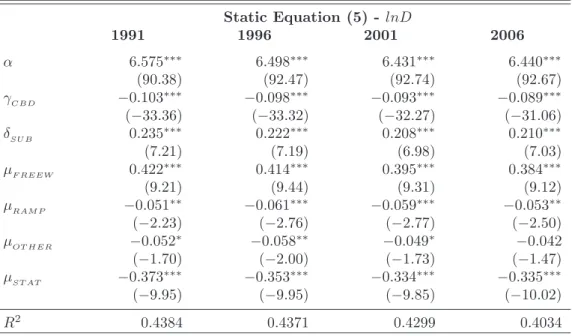
The static results (Tables 6 and 7) obtained with the selected specifica-tion, Eq. (5), show that the spatial distribution of population in the BMR
follows both a polycentric and an accessibility model. Furthermore, the ac-cessibility model is related to a concentric pattern around ramps and rail-road stations and to a parallel pattern close to other main rail-roads. In this
sense, the significant and negative CBD gradient (𝛾𝐶𝐵𝐷 <0) and the
signifi-cant and positive subcenter gradient (𝛿𝑆𝑈 𝐵 >0) confirm econometrically the
polycentric model, while the significant and negative infrastructure gradi-ents (𝜇(∙) <0) are consistent with the accessibility model. Only the positive
gradients related to the freeways-highways (𝜇𝐹 𝑅𝐸𝐸𝑊 > 0) show an
increas-ing density pattern from this infrastructure and, therefore, its inability to structure population location and land consumption decisions.
Table 6: Gross Density Location Patterns
Static Equation (5) - 𝑙𝑛𝐷 1991 1996 2001 2006 𝛼 6.575∗∗∗ 6.498∗∗∗ 6.431∗∗∗ 6.440∗∗∗ (90.38) (92.47) (92.74) (92.67) 𝛾𝐶𝐵𝐷 −0.103∗∗∗ −0.098∗∗∗ −0.093∗∗∗ −0.089∗∗∗ (−33.36) (−33.32) (−32.27) (−31.06) 𝛿𝑆𝑈 𝐵 0.235∗∗∗ 0.222∗∗∗ 0.208∗∗∗ 0.210∗∗∗ (7.21) (7.19) (6.98) (7.03) 𝜇𝐹 𝑅𝐸𝐸𝑊 0.422∗∗∗ 0.414∗∗∗ 0.395∗∗∗ 0.384∗∗∗ (9.21) (9.44) (9.31) (9.12) 𝜇𝑅𝐴𝑀 𝑃 −0.051∗∗ −0.061∗∗∗ −0.059∗∗∗ −0.053∗∗ (−2.23) (−2.76) (−2.77) (−2.50) 𝜇𝑂𝑇 𝐻𝐸𝑅 −0.052∗ −0.058∗∗ −0.049∗ −0.042 (−1.70) (−2.00) (−1.73) (−1.47) 𝜇𝑆𝑇 𝐴𝑇 −0.373∗∗∗ −0.353∗∗∗ −0.334∗∗∗ −0.335∗∗∗ (−9.95) (−9.95) (−9.85) (−10.02) 𝑅2 0.4384 0.4371 0.4299 0.4034
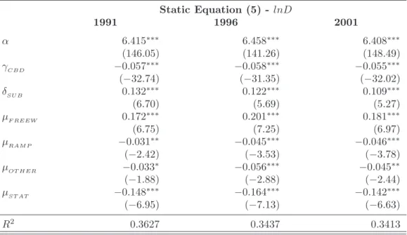
Regarding gross and net estimations, their results do not show significant differences in terms of gradient signs and significances. The only exception is distance to the nearest other main roads, which is not significant in 2006 when we only take into account population location patterns (growth density). Because we do not have data in residential land for this year to compute the net density, we do not know whether this also happened in the location and land consumption patterns. In terms of coefficient values, gross density results show steper gradients, that is, the fall of density in location terms is
higher than when location and land consumption patterns are considered. As a result, the density distribution is more homogeneous in net than in gross terms.
Table 7: Net Density Location and Land Consumption Patterns
Static Equation (5) - 𝑙𝑛𝐷 1991 1996 2001 𝛼 6.415∗∗∗ 6.458∗∗∗ 6.408∗∗∗ (146.05) (141.26) (148.49) 𝛾𝐶𝐵𝐷 −0.057∗∗∗ −0.058∗∗∗ −0.055∗∗∗ (−32.74) (−31.35) (−32.02) 𝛿𝑆𝑈 𝐵 0.132∗∗∗ 0.122∗∗∗ 0.109∗∗∗ (6.70) (5.69) (5.27) 𝜇𝐹 𝑅𝐸𝐸𝑊 0.172∗∗∗ 0.201∗∗∗ 0.181∗∗∗ (6.75) (7.25) (6.97) 𝜇𝑅𝐴𝑀 𝑃 −0.031∗∗ −0.045∗∗∗ −0.046∗∗∗ (−2.42) (−3.53) (−3.78) 𝜇𝑂𝑇 𝐻𝐸𝑅 −0.033∗ −0.056∗∗∗ −0.045∗∗ (−1.88) (−2.88) (−2.44) 𝜇𝑆𝑇 𝐴𝑇 −0.148∗∗∗ −0.164∗∗∗ −0.142∗∗∗ (−6.95) (−7.13) (−6.63) 𝑅2 0.3627 0.3437 0.3413 5.3. Dynamic Results
Tables 8 and 9 show the results of estimating Eq. (6) using the spec-ification finally selected, Eq. (5). In other to test whether the changes underwent during the whole period or, on the contrary, only took place in specific subperiods, we estimated the dynamic equation for the whole period
(1991-200123
and 1991-2006) and for each five-year period where data were available (1991-1996, 1996-2001, and 2001-2006).
In the gross density case (Table 8), the empirical results are consistent with the aforementioned suburbanization process affecting both the CBD and subcenters through the reduction of their influence on the location of
23
In order to compare gross and net results, we also estimated gross density changes for the first 10 years.
population (𝛽𝛾𝐶𝐵𝐷 = 0.014 > 0, 𝛽𝛾𝑆𝑈 𝐵 = −0.025 < 0). In the CBD case,
the process underwent during the whole period, whereas there was a slightly process of recentralization around the subcenters between 2001 and 2006 (𝛽𝛾𝑆𝑈 𝐵 = 0.001>0), although non-significant.
Table 8: Gross Density Location Changes
Dynamic Equation (6) -Δ(𝑙𝑛𝐷) 1991-1996 1996-2001 2001-2006 1991-2006 1991-2001 𝛽𝛼 −0.077∗∗∗ −0.067∗∗∗ 0.009 −0.136∗∗∗ −0.144∗∗∗ (−10.63) (−10.79) (0.80) (−7.98) (−12.83) 𝛽𝛾𝐶𝐵𝐷 0.005 ∗∗∗ 0.005∗∗∗ 0.004∗∗∗ 0.014∗∗∗ 0.010∗∗∗ (12.70) (18.69) (9.13) (18.30) (18.32) 𝛽𝛿𝑆𝑈 𝐵 −0.013 ∗∗∗ −0.014∗∗∗ 0.001 −0.025∗∗∗ −0.026∗∗∗ (−2.79) (−6.44) (0.49) (−3.55) (−4.68) 𝛽𝜇𝐹 𝑅𝐸𝐸𝑊 −0.007 −0.019∗∗∗ −0.011∗ −0.037∗∗∗ −0.026∗∗∗ (−1.35) (−4.55) (−1.67) (−3.35) (−3.36) 𝛽𝜇𝑅𝐴𝑀 𝑃 −0.010∗∗∗ 0.002 0.006∗∗ −0.002 −0.008∗∗ (−3.88) (0.80) (2.45) (−0.36) (−2.34) 𝛽𝜇𝑂𝑇 𝐻𝐸𝑅 −0.006 ∗∗ 0.009∗∗∗ 0.007 0.010 0.003 (−2.22) (3.68) (1.04) (1.10) (0.59) 𝛽𝜇𝑆𝑇 𝐴𝑇 0.020 ∗∗∗ 0.018∗∗∗ −0.001 0.038∗∗∗ 0.038∗∗∗ (3.95) (5.52) (−0.13) (4.18) (5.51) 𝑅2 0.1265 0.1135 0.0142 0.097 0.1612
As for the transport infrastructure, the more clear result is related to the freeways and highways: Although from an static point of view they were not places of high densities (with the exception of the ramps), be-tween 1991 and 2006 population density grew faster close to these main
roads (𝛽𝜇𝐹 𝑅𝐸𝐸𝑊 = −0.037 < 0). Only in the first five-year period the
changes were not significant. On the other hand, the access points of this infrastructure, the ramps, did not change significantly their influence on the location patterns. They began the period with an increasing influence (𝛽𝜇𝑅𝐴𝑀 𝑃 =−0.010<0). However, maybe because they got congestioned or
maybe because of the lack of available land around them, they finished the pe-riod with density growing faster far away from them (𝛽𝜇𝑅𝐴𝑀 𝑃 = 0.006 >0)
24
. 24
1991-Futhermore, there were not significant changes in the location patterns re-lated to the other main roads, although they lost influence during the last
ten years (𝛽𝜇𝑂𝑇 𝐻𝐸𝑅 > 0). Finally, the suburbanization process also affected
the railroad system through the lost of its influence during the whole period but, above all, in the first ten years (𝛽𝜇𝑆𝑇 𝐴𝑇 = 0.038>0).
As a whole, the gross empirical resuts are consistent with a polycentric model which is losing influence on the location pattern of population, but also with an accessibility model which is more based on a parallel location pattern close to freeways-highways and less on a concentric pattern around railroad stations.
Regarding net density results (Table 9), that is, taking into account lo-cation and land consumption patterns, the suburbanization process is also detected affecting both the CBD and subcenters between 1991 and 2001 (𝛽𝛾𝐶𝐵𝐷 = 0.002 > 0, 𝛽𝛾𝑆𝑈 𝐵 = −0.025 < 0). However, unlike the gross
den-sity case, this process underwent during the whole period in the subcenters case and only in the last five years in the CBD case.
From a transport infrastructure point of view, 1991-2001 density changes were only significant for the ramps, showing a significant increasing influ-ence (𝛽𝜇𝑅𝐴𝑀 𝑃 =−0.016 <0). Like the gross density results, this significant
increasing influence had its origin in the first five-year period (𝛽𝜇𝑅𝐴𝑀 𝑃 =
−0.015 < 0), whereas it was not significant between 1996 and 2001. In
the case of the freeway distance, its non-significant coefficient in 1991-2001 (𝛽𝜇𝐹 𝑅𝐸𝐸𝑊 = 0.007 > 0) is related to a positive and a negative significant
coefficient in 1991-1996 and 1996-2001, respectively. On the contrary, a sig-nificant increasing influence in the first five years and a sigsig-nificant decreas-ing influence in the last five years explain the non-significant coefficients
for the other main roads (𝛽𝜇𝑂𝑇 𝐻𝐸𝑅 = −0.012 < 0) and station distances
(𝛽𝜇𝑆𝑇 𝐴𝑇 = 0.006>0).
As a whole, the net empirical results are consistent with a spatial structure based on both polycentricity which is reducing its structuring role and an accessibility model which is reinforcing its concentric location pattern around ramps.
2001 changes and, as a result, the 1991-2006 changes were not significant. If these location changes continue in the future, the accessibility model related to this infrastructure will change from a concentric location pattern around ramps to a parallel location pattern close to the whole freeway-highway system.
Table 9: Net Density Location and Land Consumption Changes Dynamic Equation (6) -Δ(𝑙𝑛𝐷) 1991-1996 1996-2001 1991-2001 𝛽𝛼 0.051∗∗ −0.049∗∗∗ 0.002 (2.32) (−5.47) (0.11) 𝛽𝛾𝐶𝐵𝐷 −0.001 0.003∗∗∗ 0.002∗∗∗ (−1.01) (8.93) (3.02) 𝛽𝛿𝑆𝑈 𝐵 −0.012 ∗ −0.014∗∗∗ −0.025∗∗∗ (−1.68) (−4.58) (−3.26) 𝛽𝜇 𝐹 𝑅𝐸𝐸𝑊 0.027 ∗∗ −0.019∗∗∗ 0.007 (2.47) (−3.95) (0.59) 𝛽𝜇𝑅𝐴𝑀 𝑃 −0.015∗∗∗ −0.001 −0.016∗∗∗ (−2.76) (−0.47) (−2.76) 𝛽𝜇𝑂𝑇 𝐻𝐸𝑅 −0.022∗∗∗ 0.009∗∗∗ −0.012 (−3.12) (2.93) (−1.58) 𝛽𝜇𝑆𝑇 𝐴𝑇 −0.016 ∗ 0.023∗∗∗ 0.006 (−1.67) (6.03) (0.66) 𝑅2 0.0123 0.0386 0.0084 6. Conclusions
New Urban Economics recognizes that employment and population loca-tion is structured not only around main centers, but also around transport infrastructure. However, most theoretical and empirical studies still adopt a “main center point of view” considering only three alternatives types of urban spatial structure: Monocentricity, polycentricity and dispersion. By doing so, these works neglect the possibility of a more transport infrastructure-related urban form, the accessibility city, in which employment and population lo-cated in the non-central areas organize around the transport infrastructure in a parallel or concentric decreasing density pattern.
Departing from the traditional density functions, this paper has presented a thorough analysis of the population location and land consumption patterns and their evolution between 1991 and 2006 in the metropolitan Barcelona. Unlike previous studies, not only polycentricity and dispersion has been con-sidered as possible spatial models, but also the accessibility city. Further-more, different subtypes of accessibility location models has been studied.
that is a mix between polycentricity and the accessibility model. In this sense, not only main centers structure the location and land consumption patterns of population in the non-central areas, but also ramps, other main roads and railroad stations. Furthermore, the longitudinal results verify that the suburbanization process that underwent during the 15 years studied re-inforced this accessibility model, whereas main centers lost influence. As a result, if future spatial trends are similar to the ones detected in this study, the accessibility model will be the next preeminent spatial structure in the BMR.
References
Alonso, W., 1964. Location and Land Use. Toward a General Theory of Land Rent. Cambridge, MA: Harvard University Press.
Anas, A., Arnott, R., Small, K.A., 1998. Urban spatial structure. Journal of Economic Literature 36, 1426–1464.
Anderson, N., Bogart, W.T., 2001. The structure of sprawl - identifying and characterizing employment centers in polycentric metropolitan areas. American Journal of Economics and Sociology 60, 147–169.
Baum-Snow, N., 2007a. Did highways cause suburbanization? The Quarterly Journal of Economics 122, 775–805.
Baum-Snow, N., 2007b. Suburbanitzation and transportation in the mono-centric model. Journal of Urban Economics 62, 405–423.
Baumont, C., Ertur, C., Le Gallo, J., 2004. Spatial analysis of employment and population density. the case of the agglomeration of dijon 1999. Geo-graphical Analysis 36, 146–176.
Bogart, W.T., Ferry, W., 1999. Employment centres in greater cleveland: Evidence of evolution in a formerly monocentric city. Urban Studies 36, 2099–2110.
Bourne, L.S., 1989. Are new urban forms emerging? empirical test for canadian urban areas. Canadian Geographer 33, 312–328.
Cervero, R., Landis, J., 1997. Twenty years of the bay area rapid transit system: Land use and development impacts. Transport Research A 31, 309–333.
Cervero, R., Wu, K.L., 1997. Polycentrism, commuting, and residential lo-cation in the san francisco bay area. Environment and Planning A 29, 865–886.
Clusa, J., Roca, J., 1997. El canvi d’escala de la ciutat metropolitana de barcelona. Revista Econ`omica de Catalunya 33, 44–53.
Coffey, W.J., Shearmur, R.G., 2002. Agglomeration and dispersion of high-order service employment in the montreal metropolitan region. Urban Studies 39, 359–378.
Cox, W., Gordon, P., Redfearn, C.L., 2008. Highway penetration of central cities: Not a major cause of suburbanization. Econ Journal Watch 5, 32–45.
Forstall, R.L., Green, R.P., 1997. Defining job concentrations. the los angeles case. Urban Geography 18, 705–739.
Fujita, M., Ogawa, H., 1982. Multiple equilibria and structural transition of non-monocentric urban configurations. Regional Science and Urban Economics 12, 161–196.
Garcia-L´opez, M.A., 2010. Population suburbanization in barcelona,
1991-2005: Is its spatial structure changing? Journal of Housing Economics
Forthcoming.
Garcia-L´opez, M.A., Mu˜niz, I., 2011. Employment decentralisation:
Poly-centricity or scatteration? the case of barcelona. Urban Studies 48 Forth-coming.
Giuliano, G., Redfearn, C.L., 2007. Employment concentrations in los ange-les, 1980-2000. Environment and Planning A 39, 2935–2957.
Giuliano, G., Small, K.A., 1991. Subcenters in the los angeles region. Re-gional Science and Urban Economics 21, 163–182.
Gordon, P., Richardson, H.W., 1996. Beyond polycentricity: The dispersed metropolis, los angeles 1970-1990. Journal of the American Planning As-sociation 62, 289–295.
Gordon, P., Richardson, H.W., Wong, H.L., 1986. The distribution of pop-ulation and employment in a polycentric city. Environment and Planning A 18.
Gordon, P., Richardson, H.W., Yu, G., 1998. Metropolitan and
non-metropolitan employment trends in the us: Recent evidence and impli-cations. Urban Studies 35, 1037–1057.
Guillain, R., Le Gallo, J., Boietux-Orain, C., 2006. Changes in spatial and sectoral patterns of employment in ile-de-france, 1978-1997. Urban Studies 43, 2075–2098.
Lang, R.E., 2003. Edgeless Cities: Exploring the Elusive Metropolis. Wash-ington DC: Brookings Institution Press.
Lee, B., 2007. “edge” or “edgeless” cities? urban spatial structure in us metropolitan areas, 1980 to 2000. Journal of Regional Science 47.
Lucas, R.E.J., Rossi-Hansberg, E., 2002. On the internal structure of cities. Econometrica 70.
McDonald, J.F., 1987. The identification of urban employment subcenters. Journal of Urban Economics 21, 242–258.
McDonald, J.F., 1997. Fundamentals of Urban Economics. Upper Saddle River, NJ: Prentice Hall.
McDonald, J.F., Prather, P.J., 1994. Suburban employment centers: The case of chicago. Urban Studies 31, 201–218.
McMillen, D.P., 2001. Nonparametric employment subcenter identification. Journal of Urban Economics 50, 448–473.
McMillen, D.P., 2003. Identifying sub-centres using continguity matrices. Urban Studies 40, 57–69.
McMillen, D.P., McDonald, J.F., 1997. A nonparametric analysis of em-ployment density in a polycentric city. Journal of Regional Science 37, 591–612.
McMillen, D.P., McDonald, J.F., 1998. Suburban subcenters and employ-ment density in metropolitan chicago. Journal of Urban Economics 43, 157–180.
McMillen, D.P., Smith, S.C., 2003. The number of subcenters in large urban areas. Journal of Urban Economics 53, 321–338.
Mills, E.S., 1967. An aggregative model of resource allocation in a metropoli-tan area. American Economic Review 57, 197–210.
Mu˜niz, I., Galindo, A., Garcia-L´opez, M.A., 2003. Cubic spline population
density functions and satellite city deliniation: The case of barcelona. Ur-ban Studies 40, 1303–1322.
Mu˜niz, I., Garcia-L´opez, M., Galindo, A., 2008. The effect of employment
sub-centres on population density in barcelona. Urban Studies 45, 627–649. Muth, R.F., 1969. Cities and Housing: The Spatial Pattern of Urban
Resi-dential Land Use. Chicago, IL: University of Chicago Press.
Ogawa, H., Fujita, M., 1980. Equilibrium land use patterns in a nonmono-centric city. Journal of Regional Science 20, 455–475.
Ogawa, H., Fujita, M., 1989. Nonmonocentric urban configurations in a two-dimensional space. Environment and Planning A 21, 363–374.
Pfister, N., Freestone, R., Murphy, P., 2000. Polycentricity and dispersion? changes in center employment in metropolitan sydney. Urban Geography 41, 428–442.
Redfearn, C.L., 2007. The topography of metropolitan employment: Identi-fying centers of employment in a polycentric urban area. Journal of Urban Economics 61, 519–541.
Shearmur, R.G., Coffey, W.J., 2002. A tale of four cities: Intrametropolitan employment distribution in toronto, montreal, vancouver and ottawa-hull 1981-1996. Environment and Planning A 34, 575–598.