Joint Source-channel Coding Using Machine Learning Techniques

(1)

JOINT SOURCE-CHANNEL CODING USING MACHINE LEARNING

TECHNIQUES

An Undergraduate Research Scholars Thesis by

INIMFON I. AKPABIO

Submitted to the Undergraduate Research Scholars program at Texas A&M University

in partial fulfillment of the requirements for the designation as an

UNDERGRADUATE RESEARCH SCHOLAR

Approved by Research Advisor: Dr. Krishna Narayanan

May 2019

(2)

ABSTRACT

Joint Source-Channel Coding using Machine Learning Techniques

Inimfon I. Akpabio

Department of Electrical and Computer Engineering Texas A&M University

Research Advisor: Dr. Krishna Narayanan Department of Electrical and Computer Engineering

Texas A&M University

Most modern communication systems rely on separate source encoding and channel encoding schemes to transmit data. Despite the long-lasting success of separate schemes, joint source channel coding schemes have been proven to outperform separate schemes in applications such as video communications. The task of this research is to develop a joint source-channel coding scheme that mitigates some of the limitations of current separate coding schemes. My research will attempt to leverage recent advances in machine/deep learning techniques to develop resilient schemes that do not depend on explicit codes for compression and error correction but automatically learn end-to-end mapping schemes for source signals. The success of the

developed scheme will depend on its ability to correctly approximate an input vector under inconsistent channel conditions.

(4)

ACKNOWLEDGEMENTS

I would like to thank my advisor, Dr. Narayanan, and my TA, Ziwei Xuan for their guidance and support throughout the course of this research.

Thanks also go to my friends and colleagues and the department faculty and staff for making my time at Texas A&M University a great experience. I also want to extend my gratitude to my aunt, Dr. Imo Ebong for her continuous encouragement and support.

(5)

NOMENCLATURE

ML Machine-Learning DL Deep-Learning

JSCC Joint Source-Channel Coding DNN Deep Neural Network

FCNN Fully-Connected Neural Network SNR Signal to Noise Ratio

RNN Recurrent Neural Network LSTM Long Short-Term Memory

BRNN Bidirectional Recurrent Neural Network BLSTM Bidirectional Long Short-Term Memory MSE Mean Squared Error

BER Bit Error Rate BLER Block Error Rate

(6)

CHAPTER I

INTRODUCTION

Most modern communication systems perform two processes separately before

transmitting data over a channel: source coding and channel coding. Source coding maps source symbols (or an original signal) to informational symbols in order to eliminate redundancy from the source symbols and transmit information in the most efficient way possible. Channel coding adds redundancy to the coded signal to increase its integrity and allow for error detection and correction. Shannon's source-channel separation theorem [1] implies that we can achieve optimality in communication systems using separate source and channel coders given discrete memoryless channels and infinite block-length.

In reality, practical conditions preclude us from using large blocklengths. For example, modern engineering applications such as tactile internet require extremely low latency which ultimately prevent larger blocklength coding techniques [2]. Moreover, separation-based schemes cannot take advantage of improved channel conditions. Hence, once the source coding and channel coding rates have been set in place, the quality of reconstructions remains

unchanged given that the channel capacity remains above the target rate. Conversely, if the channel conditions deteriorate beyond some threshold, the performance will decrease severely. In communication theory, this is known as the cliff effect.

(7)

communication systems. It has gained appeal amongst communication researchers due to its potential applications in areas like audio communications, video communications, space exploration and satellite transmission. JSCC schemes are also desirable for their ability to overcome the “cliff effect”. In this research, we will attempt to develop JSCC schemes using deep neural networks that can still perform normally under varying channel conditions. To show that this is possible, the inputs will be constrained to 8 unique 7-bit vectors.

In recent years, the results of deep-learning (DL) research have become pervasive in different facets of technology and information sciences. DL techniques have found numerous applications in the field of communications which include quantization, compression,

localization, channel modelling and prediction, modulation recognition, etc. [4]. Unfortunately, deep-learning research has not been successfully applied to communications systems on a commercial scale. The reason for this stems from the fact that the schemes utilized in

communication technologies have to be optimally designed and perfected to guarantee reliable data transmission. Consequentially, any novel scheme or approach to data transmission is held to very high standards of performance. Nonetheless, deep-learning techniques have shown the potential to re-invent modern communications systems. The aim of this research is to investigate whether we can achieve better transmission error rates than separation-based schemes using deep-learning techniques.

Of particular interest amongst these techniques is self-supervised learning using an autoencoder [5]. Self-supervised implies that no label information is provided during learning instead the input signal is used as the target variable. The architecture of denoising autoencoders closely resembles that of an end-to-end communication system and can be used to find

(8)

Recurrent neural networks (RNN) paired with long short-term memory (LSTM) have also gained a lot of popularity in recent years. Due to their hidden states, RNN’s are able to retain deep contextual information. RNN’s have been successfully applied to sequential problems such as speech recognition.

In this thesis, we show that using a bidirectional long short term memory autoencoder architecture, we can achieve better error rates (bit error rate, block error rate and mean squared error) than the Hamming code. Additionally, we will also show that our developed models our able to take advantage of improved channel conditions and degrade amicably when the channel condition deteriorates.

The rest of the paper is divided into methods, results and a conclusion. The methods section offers an in-depth discussion of the techniques employed in this research. The results section contains the simulation results of the developed models including the comparison with the Hamming code.

(9)

CHAPTER II

METHODS

Deep neural networks

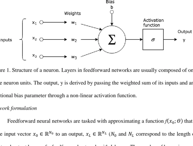
A deep-feedforward neural network forms the basis of most modern deep-learning models. The name neural network is loosely inspired by neuroscience, particularly studies on the human brain. Neural network models typically consist of one or more layers of neurons. The structure of such a neuron is shown in figure 1. Each neuron is responsible for generating output for its respective layer and works in parallel with other neurons. Hence, the outputs of a neural network layer are usually vector valued.

Figure 1. Structure of a neuron. Layers in feedforward networks are usually composed of one or more neuron units. The output, y is derived by passing the weighted sum of its inputs and an additional bias parameter through a non-linear activation function.

Network formulation

Feedforward neural networks are tasked with approximating a function f(𝑥0; 𝛳) that maps some input vector 𝑥0 ∈ ℝ𝑁0 to an output, 𝑥𝐿 ∈ ℝ𝑁𝐿 (𝑁0 and 𝑁𝐿 correspond to the length of the input and output layers of a feedforward network with 𝐿 layers. The number of layers in a network

(10)

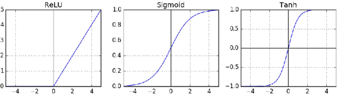
is usually referred to as the depth of the network.). Note that 𝑥0 and 𝑥𝐿 could represent classes in a feature space or categories in a classification problem. Feedforward networks, as they are called, propagate information computed from the input through a series of non-linear transformations to finally arrive at an output. These non-linear transformations are known as activation functions (𝜎) and are quintessential to the operation of neural networks. The added non-linearity allows deep feedforward networks to fully realize the benefits of stacking multiple layers on top of each other. Unlike purely linear models like linear regression, feedforward networks are able to describe more complex functions. Popularly used non linearities include rectified linear unit (ReLU) [6], tanh, sigmoid and softmax which are given below.

𝜎(𝑥) = max (0, 𝑥) (RELU) 𝜎(𝑥) = 𝑒𝑥−𝑒−𝑥 𝑒𝑥_+𝑒−𝑥 (Tanh) 𝜎(𝑥) = 1 1+𝑒−𝑥 (Sigmoid) 𝜎(𝑥_𝑖) = 𝑒𝑥𝑖 ∑ 𝑒𝑗 𝑥𝑗 (Softmax)

The ReLU is highly favored in deep-learning primarily because of the non saturation of its gradient which greatly improves the convergence of stochastic gradient descent compared to the sigmoid and tanh functions [7]. Others include: tanh, softmax, and sigmoid activation functions (see figure 2). The tanh activation function are heavily used in LSTMy units and are discussed in more detail in the recurrent neural network section. Softmax is often utilized in output layers of classification problem to output probability distributions for each output category.

(11)

Figure 2. ReLU, Sigmoid and Tanh activation functions.

The operation of a feedforward network can be thought of an iterative mapping of the outputs of the previous layer’s output by the current layer up till the final layer:

𝑧𝑖 = 𝑊𝑖𝑥𝑖−1+ 𝑏𝑖

𝑥𝑖 = 𝑓𝑖(𝑥𝑖−1; 𝛳𝑖) = 𝜎(𝑧𝑖), i = 1,…, L

The equations above apply to a standard fully-connected dense layer. Note that each mapping also depends on a set of parameters 𝛳. In this case, the parameters 𝑊_𝑖 and 𝑏_𝑖 constitute the parameter set for that layer. 𝑊_𝑖 is a trainable layer of weights and 𝑏_𝑖 is a trainable layer of biases.

Other layer types such as the Gaussian noise layer and the normalization layer exist in the following work. Although these layers are typically utilized for regularization purposes, we will use the Gaussian noise layer to simulate an additive white Gaussian noise channel and the normalization layer to satisfy the average power constraint. It is also worth noting that the mean and standard deviation used in normalization are calculated per batch.

𝑥_𝑖 = 𝑓_𝑖(𝑥𝑖−1) = 𝑥𝑖−1+ 𝒩(0, 𝑎𝐼𝑁𝑖−1) (Gaussian noise layer)

𝑥_𝑖 = 𝑓_𝑖(𝑥_𝑖−1) = (𝑥𝑖−1−𝑥̅𝑖−1) √(1 𝑚∑ (𝑥𝑖−1−𝑥̅𝑖−1) 2 𝑚 𝑘=1 )2+𝜖 (normalization layer)

(12)

Back-propagation

When a neural network is created, its parameters are initialized (initial values could be randomly set, fixed to zero, Gaussian distributed, etc.). Before such a network can be used to properly approximate some function, the network must adjust its parameters to the right values. This is achieved through training using a process known as back propagation. The purpose of back propagation is to adjust the parameters of the NN enough so that it approximates the desired function as closely as possible. During training, a set 𝑇 of input/output pairs are fed to the network and the closeness of the predicted output (𝑥_𝐿́ ) to the actual output (𝑥_𝐿) is quantified. The closeness of such an approximation is measured using what is known as a loss function.

𝐽(𝛳) = 1

||𝑇||∑𝑡∈𝑇𝑗(𝑥𝐿,𝑡, 𝑥𝐿,𝑡́ )

Many loss functions exist in machine-learning. For the purpose of this research, only 2 loss functions were used: mean squared error (MSE) and categorical cross-entropy. The MSE is simply the square of the Euclidean distance between the actual and predicted vector.

||𝑥_𝐿,𝑡− 𝑥_𝐿,𝑡́ ||2_(MSE)

− ∑𝑡∈𝑇𝑥𝐿,𝑡. log (𝑥𝐿,𝑡́ ) (Categorical Cross-entropy)

Categorical cross-entropy on the other hand is a cross-entropy generally following a softmax function. The softmax function which was mentioned earlier, outputs probability for each possible output class. Cross entropy loss measures the performance of a classifier that outputs a probability between 0 and 1. This loss increases as the output distribution diverges from the actual label distribution.

(13)

we update the set of parameters iteratively by taking steps in the opposite direction of the gradient of the loss function, which is calculated per mini-batch rather than using the entire dataset.

𝑊𝑖,𝑡 = 𝑊𝑖,𝑡−1 − 𝛾

𝜕𝐽 𝜕𝑊𝑖

The adjustments are usually regulated using a learning rate (𝛾). SGD has been proven to converge any convex loss function to a global minimum [8]. Another commonly used optimizer is the Adaptive moment estimation (ADAM) optimizer. Unlike SGD, ADAM computes an adaptive learning rate for each parameter. It achieves this by keeping track of a running average of exponentially decaying moments. In experiments involving deep feedforward NN’s with non-convex objective functions, ADAM often outperforms other optimizers [9].

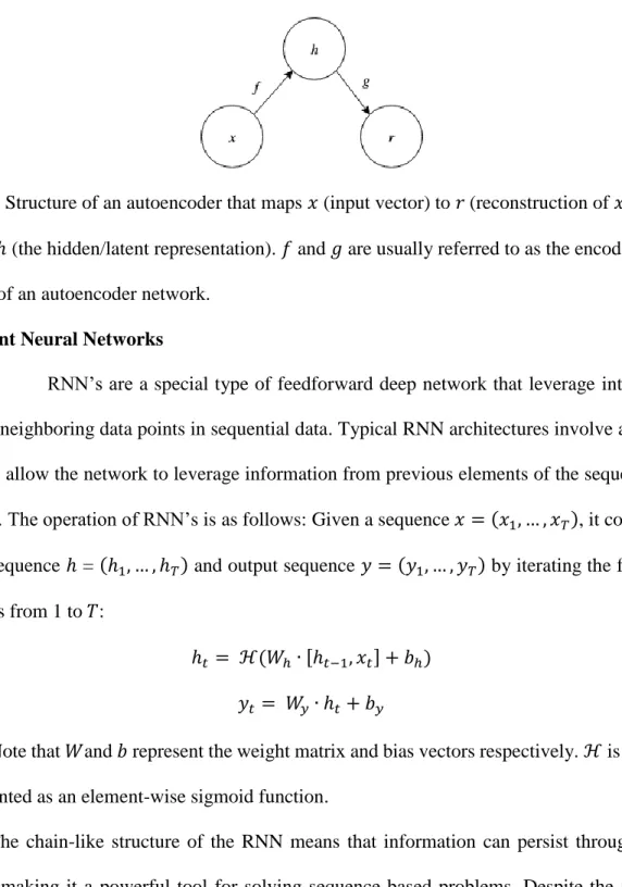
Autoencoders

Autoencoders are special types of feedforward networks that are applied to unsupervised learning tasks. These networks are tasked with reconstructing an output vector that is similar to its input. The architecture of an autoencoder shown in figure 3 is similar to that of an actual end-to-end communication system which makes it suitable for our experiments. In

minimizing the error between the input and the output the network learns a hidden layer

representation for mapping input signals. To avoid a trivial mapping of the inputs via an identity matrix, constraints are usually placed on the network. For instance, a noise layer could be added as a form of regularization. Such constraints usually allow the network to learn rich and

informative latent representations about the data. In our experiments, we leverage this as the noisy channel and learn an encoding scheme that maps a 7 bit vector to length-6 vector of real numbers.

(14)

Figure 3. Structure of an autoencoder that maps 𝑥 (input vector) to 𝑟 (reconstruction of 𝑥) through ℎ (the hidden/latent representation). 𝑓 and 𝑔 are usually referred to as the encoder and decoder of an autoencoder network.

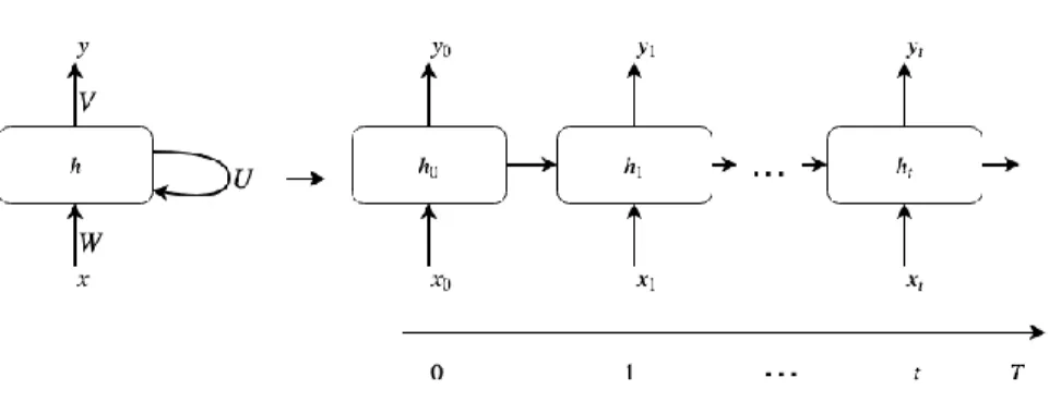
Recurrent Neural Networks

RNN’s are a special type of feedforward deep network that leverage interactions between neighboring data points in sequential data. Typical RNN architectures involve a delayed output to allow the network to leverage information from previous elements of the sequence (see figure 4). The operation of RNN’s is as follows: Given a sequence 𝑥 = (𝑥₁, … , 𝑥_𝑇), it computes a hidden sequence ℎ = (ℎ1, … , ℎ𝑇) and output sequence 𝑦 = (𝑦1, … , 𝑦𝑇) by iterating the following equations from 1 to 𝑇:

ℎ_𝑡 = ℋ(𝑊_ℎ∙ [ℎ_𝑡−1, 𝑥_𝑡] + 𝑏ℎ)

𝑦_𝑡 = 𝑊_𝑦∙ ℎ_𝑡+ 𝑏_𝑦

Note that 𝑊and 𝑏 represent the weight matrix and bias vectors respectively. ℋ is typically implemented as an element-wise sigmoid function.

The chain-like structure of the RNN means that information can persist throughout the network making it a powerful tool for solving sequence-based problems. Despite the ability to retain information, basic RNN’s lack the ability to retain long-term information. This is a direct

(15)

values, hence, resulting in little or no change to the network’s parameters. Fortunately, the introduction of LSTM in RNN models has helped to mitigate this problem.

Figure 4. Recurrent Neural Network.

Long Short-Term Memory

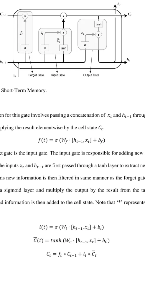
LSTM’s are basically a connection of recurrent blocks memory cell units. Each cell consists of 3 gates: input, forget and output gates that are effectively used to calculate its output, as in Figure 5. The power of the LSTM lies in its ability to propagate previous information through the cell state 𝐶𝑡 (i.e. the line running through the top of the network). Each cell unit can alter this information based on its interaction with either of the 3 gates. Gates usually consists of a multiplication operation to extract the features and a non-linear activation function that outputs a probability to filter how much information can pass through them (i.e. the sigmoid function outputs values between 0 and 1 which when multiplied by an input will select only a portion of the signal). The first gate is the forget gate. The forget gate selects how much information to retain from the cell state based on new input 𝑥𝑡 and ℎ𝑡−1 from the previous cell unit.

(16)

Figure 5. Long Short-Term Memory.

The computation for this gate involves passing a concatenation of 𝑥_𝑡 and ℎ_𝑡−1 through the sigmoid layer and multiplying the result elementwise by the cell state 𝐶_𝑡.

𝑓(𝑡) = 𝜎 (𝑊𝑓∙ [ℎ𝑡−1, 𝑥𝑡] + 𝑏𝑓)

The next gate is the input gate. The input gate is responsible for adding new information to the cell state. The inputs 𝑥_𝑡 and ℎ_𝑡−1 are first passed through a tanh layer to extract new information to be added. This new information is then filtered in same manner as the forget gate. We pass the input through a sigmoid layer and multiply the output by the result from the tanh layer. The resulting filtered information is then added to the cell state. Note that ‘*’ represents element-wise multiplication.

𝑖(𝑡) = 𝜎 (𝑊_𝑖∙ [ℎ_𝑡−1, 𝑥_𝑡] + 𝑏𝑖)

(17)

The output gate determines what information is output (ℎ𝑡) from each cell. It does this by applying a tanh layer to the cell state and filtering out the result with a sigmoid layer similarly to the input and forget gates.

ℎ_𝑡 = 𝑡𝑎𝑛ℎ (𝐶_𝑡) ∗ 𝜎 (𝑊_𝑜∙ [ℎ_𝑡−1, 𝑥_𝑡] + 𝑏_𝑜)

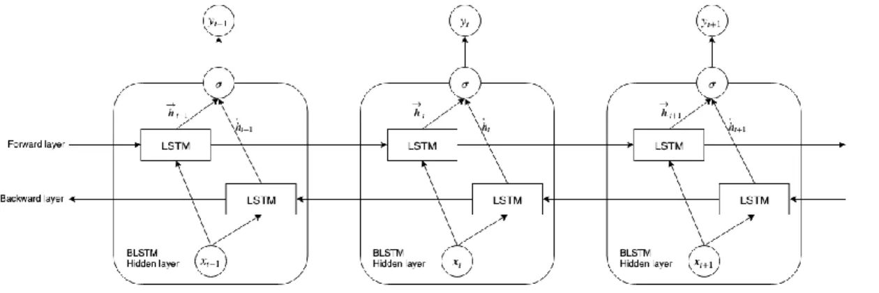
Although traditional LSTM’s have successfully been applied in areas such as speech recognition [10] and stock market analysis, they can only utilize sequential information in one direction (i.e. before or after). In order to fully overcome the aforementioned problem, we will introduce Bidirectional RNN’s (BRNN) which are able to utilize sequence information in both directions.

BRNN’s basically have 2 layers of RNN’s in parallel that handle training sequences in forward and backward directions (see figure 6). Both networks are connected to the output layer and this ensures that at every step in the sequence, the network can utilize past and future contextual information to minimize its loss. This also eliminates concerns over restrictions of the time-window since the network has enough contextual information at its disposal. A combination of BRNN’s and LSTM’s gives rise to the bidirectional LSTM (BLSTM). BLSTM’s leverage the bidirectional flow of information in RNN’s to retain past and future contextual information [11]. Alex and Jurgen in their experiments on Phoneme classification showed that bidirectional networks perform better than traditional unidirectional networks [12]. Bidirectional networks have also displayed great potential in various sequential problems [13], [14]. The next section describes the structure of our target model.

(18)

Figure 6. Bidirectional Recurrent Neural Network.

Implementation

A typical end-to-end communication system is made up of a transmitter, channel and receiver. The transmitter can send any of the allowed messages of blocklength 𝑘 with 𝑛 discrete uses of a channel. Hence the transmitter performs the mapping 𝑓 ∶ ℝ𝑘 ⟶ ℝ𝑛. Moreover, most communication systems place constraints on the transmitted signal (e.g. amplitude

constraint |𝑥_𝑖| ≤ 1 ∀𝑖). The transmitted signal is mapped using the transformation 𝑔 ∶ ℝ𝑛 _{⟶ ℝ}𝑘 to approximate the input signal.

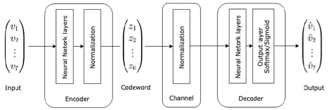
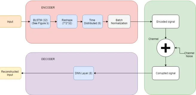
Figure 7 shows a structural representation of the target model architecture. The model will accept a 7-bit vector as input which will be mapped to a vector 𝑧 ∈ ℝ6. The encoded signal is then passed through a noisy channel which is simulated as an untrained layer of additive white Gaussian noise. The output of this channel is a corrupted signal which is then passed to the decoder that tries to recover/reconstruct the original signal. The 7-bit input vector is

(19)

Figure 7. Structural diagram of JSCC model architecture.

Despite using only 8 symbols, the addition of noise creates infinitely more input combinations to train the network with since the noise is modeled as a continuous random variable.

The models were trained using both MSE and categorical cross-entropy. Note that the model’s performance is measures using 3 major error metrics: bit error rate (BER), block error rate (BLER) and MSE. The bit error rate is simply a ratio of how many bits are incorrectly reconstructed/altered during transmission over all transmitted bits. Similarly, the block error rate is a ratio of how many vectors as a whole are wrongly reconstructed over all transmitted vectors. The mean squared error, on the other hand, is defined as the Euclidean distance between the reconstructed vector and the input vector and represents how far off the approximation is from the original input.

𝑀𝑆𝐸 = 1

7∑(𝑣𝑖 − 𝑣̂𝑖)

Multiple models were simulated and compared against the Hamming code in order to select the best model. The architectures for the deep-learning models were developed using Python2.7’s Keras libraries with Google’s TensorFlow as the backend. The results section focuses on the performances of the fully-connected neural network (FCNN) autoencoder and the

(20)

BLSTM autoencoder. To evaluate the reconstruction accuracy, the bit error rates and mean squared errors were measured and plotted against training epochs for different values of channel SNR.

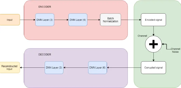
Fully-Connected Autoencoder

The network accepts the input and propagates it through a system of dense feedforward NN layers which will attempt to automatically learn an encoding scheme for the input (see figure 8). The encoding portion of the network consists of 2 hidden layers with 3 and 6 neurons

respectively connected to a normalization layer. The decision to use 3 neurons in the first hidden layer is incentivized by the number of information bits needed to encode 8 distinct symbols (source-coding). Additionally, it allows for a fair comparison to the Hamming code (see

Hamming code section). The second layer is fixed at 6 neurons to satisfy the desired number of discrete channel uses. The encoded signal is then normalized to satisfy the average signal power constraint according to 1

𝑛𝔼[𝑧 ∗ 𝑧] < 1 (where z is the encoded signal and 1 is the signal power constraint). This output of the encoder is a concise representation of the original input signal. The output of the encoder is then corrupted by the noisy channel simulated as a layer of additive white Gaussian noise before being passed on to the decoder. The decoder, on the other hand, decodes the channel codes by applying the learned decoding scheme and tries to find an approximate reconstruction of the source signal. Both the decoder and the encoder are trained simultaneously to maximize the conditional likelihood of a target vector given some input vector. Each dense layer uses ReLU activation function excluding the output layer which utilizes a softmax to output a probability distribution.

(21)

Figure 8. Functional Block diagram of FCNN autoencoder.

BLSTM Autoencoder

The BLSTM autoencoder model possesses a similar architecture to the FCNN

autoencoder albeit with different structural components as shown in figure 9. The encoder starts with a BLSTM stack/cell containing 7 hidden state units for each time step (see in figure 5). The dimensionality of the hidden units is set to 32 (see Recurrent Neural Network section for more details on the hidden state). Also recall from our earlier discussion on Bideirectional RNN’s that BLSTM contain 2 layers of LSTM working in parallel. Since these layers are not directly

connected to the final output, we will pass their hidden state values as output to the next layer. Hence the output dmiension of the BLSTM stack is (batch size, 7, 2*32). The next layer is an untrained reshape layer which squashes the 3-dimensional output of the BLSTM to a 1-dimensional vector of size (1, 2*7*32). The squashed vector is then passed on to a time distributed layer which maps it to a length-6 encoded vector as desired. The time distributed layer is a special type of layer in deep learning that is often used in conjunction with LSTM to

(22)

flatten the output from the preceding layer. Each time-step employs the same set of parameter values to perform its mapping. Similarly to the NDD autoencoder, we normalize the encoded vector and pass it through a channel to the decoder. The decoder in this case is simplistic and consists merely of an output layer with a softmax activation function.

Figure 9. Functional Block diagram of BLSTM autoencoder.

Hamming code

A shortened version of the (7, 4) hamming code is used as a benchmark for our

experiments. This modification involves fixing one of the information bits to zero. Hence this bit never changes and need not be transmitted resulting in a (6, 3) Hamming code.

(23)

The resulting codewords are first modulated using BPSK and decoded using 2 different methods: soft/block-wise decoding and hard/bit-wise decoding. For hard decoding we first the transmitted bits are converted to -1 or +1 based on the threshold (i.e. positive values are converted to +1 and negative values are converted to -1). Next we match the converted vector to the codeword with the minimum Hamming distance. For soft decoding the received vector is matched to the codeword with the minimum Euclidean distance.

(24)

CHAPTER III

RESULTS

Training Results

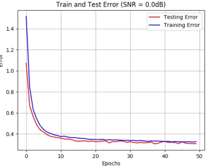
Figure 10 and figure 11 show the training and testing error results for FCNN autoencoder models trained on channels with 0.0 dB and 8.0 dB SNR respectively. The models were trained using 80,000 samples of data and tested on 20,000 samples using categorical cross-entropy loss. In our experiments, the ADAM optimizer displayed better convergence than other optimizers such as SGD and AdaGrad and was initialized with the following values: learning rate (0.001), beta1 (0.9), and beta2 (0.999). A lower batch size of 40 was found to yield better training results than using larger batch sizes like 256 or 512. We utilized checkpointing to retain the model state that yielded the best loss.

(25)

Figure 11. Training/Test Error for FCNN Autoencoder trained with 8.0 dB channel.

Figure 12 and figure 13 show the training and testing error results for BLSTM

autoencoder models trained on channels with 0.0 dB and 8.0 dB SNR respectively. Our BLSTM model converges faster than the FCNN and appears to reach a better global solution. This improved performance is due to the BLSTM’s ability to utilize contextual information in both the forward and backward direction as explained in the RNN section. The training parameters are similar to that of the FCNN.

The capacity of these models to converge to almost zero loss answers the major question of this research by showing that proving that deep-learning can indeed be used to develop Joint source-channel coding schemes. This is most likely due to the FCNN treating the noise layer as a regularization constraint. Consequentially, it is able to learn strong and robust hidden

(26)

(27)

Comparison with Hamming code

Figure 14 and 15 show the BER and BLER comparisons with the Hamming code. Surprisingly, the BLSTM autoencoder was able to match the Hamming code in terms of performance. This means that our BLSTM model was able to leverage its non-linearity to successfully learn a robust, Joint-coding scheme unlike the Hamming code which uses a linear transformation. It is worth noting that the Hamming code is not the fairest comparison since it is technically just a channel coding algorithm.

(28)

Figure 15. Block Error Rate comparison with hard and soft decision Hamming code.

Figure 16 shows the result of the MSE comparisons. To simulate the models against mean squared error loss, the output was modified to have the same dimension as the input. The results show that our models are still able to match the Hamming code in performance when trained with MSE loss for lower SNR values and levels off for higher values. Unlike the FCNN, the BLSTM’s ability to use bidirectional contextual information precludes it from getting stuck at a local minimum. Further improvements could possibly be realized by using regularization techniques such increase sparsity so as to obtain a stronger hidden representation of the inputs.

(29)

(30)

CHAPTER IV

CONCLUSION

The results show that it is possible for deep learning architectures to perform as well as separate schemes without the need for expressly specified codes. We were also able to show that the BLSTM autoencoder is robust and performs better than the Hamming code for varying channel SNR values. One of the shortcomings of this research is that the source blocklength is small compared to typical transmissions such as images. For such models to be deployed in practical applications, it might be necessary to develop different architectures to deal with different input types like text, images, etc. The models also need to be scalable and will require more rigorous training to properly operate in real-time.

(31)

REFERENCES

[1] Claude E Shannon and Warren Weaver, "The mathematical theory of communication", University of Illinois press, 1998.

[2] E. Bourtsoulatze, D. Burth Kurka, and D. Gunduz, “Deep joint source-channel coding for wireless image transmission,” ArXiv e-prints, Sep. 2018.

[3] Fan Zhai, Yiftach Eisenberg, and Aggelos K Katsaggelos, "Joint source-channel coding for video communications," Handbook of Image and Video Processing, 2005.

[4] M. Ibnkahla, “Applications of neural networks to digital communications–A survey,” Elsevier Signal Processing, vol. 80, no. 7, pp. 1185–1215, 2000.

[5] I. Goodfellow, Y. Bengio, and A. Courville, Deep learning. MIT Press, 2016.

[6] Zeiler, Matthew D., Marc'Aurelio Ranzato, Rajat Monga, Mark Z. Mao, Kevin Yang, Quoc V. Le, Patrick Nguyen, Andrew W. Senior, Vincent Vanhoucke, Jeffrey Dean and Geoffrey E. Hinton. “On rectified linear units for speech processing.” 2013 IEEE

International Conference on Acoustics, Speech and Signal Processing (2013): 3517-3521.

[7] A. Krizhevsky, I. Sutskever, and G. E. Hinton. Imagenet classification with deep convolutional neural networks. In Advances in Neural Information Processing Systems 25, pages 1106–1114, 2012

[8] Bottou, Léon (1998). "Online Algorithms and Stochastic Approximations".

OnlineLearning and Neural Networks. Cambridge University Press. ISBN 978-0-521-65263-6

[9] Kingma, Diederik P. and Ba, Jimmy. Adam: A Method for Stochastic Optimization. arXiv:1412.6980 [cs.LG], December 2014.

[9] Graves, Alex, Mohamed, Abdel-rahman, and Hinton, Geoffrey. Speech recognition with deep recurrent neural networks. In Acoustics, Speech and Signal Processing (ICASSP), 2013 IEEE International Conference on, pp. 6645–6649. IEEE, 2013.

(32)

[10] Nariman Farsad, Milind Rao, and Andrea Goldsmith, "Deep learning for joint sourcechannel coding of text", arXiv preprint arXiv:1802.06832v1, 2018.

[11] Graves, A., Jaitly, N., and Mohamed, A.-R. (2013). Hybrid speech recognition with deep bidirectional LSTM. In Automatic Speech Recognition and Understanding (ASRU), 2013 IEEE Workshop on, pages 273–278.

[12] Graves, A., Schmidhuber, J.: Framewise Phoneme Classification with Bidirectional LSTM and Other Neural Network Architectures. Neural Networks 18(5-6), 602– 610 (2005b)

[13] Gers, F.A., Schraudolph, N., & Schmidhuber, J.(2002). Learning precise timing with LSTM recurrent networks. Journal of Machine Learning Research, 3, 115–143.

[14] Baldi, P., Brunak, S., Frasconi, P., Pollastri, G., and Soda, G. (2001). Bidirectional dynamics for protein secondary structure prediction. Lecture Notes in Computer Science, 1828:80–104.