Raising the level of abstraction : simulation of large chip multiprocessors running multithreaded applications

(1)

Raising the Level of Abstraction:

Simulation of Large Chip

Multiprocessors Running

Multithreaded Applications

Alejandro Rico Carro

Advisors:

Alejandro Ram´ırez Bellido

Mateo Valero Cort´

es

Submitted to the Departament d’Arquitectura de Computadors

for the degree of

Doctor of Philosophy in Computer Architecture

at the

Universitat Polit`

ecnica de Catalunya

· BarcelonaTech

(2)

(3)

Acta de qualificació de tesi doctoral

Curs acadèmic: 2012/2013 Nom i cognoms

Alejandro Rico Carro Programa de doctorat

Arquitectura de Computadors

Unitat estructural responsable del programa

Departament d’Arquitectura de Computadors

Resolució del Tribunal

Reunit el Tribunal designat a l'efecte, el doctorand / la doctoranda exposa el tema de la seva tesi doctoral titulada

Raising the Level of Abstraction: Simulation of Large Chip Multiprocessors Running Multithreaded Applications

Acabada la lectura i després de donar resposta a les qüestions formulades pels membres titulars del tribunal, aquest atorga la qualificació:

NO APTE APROVAT NOTABLE EXCEL·LENT (Nom, cognoms i signatura)

President/a

(Nom, cognoms i signatura)

Secretari/ària

Vocal

______________________, _______ d'/de __________________ de _______________ El resultat de l’escrutini dels vots emesos pels membres titulars del tribunal, efectuat per l’Escola de Doctorat, a instància de la Comissió de Doctorat de la UPC, atorga la MENCIÓ CUM LAUDE:

SÍ NO

Presidenta de la Comissió de Doctorat

Secretària de la Comissió de Doctorat

(4)

(5)

Abstract

The number of transistors on an integrated circuit keeps doubling every two years. This increasing number of transistors is used to integrate more processing cores on the same chip. However, due to power density and ILP diminishing returns, the single-thread performance of such processing cores does not double every two years, but doubles every three years and a half.

Computer architecture research is mainly driven by simulation. In computer architecture simulators, the complexity of the simulated machine increases with the number of available transistors. The more transistors, the more cores, the more complex is the model. However, the performance of computer architecture simulators depends on the single-thread performance of the host machine and, as we mentioned before, this is not doubling every two years but every three years and a half. This increasing difference between the complexity of the simulated machine and simulation speed is what we call the simulation speed gap.

Because of the simulation speed gap, computer architecture simulators are increasingly slow. The simulation of a reference benchmark may take several weeks or even months. Researchers are concious of this problem and have been proposing techniques to reduce simulation time. These techniques include the use of reduced application input sets, sampled simulation and parallelization.

Another technique to reduce simulation time is raising the level of abstrac-tion of the simulated model. In this thesis we advocate for this approach. First, we decide to use trace-driven simulation because it does not require to provide functional simulation, and thus, allows to raise the level of abstraction beyond the instruction-stream representation.

However, trace-driven simulation has several limitations, the most impor-tant being the inability to reproduce the dynamic behavior of multithreaded applications. In this thesis we propose a simulation methodology that employs a trace-driven simulator together with a runtime sytem that allows the proper simulation of multithreaded simulations by reproducing the timing-dependent dynamic behavior at simulation time.

Having this methodology, we evaluate the use of multiple levels of abstraction to reduce simulation time, from a high-speed application-level simulation mode to a detailed instruction-level mode. We provide a comprehensive evaluation of the impact in accuracy and simulation speed of these abstraction levels and also show their applicability and usefulness depending on the target evaluations. We also compare these levels of abstraction with the existing ones in popular computer architecture simulators. Also, we validate the highest abstraction level against a real machine.

One of the interesting levels of abstraction for the simulation of multi-cores is the memory mode. This simulation mode is able to model the performance

(6)

abstraction, previous works have used filtered traces that do not include L1 hits, and allow to simulate only L2 misses for single-core simulations. However, sim-ulating multithreaded applications using filtered traces as in previous works has inherent inaccuracies. We propose a technique to reduce such inaccuracies and evaluate the speed-up, applicability, and usefulness of memory-level simulation. All in all, this thesis contributes to knowledge with techniques for the sim-ulation of chip multiprocessors with hundreds of cores using traces. It states and evaluates the trade-offs of using varying degress of abstraction in terms of accuracy and simulation speed.

(7)

Acknowledgements

First of all, I want to thank my advisor, Alex Ramirez, and co-advisor, Mateo Valero. They gave me support, guidance and freedom to make my own decisions through all these years. I have learnt a lot from them not only technically, but also in many other aspects in life. Alex has an impressive ability to turn the smallest idea into great contributions. I also want to thank him for putting up with my pessimism and criticism when I have not been able to see the promise and value of an idea. Mateo’s clarity and experience clearly improved the quality of the work and helped put it in a broader context.

I also want to thank my mentor, Pradip Bose, and collaborators, Jeff Derby and Bob Montoye, during my internship at IBM TJ Watson Research Center. I felt their trust from the first day. Pradip was always helpful and willing to teach me even the most obvious things. I also want to thank Roberto and Jose. I also learnt a lot from Roberto, and without their friendship my internship would have not been the same.

I thank my mentor, Chris Adeniyi-Jones, during my internship at ARM. He provided me with all the resources I needed and gave me freedom to carry out the work on my way. I also want to mention Gabor, Andreas, Roxana and James for their help.

I also want to thank the funding bodies that supported this work. This thesis has been supported by the European Social Fund and the Departa-ment d’Universitats, Recerca i Societat de la Informaci´o of the Generalitat de Catalunya under the FI scholarship no. FI-2006-01133; the Spanish Min-istry of Education under the FPU scholarship no. AP2005-4245; the FP6 SARC project (contract no. FP6-27648); the FP7 ENCORE project (contract no. FP7-248647); the FP7 Mont-Blanc project (contract no. ICT-FP7-288777); the Eu-ropean Network of Excellence HiPEAC; and the Comisi´on Interministerial de Ciencia y Tecnolog´ıa (contract nos. TIN2004-07739-C0201, TIN2007-60625 and TIN2012-34557).

I also want to mention that CellSim and TaskSim are the effort of many people. Main contributors to CellSim were Felipe, David, Toni and Augusto. Main contributors to TaskSim were Felipe, Augusto, Milan, Carlos and Victor. Vull agrair a Felipe, Miquel, Oriol i Xevi pels bons moments tots aquests anys i les tertúlies de sobretaula. Quiero agradecer especialmente a Felipe. Estuvo ah´ı desde el primer d´ıa y me ha dado su amistad y apoyo durante todo este tiempo. També vull agrair especialment a Miquel. És un gran amic, sempre està a punt per ajudar i va ser un gran recolzament durant els primers mesos a IBM.

I also want to mention the members of the group: Augusto, Milan, Carlos, Karthikeyan, Victor, Puzo, Rajo, Paul, Isaac, Thomas and Ugi; and other

(8)

col-makes work a happy activity everyday.

Tambi´en quiero dar las gracias a mis padres Alejandro y Emilia, y a mi hermano Abel. Desde siempre me han apoyado en todo lo que he querido hacer, me han dado los recursos y libertad para hacerlo, y me han aguantado cuando no he estado en mis mejores momentos. Les agradezco tambi´en que me regalaran mi primer ordenador pocos meses antes de empezar la universidad y liberarme as´ı de una vida aburrida y darme la oportunidad de trabajar con ordenadores, algo que estoy disfrutando cada d´ıa gracias a ellos.

Quiero dar las gracias a Luna por su apoyo y amor estos últimos años. Es un placer estar con una persona que lo da todo, está siempre ah´ı para levantar el ánimo y te recuerda cada d´ıa que es lo más importante en la vida.

(9)

3.3 Methodology . . . 47 3.3.1 Tracing . . . 48 3.3.2 Simulation Infrastructure . . . 49 3.3.3 Simulation Process . . . 49 3.4 Implementation . . . 50 3.4.1 Instrumentation . . . 50 3.4.2 Runtime Integration . . . 52 3.4.3 Simulation Example . . . 53 3.5 Experiments . . . 54 3.6 Coverage . . . 58 3.7 Summary . . . 59

4 Multiple Levels of Abstraction 61 4.1 State of the art . . . 62

4.2 Application Representation Abstraction . . . 63

4.3 Model Abstraction . . . 64 4.3.1 Burst Mode . . . 65 4.3.2 Inout Mode . . . 66 4.3.3 Mem Mode . . . 67 4.3.4 Instr Mode . . . 68 4.3.5 Summary . . . 69 4.4 Speed-Detail Trade-Off . . . 69 4.5 Evaluation . . . 73

4.5.1 Application Scalability using Burst . . . 73

4.5.2 Accelerator Architectures using Inout . . . 77

4.5.3 Memory System using Mem . . . 79

(11)

5 Trace Filtering of Multithreaded Applications 81

5.1 Problem . . . 82

5.2 State of the Art . . . 84

5.3 Methodology . . . 85

5.4 Implementation . . . 88

5.4.1 Sample implementation . . . 90

5.5 Evaluation . . . 91

5.5.1 Trace Size . . . 92

5.5.2 Trace Generation Time . . . 92

5.5.3 Simulation Accuracy . . . 94

5.5.4 Simulation Speedup . . . 96

5.6 Limitations . . . 96

5.7 Summary . . . 98

6 Modeling the Runtime System Timing 101 6.1 Problem . . . 101 6.2 Runtime Analysis . . . 103 6.3 Runtime Modeling . . . 105 6.4 Evaluation . . . 107 6.5 Discussion . . . 109 6.6 Summary . . . 110 7 Conclusions 111 7.1 Contributions and Publications . . . 112

7.2 Impact . . . 113

7.2.1 Our Related Work . . . 113

7.2.2 Other Works using Our Work . . . 114

7.2.3 Our Non-Related Work . . . 116

7.3 Future Work . . . 117

Glossary 122

(12)

(13)

List of Figures

1.1 Transistor count, die size, technology node and transistor density

for a set of microprocessors from 1971 to 2012. . . 2

1.2 Single Thread Performance . . . 5

1.3 Simulation speed gap. . . 6

1.4 Thesis timeline . . . 9

1.5 Thesis organization. . . 10

2.1 The Cell/B.E. microprocessor architecture [100]. . . 14

2.2 The CellSim simulator. . . 16

2.3 Producer-consumer module example using CycleSim. . . 19

2.4 Example of communication between Producer and Consumer mod-ules in CycleSim. . . 19

2.5 Examples of architectures modeled using TaskSim. . . 21

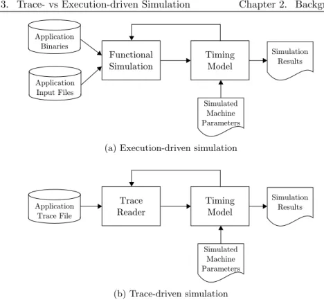
2.6 Flow chart of execution-driven and trace-driven simulation. . . . 23

2.7 Breakdown of papers per simulation type in main computer ar-chitecture conferences from 2008 to 2012 . . . 37

2.8 Breakdown of papers per maximum simulated number of cores in main architecture conferences from 2008 to 2012 . . . 38

2.9 Breakdown of papers per simulation tool in main computer ar-chitecture conferences from 2008 to 2012 . . . 39

2.10 Task-based implementation of the Fibonacci number recursive al-gorithm in (a) OpenMP 3.1, (b) Cilk and (c) Threading Building Blocks. . . 41

2.11 Cholesky decomposition of a blocked matrix using OmpSs. . . 42

3.1 Execution of an application with a mutual exclusion using two threads. . . 46

3.2 Simulation infrastructure scheme. . . 49

3.3 OmpSs application example and its corresponding traces for the TaskSim – NANOS++ simulation platform. . . 51

3.4 Implementation scheme. . . 52

3.5 Scheme of a multithreaded application simulation that generates 4 tasks and waits for their completion on two and four threads. . 54

3.6 Speed-up for different numbers of cores from 8 to 64 with respect to the execution with 8 cores. . . 55

3.7 Snapshot of the core activity visualization of a blocked-matrix multiplication a with 1 task-generation thread, and b with a hi-erarchical task-generation scheme . . . 56

(14)

core configurations. Speed-up with respect to the 16-core baseline. 57 4.1 Different application abstraction levels: (a) computation plus

MPI calls, (b) computation plus parops, (c) memory accesses, and (d) instructions. . . 63 4.2 Simulation error of the burst mode compared to the real

execu-tion on an eight-core AMD Opteron 6128 processor for multiple numbers of threads. . . 74 4.3 Comparison of real and simulated execution time for a 4096×4096

blocked-matrix Cholesky factorization using multiple block sizes. 76 4.4 Inout mode experiments on scratchpad-based architectures

us-ing an FFT 3D application: (a) execution on a real Cell/B.E., (b) simulation of a Cell/B.E. configuration, (c) simulation of a Cell/B.E. configuration using a 128 B memory interleaving gran-ularity, (d) simulation of a 256-core SARC architecture configu-ration using a 4 KB interleaving granularity, and (e) simulation of a 256-core SARC architecture configuration using a 128 B in-terleaving granularity. Light gray show computation periods and black shows periods waiting for data transfer completion. . . 78 4.5 Difference in number of misses between the mem and instr modes

for different simulated configurations using 4 and 32 cores, and different interleaving granularities. . . 79 5.1 Trace filtering: (a) example of a memory access trace, (b) how

trace filtering proceeds, and (c) the resulting filtered trace. . . . 82 5.2 Different multithread execution interleavings. On the left, the

invalidation occurs afterLOAD Dexecutes, soDhits. On the right, the invalidation occurs before Dso Dmisses in this case. If the trace is generated with the left execution, Dwill be filtered out, and if the scenario in the right is produced during simulation, D

will not be there to miss. . . 83 5.3 Different dynamic scheduling decisions. Iterations of a parallel

loop are scheduled in different ways. On the left, iterations 1 and 2 are assigned to Thread 0, and 3 and 4 to Thread 1. That makes iterations 2 and 4 to hit on their first memory access. On the right, 1 and 3 are assigned to Thread 0, and 2 and 4 to Thread 1, making all of them to miss on their first memory access. If the trace is generated using the left case and simulation leads to the case on the right, the first accesses in iterations 2 and 4 would not be present in the trace, and both misses could not be simulated. 83 5.4 Pathological case. The figure shows: (a) the pseudo-code of the

application; (b) the task dependence graph showing tasks in cir-cles and the arrows between them are read-after-write (solid) and write-after-read (dashed) dependencies; (c) the execution in a sin-gle thread used for trace generation with the order in which tasks are executed; and (d) the simulation of the application on four threads showing to which threads tasks are dynamically sched-uled and their execution order. . . 86

(15)

5.5 Pathological case execution time normalized to full trace with L2 cache latency of 20 cycles. A small L2 cache latency can be hid-den by the superscalar core microarchitecture. Longer latencies delay L1 misses that are correctly simulated with our methodol-ogy (reset) and using the full trace. The naive method does not simulate those L1 misses, as they were filtered out during trace

generation. . . 87

5.6 OpenMPfor loop construct. The figure shows: (a) a scheme of the execution flow of an OpenMPfor; (b) the original OpenMP C code and the intermediate C code generated by GCC, including the calls to thelibgompOpenMP runtime library. . . 89

5.7 Trace generation and simulation process. . . 90

5.8 Trace size reduction. . . 93

5.9 Trace generation speed-up. . . 93

5.10 Simulation accuracy. . . 95

5.11 Simulation accuracy average across benchmarks and frequencies. 96 5.12 Simulation speed-up. . . 97

5.13 Simulation speed-up average across benchmarks and frequencies. 98 6.1 Simulation example of a task-based application running on two threads. (a) The simulation alternates between the simulated threads and the runtime system operation, to simulate the ac-tions specified in the events included in the trace. The runtime system performs the creation of tasks, and assign tasks to idle threads (dashed line), such as Task 1 to Thread 1. (b) The simu-lation engine does not account the timing of the runtime system operations, and only simulates the timing of the sequential sec-tions in the trace. . . 102

6.2 Simplified pseudo-code of the main NANOS++ operations, and the actions on shared resources: task dependence graph and ready queue. Checks and updates of shared data are protected by locks or atomic operations depending on their granularity. . . 104

6.3 Runtime system operation variability. (a) Task creation cost dis-tribution of Cholesky factorization run on eight threads for two different throttling limits. (b) Breakdown of the lock contention time of Cholesky decomposition run on four, eight and sixteen threads for four different throttling limits. . . 105

6.4 Simulation example with host time only (left) and host time plus simulation of locks (right). . . 106

6.5 Normalized execution time real (a) and simulated (b,c,d) for a blocked-matrix multiplication using 64×64 blocks. . . 108

6.6 Task creation execution time of the H.264 decoder skeleton both in the real machine and using thehost simulation approach using multiple numbers of threads. . . 109

(16)

(17)

List of Tables

2.1 Main advantages and disadvantages of trace-driven simulation over execution-driven simulation . . . 28 2.2 Task-based programming models . . . 40 4.1 Summary of TaskSim simulation modes. This includes their

ap-plicability on computer architecture evaluations, and their fea-tures also comparing to state-of-the-art (SOA) simulators . . . . 69 4.2 Comparison of abstraction levels in existing simulators in terms

of simulation speed and modeling detail . . . 71 4.3 TaskSim main configuration parameters. The experiments in

Sec-tion 4.5 use the default values unless it is explicitly stated otherwise 73 4.4 List of benchmarks, including their label used in the charts and

a description of their configuration parameters. . . 74 4.5 Cholesky factorization of a 4096×4096 blocked-matrix using

dif-ferent block sizes. The table shows the number of tasks, the av-erage task execution time and the comparison of real execution and simulation for four and eight threads. . . 75 5.1 TaskSim simulation parameters. . . 91 5.2 OmpSs benchmarks. . . 92

(18)

(19)

Chapter 1

Introduction

1.1 Context and Motivation

1.1.1 Chip Multiprocessors

A microprocessor is an integrated circuit (chip) that incorporates the central processing unit (CPU) of a von Neumann-style computing system. The first microprocessors appeared in the early 1970s [176, 74]. Since then, the number of transistors on a chip has increased exponentially. This fact was observed by Gordon Moore in 1965, a claim that is popularly known as Moore’s law [124]. The rate at which the number of transistors on a chip increased was set to double every year in 1965. In 1975, Moore adjusted his observation to double every two years [123]. This observation has served as an industry driver. Com-panies’ roadmaps target Moore’s law transistor count growth rate, which sets targets for research and development divisions and results in the development and introduction of new technology nodes to achieve the required transistor density.

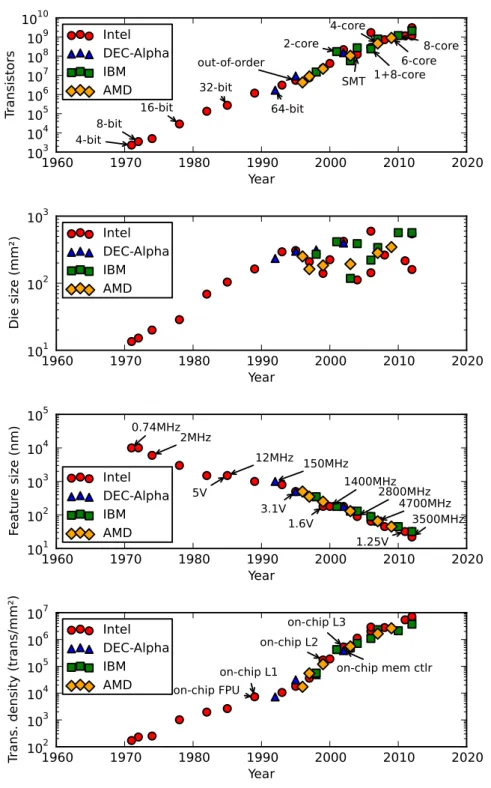
Figure 1.1 shows the transistor count per chip, die size, technology node and transistor density for a set of microprocessor from 1971 to 2012. Data actually confirms Moore’s law, and shows a 2x increase in transistor count per chip every two years. This increase was a combination of higher transistor density (+22%/year) and larger die size (+15%/year) until 1992. Since 1992, die size has not increased significantly. Server microprocessors have larger die sizes between 300 and 600 mm2_{, while desktop microprocessor die sizes are}

between 100 and 300 mm2_{. However, transistor density has increased 2x every}

two years (+40%/year) since 1992, thus keeping up with Moore’s law transistor count growth rate. This increase in transistor density growth rate was partially thanks to the inclusion of on-chip caches. Caches are more regular than other pipeline logic structures and thus have a higher transistor density.

The availability of more transistors allowed architects to integrate devices, that were so far out of the chip, on the chip (landmarks shown in transistor density chart in Figure 1.1). Examples are the inclusion of floating-point units, caches and memory controllers. Also, it allowed architects to build more com-plex architectures. First, the bit width of data and address paths was increased to improve performance and to be able to reference a larger address space. The first microprocessors had 4- and 8-bit data paths, with 16- and 32-bit

(20)

archi-1960

1970

1980

1990

2000

2010

2020

Year

10

3

10

4

10

5

10

6

10

7

10

8

10

9

10

Tra

nsi

sto

rs

4-bit

8-bit

16-bit

32-bit

64-bit

out-of-order

SMT

2-core

4-core

6-core

8-core

1+8-core

Intel

DEC-Alpha

IBM

AMD

1960

1970

1980

1990

2000

2010

2020

Year

10

1

10

2

10

3

Die

si

ze

(m

m²

)

Intel

DEC-Alpha

IBM

AMD

1960

1970

1980

1990

2000

2010

2020

Year

10

1

10

2

10

3

10

4

10

5

Fe

atu

re

siz

e (

nm

)

_0.74MHz2MHz

12MHz 150MHz

1400MHz

_2800MHz

4700MHz

3500MHz

5V

3.1V

1.6V

1.25V

Intel

DEC-Alpha

IBM

AMD

1960

1970

1980

1990

2000

2010

2020

Year

10

2

10

3

10

4

10

5

10

6

10

7

Tra

ns.

de

nsi

ty

(tr

an

s/m

m²

)

on-chip FPU

on-chip L1

on-chip L2

on-chip L3

on-chip mem ctlr

Intel

DEC-Alpha

IBM

AMD

Figure 1.1: Transistor count, die size, technology node and transistor density for a set of microprocessors from 1971 to 2012.

(21)

1.1. Context and Motivation Chapter 1. Introduction tectures appearing less than fifteen years later. The move from 32 to 64 bits took 18 years for personal computers. However, in the server market, where the system memory footprint is larger, there were 64-bit machines way earlier. An example is the DEC Alpha 21064 introduced in 1992.

Having smaller transistors also allowed to increase frequency, and thus in-crease performance. This inin-crease in frequency also came together with a reduc-tion in capacitance and voltage (landmarks shown in technology node chart in Figure 1.1). This scale down of voltage for smaller feature sizes was stated in a scaling theory by Robert Dennard et al. in 1974. This scaling theory is referred to as Dennard scaling. The result was that, having more and faster transis-tors together with a reduction in voltage and capacitance, new design chips provided more performance at the same power. This enabled the introduction of complex architectural techniques to improve performance, such as specula-tion, out-of-order execution and simultaneous multithreading (SMT). Also, the pipeline structures, such as branch prediction tables, reorder buffer and issue queues, were enlarged to exploit more instruction-level parallelism.

However, Dennard scaling stopped in the early 2000s. Since then, new tech-nology nodes provide more transistors, but voltage does not scale down any more. Voltage is over 1V in desktops, laptops and servers and just below 1V in embedded systems. The result is that power density increases and, as a side effect, frequency cannot be scaled up because affordable heat dissipation solutions cannot dissipate so much heat and the cooling solutions that would are too expensive. This limitation in power density is popularly known as the power wall. Moreover, at the same time, computer architects were experienc-ing diminishexperienc-ing returns in the latest improvements to exploit instruction-level parallelism [172, 143].

Under this scenario, microprocessor design shifted towards chip multipro-cessors or multi-cores. A multi-core is an integrated circuit including multiple processing cores, in contrast to the single processing core chips had so far. This design is more power efficient [38] and, as a result, more transistors can be used to increase performance by integrating more cores on the chip while preventing power density from skyrocketing.

The first academic paper proposing a multi-core design was presented in 1996 [132] and the first commercially-available multi-core was introduced in 2001. Since then, the trend is to include more cores per chip in every generation, which complicates their interconnection, the management of resources shared among cores and the programming of applications that shifted from focusing on instruction-level parallelism to targeting to exploit thread-level parallelism.

1.1.2 Chip Multiprocessor Simulation

Computer architecture research is mainly based on simulation. This is because the execution of a workload on a complex microprocessor can hardly be modeled analytically, and prototyping every design point is economically unviable.

In the 1980s and early 1990s, microprocessor simulators focused on the mod-eling of cache behaviour and the pipeline structures in the context of a single processing core per chip. Initially, pipeline models considered in-order execu-tion on a wider or narrower superscalar design. In time, the design complexity kept increasing with the introduction of increasingly complex techniques for out-of-order execution, speculation, branch prediction and simultaneous

(22)

multi-threading. On the other hand, the design space of the cache hierarchy included cache size, associativity, latency and writing policies for one or two cache levels. However, with the introduction of multi-cores, microprocessor simulation turned into the simulation of a parallel machine. The simulation of a parallel architecture is even more challenging than simulating a single core. Several execution streams stress not only coprivate components but also shared re-sources in the architecture. These shared components include shared caches, off-chip memory and the on-chip interconnection among cores. Modeling such sharing and resource contention is already challenging for multiprogrammed workloads. However, for multithreaded applications, it is also sensitive to the level of parallelism, inter-thread data sharing and thread synchronization of the particular application. To faithfully account for these effects, the simulation model requires the inclusion, among others, of cache coherence protocols, cache data placement policies, network arbitration and cache partitioning techniques. Many of the modeling challenges of multi-core simulation are not new, as they were already present when simulating shared-memory multiprocessor sys-tems with cache coherency across multiple chips. However, there are fundamen-tal differences of having such a parallel system on a single chip compared to multi-chip multiprocessors. Communication latencies are lower thanks to fast on-chip interconnection networks. And memory bandwidth is also lower because an increasing amount of processing cores have to share a limited amount of pins to access off-chip memory.

Due to these fundamental differences, researchers need to assess the applica-bility of techniques developed for shared-memory multiprocessors in the context of multi-cores. But, at the same time, multi-core designs also open new research opportunities that are unique for multi-cores. As a result, multi-core simulation becomes a fundamental tool for either revisiting existing ideas and explore new ones.

1.1.3 The Simulation Speed Gap

Computer architecture simulation is mainly a single-threaded problem because the fine-grain interaction of the components in the chip limits its parallelization. Most computer architecture simulators are thus sequential and, as a result, sim-ulation speed highly depends on the single-thread performance of the machine were the simulator is running.

While the complexity of microprocessors keeps increasing, single-thread per-formance is not increasing at the same pace. The efforts to develop or im-prove techniques to exploit instruction level parallelism have decreased due to diminishing returns and power density issues. This shifted the focus of com-puter architects to higher aggregated multi-core performance rather than higher single-thread performance.

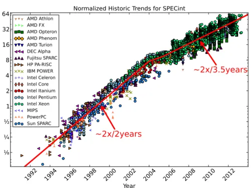
A popular benchmark suite to measure single-thread performance is SPEC (Standard Performance Evaluation Corporation) CPU. The SPEC CPU bench-mark suite is divided in two subsets: integer (CINT) and floating-point (CFP) benchmarks. We focus on the SPEC CINT benchmarks because computer sim-ulation code is mainly integer code. We have gathered the SPECint results for a set of microprocessors from 1991 to 2013 and adjusted them1 _{to the 2006}

(23)

1.1. Context and Motivation Chapter 1. Introduction

199

2

199

4

199

6

199

8

200

0 _Year

200

2

200

4

200

6

200

8

201

0

201

2 ⅛

¼

½

1

2

4

8

16

32

64 ~2x/2years

~2x/3.5years

Normalized Historic Trends for SPECint

AMD Athlon AMD FX AMD Opteron AMD Phenom AMD Turion DEC Alpha Fujitsu SPARC HP PA-RISC IBM POWER Intel Celeron Intel Core Intel Itanium Intel Pentium Intel Xeon MIPS PowerPC Sun SPARC

Figure 1.2: Single Thread Performance

standard to show the historical trends for single-thread integer performance. Figure 1.2 shows these results. Until 2004, integer performance doubles ap-proximately every two years. In 2004, multi-cores start becoming mainstream and, in some cases, the first approaches to multi-core design were to integrate simpler cores than the ones in the latest single-core microprocessors. For this reason, from 2004 to 2006, the chart shows some stagnation in performance improvement. Since 2006, single-thread performance improves again, but now it doubles approximately every 3.5 years.

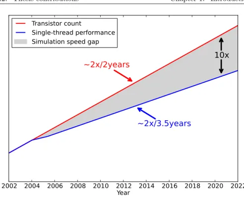
While single-thread performance improvement slows down, the complexity of multi-cores keeps increasing at the same pace thanks to the still-increasing amount of transistors per chip (see Figure 1.1). This translates into two facts. The complexity of the simulation model, which depends on the complexity of the simulated machine, keeps increasing at 2x every 2 years. But, the improvement on simulation speed, that depends on single-thread performance, is slowing down and improves at 2x every 3.5 years. This is what we call the simulation speed gap, and it is sketched in Figure 1.3. If the transistor count and single-thread performance trends hold for the next few years, there will be a 10x gap in around year 2020.

This increasing gap leads to increasingly longer simulation runs or to restrict the complexity of the model, for example, restrict the number of simulated cores. This fact is reflected in research works in top conferences where they use multi-core models with the same or less multi-cores than the ones in commercially-available products. While there are commercially-available multi-cores for conventional servers with 16 cores [46], and not so conventional with 64 [29], 79% of the

(24)

2002 2004 2006 2008 2010 2012 2014 2016 2018 2020 2022

Year

hola

~2x/2years

~2x/3.5years

10x

Transistor count

Single-thread performance

Simulation speed gap

Figure 1.3: Simulation speed gap.

research papers in major computer architecture conferences between 2009 and 2012 simulate at most 16 cores, and only 5% simulate more than 64 cores2_.

1.2 Thesis contributions

The simulation speed gap poses a challenge on computer architects to simulate large multi-core designs. To complete the simulation of large multi-cores in a reasonable time, we require higher simulation speeds. Researchers are concious of this problem, and they have proposed several techniques to reduce simulation time such as statistical simulation, sampling and parallel simulation.

The approach in this thesis is to raise the level of abstraction of the simula-tion model. This allows to increase simulasimula-tion speed at the expense of modeling accuracy in order to reduce simulation time. Some reputed researchers advocate for this approach [39, 180] and previous works have applied it in other scenarios such as cluster and network simulation [24, 120].

To implement high levels of abstraction, we advocate for the use of driven simulation. However, one of the most important limitations of trace-driven simulation is precisely its inability to reproduce the dynamic behavior of multithreaded applications, which are absolutely necessary for the evaluation of multi-core systems. This limitation is because the application behavior in multiple threads is statically captured in a trace and does not change for different simulated configurations as it would happen in a real machine.

To overcome this limitation, the first contribution in this thesis is:

(25)

1.2. Thesis contributions Chapter 1. Introduction • A simulation methodology for simulating multithreaded applications running on multi-cores using trace-driven simulation. In this simula-tion methodology, we combine the trace-driven simulasimula-tion of the timing-independent parts of the application, with the execution of timing-dependent operations at simulation time. This way, run-time decisions are made based on the simulated machine and are thus different for different config-urations as it would happen in the real machine. This work is supported by the following papers:

[150] A. Rico, A. Duran, F. Cabarcas, Y. Etsion, A. Ramirez, M. Valero. Trace-driven Simulation of Multithreaded Applications. In Proceed-ings of the IEEE International Symposium on Performance Analysis of Systems and Software, ISPASS ’11, pages 87–96, Apr. 2011. [151] A. Rico, A. Duran, A. Ramirez, M. Valero. Simulating

Dynamically-Scheduled Multithreaded Applications Using Traces. IEEE Micro. Submitted for publication.

Once we can reliably use trace-driven simulation for multithreaded applica-tions running on multi-cores, we use it to raise the level of abstraction of simu-lation. However, several questions arise when using higher levels of abstraction regarding what are the right levels of abstraction, their insight, accuracy and simulation speed.

The second contribution in this thesis is:

• Two fast high-level simulation modesalong with two lower-level ones. These simulation modes at different levels of abstraction are based on our definition of application abstraction levels and target application scala-bility, accelerator architectures, memory system and pipeline modeling, respectively. We evaluate the insight of these simulation modes, their ac-curacy and their simulation speed compared to the levels of abstraction used in popular computer architecture simulators. This contribution is supported by the following publication:

[148] A. Rico, F. Cabarcas, C. Villavieja, M. Pavlovic, A. Vega, Y. Etsion, A. Ramirez, M. Valero. On the Simulation of Large-Scale Architec-tures Using Multiple Application Abstraction Levels. ACM Trans. Archit. Code Optim., 8(4):36:1–36:20, 2012.

One of the abstraction levels in our definition targets multi-core memory simulation. This level of abstraction uses an abstract model for processing cores that focus mainly on memory accesses. To speed up memory simulation, previous works use filtered traces that include only L1 cache misses to avoid the cost of simulating L1 hits assuming that these do not imply additional delays in the simulated application. This technique, called trace stripping [138], has been successfully used in the past for single-thread scenarios. However, little work has been done to use it for multithreaded applications, in which inherent inaccuracies appear due to cache invalidations. A filtered hit may miss in a multithreaded scenario due to the invalidation of the accessed data from a write in another cache.

(26)

• A trace generation techniquebased on the structure of multithreaded applications that captures in the trace L1 hits that may potentially miss in a multithreaded application execution due to invalidations. With this technique, we cover potential invalidations due to different thread inter-leavings and different dynamic schedulings. Our evaluation shows that our technique consistently reduces the error of the state-of-the-art tech-nique at the expense of small losses in trace size reduction and simulation speed-up. This work is supported by the following publication:

[154] A. Rico, A. Ramirez, M. Valero. Trace Filtering of Multithreaded Applications for CMP Memory Simulation. In Proceedings of the IEEE International Symposium on Performance Analysis of Systems and Software, ISPASS ’13, pages 134–135, Apr. 2013.

One of the potential inaccuracies of our simulation methodology in our first contribution is that the execution of timing-dependent operations is not exposed to the simulator, and thus cannot be accurately accounted in the application timing modeling.

The fourth contribution in this thesis is:

• A fast high-level timing model for timing-dependent operations that are executed at simulation time using our simulation methodology. This timing model is based on the execution of these operations on the host machine to account for different algorithm complexities and run-time application states. Additionally, we also model their contention on accessing data structures shared by multiple threads on the simulated application.

1.3 Timeline

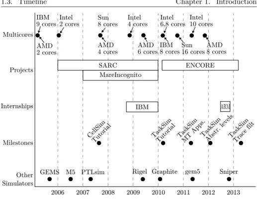
Figure 1.4 shows a timeline of relevant events related to the work in this thesis to put it in context. At the top of the figure, we show the releases of multi-core commercial products. The trend followed by the main manufacturers is to increase the number of cores per chip in every new generation of multi-cores. As explained in previous sections, this motivates our work to bridge the simulation-speed gap.

The work in this thesis has contributed to several projects. From January 2006 to December 2009, we contributed to the SARC project with the devel-opment of CellSim (see Section 2.1). CellSim served to carry out the work of several partners in the project, leading to multiple publications and PhD dissertations (see Section 7.2). CellSim was also the base for SARCSim: an ex-tension of CellSim including timing models from other SARC partners, such as models of extended vector accelerators and scalable inter-core communication mechanisms.

In the context of the MareIncognito project (from January 2007 to December 2009), CellSim was relevant in the research for the design of next-generation Cell/B.E. microprocessors (see Section 2.1.1). From March 2010 to February 2013 we contributed to the ENCORE project. The simulation methodologies proposed in this thesis were used in ENCORE for the evaluation of explicit management of coherent and non-coherent cache hierarchies. Also, the analysis

(27)

1.3. Timeline Chapter 1. Introduction 2006 2007 2008 2009 2010 2011 2012 2013 Multicores Projects Milestones Other Simulators CellSim Tutorial Internships IBM 9 cores SARC ENCORE MareIncognito IBM ARM TaskSim

Tutorial TaskSimMT Apps.TaskSimAbstr. levelsTaskSimTrace filt

gem5 Graphite Sniper Rigel Intel 2 cores AMD 2 cores AMD 4 cores Intel 4 cores AMD 6 cores Intel 6,8 cores IBM 8 cores Intel 10 cores AMD 8 cores Sun 8 cores Sun 16 cores GEMS M5 PTLsim

Figure 1.4: Thesis timeline

of the runtime system we carried out for the simulation of the runtime system timing (see Chapter 6) was used in ENCORE to understand the overheads of the several components in the runtime system.

The course of this thesis was interrupted by two industrial internships. The first one at the IBM TJ Watson Research Center (Yorktown Heights, NY, USA) for the development of a vector accelerator took place from October 2008 to December 2009. The second internship was at ARM Ltd. (Cambridge, UK) from August 2012 to November 2012 and focused on the evaluation of the ARM Cortex-A family of microprocessors for high performance computing.

Some milestones worth mentioning as outcomes of the work in this thesis are the following:

• CellSim Tutorial. We performed a full-day tutorial on our CellSim simulator (see Section 2.1) in the Parallel Architectures and Compilation Techniques (PACT) conference at Brasov, Romania, on September 2007. • TaskSim Tutorial. We performed a tutorial for the ENCORE project

partners on our TaskSim simulator (see Section 2.2) on March 2010. • Publication of ”Trace-Driven Simulation of Multithreaded

Ap-plications”. Publication in Proceedings of the International Sympo-sium on Performance Analysis of Systems and Software (ISPASS) 2011 at Austin, TX, USA, on April 2011.

• Publication of ”On the Simulation of Large-Scale Architectures Using Multiple Application Abstraction Levels”. Publication in the ACM Transactions on Architecture and Compiler Optimization (TACO), Vol. 8, No. 4, Article 36, January 2012.

(28)

• Publication of ”Trace Filtering of Multithreaded Applications for CMP Memory Simulation”. Publication in International Sympo-sium on Performance Analysis of Systems and Software (ISPASS) 2013 at Austin, TX, USA, on April 2013.

In the course of this thesis, other groups in the computer architecture com-munity working on simulation of multi-cores published their tools in related conferences and journals. Some of them shown at the bottom of Figure 1.4 are GEMS, M5, PTLsim, Rigel, Graphite, gem5 and Sniper. We cover these works in Section 2.5.

1.4 Thesis Organization

Figure 1.5 illustrates the organization of this document in the several chapters it is composed of.

1. Introduction

7. Conclusions

Publications Impact Future Work 3. Simulating Multithreaded

Applications Using Traces

4. Multiple Levels of Abstraction 5. Trace Filtering of Multithreaded Applications 6. Modeling the Runtime System Timing 2. Background CellSim TaskSim

Figure 1.5: Thesis organization.

After this introductory chapter, we devote Chapter 2 to cover related work for this thesis. In this chapter, we include an explanation of CellSim and TaskSim, two simulators to which we contributed to develop in the course of

(29)

1.4. Thesis Organization Chapter 1. Introduction this thesis. The lessons learned in the development of CellSim motivated the development of TaskSim and the research that led to the contributions in this thesis. The rest of the background in Chapter 2 is general and relevant for the rest of the document.

We cover our contributions in Chapters 3, 4, 5 and 6. We include general related work and state of the art in Chapter 2 and the specific related work and state of the art relevant to each contribution in each one of the corresponding chapters.

Chapter 3 explains and evaluates the first contribution of this thesis: a simulation methodology for simulating multithreaded applications using a trace-driven simulation approach. This simulation methodology enables the works in Chapters 4 and 5 and motives the work in Chapter 6.

Chapter 4 covers our definition of multiple application abstraction levels, the corresponding simulation modes at multiple levels of abstraction, and their evaluation in terms of insight, accuracy and simulation speed. In Chapter 5 we cover the description and evaluation of our trace filtering technique for multi-threaded applications and in Chapter 6 we cover our high-level timing model for timing-dependent operations to be used with the simulation methodology in Chapter 3.

Finally, we conclude this thesis in Chapter 7 with our contributions and associated publications, the impact of our work in other works and some rec-ommendations for future work.

(30)

(31)

Chapter 2

Background

In this chapter we cover related and relevant work for this thesis. First we introduce CellSim, a simulator we developed for modeling the Cell/B.E. micro-processor. The difficulties and experiences during the development of CellSim motivated us to initiate research with the objective of exploring new simulation techniques to reduce simulation time by raising the level of abstraction.

We also cover related work on other techniques for reducing simulation time. This includes techniques used in state-of-the-art simulators such as statistical simulation, sampling and parallel simulation. We also cover works using field-programmable gate arrays (FPGA) prototyping with the aim of speeding up computer simulation.

We explain a set of existing multi-core simulators that are relevant for the work in this thesis either because the are widely used or because they implement some of the simulation time reduction techniques explained before. We also include a survey on the use of these simulation tools and techniques in major computer architecture conferences.

Finally, we give an overview of task-based parallel programming models. This background is important because the multithreaded applications driving the work in this thesis are programmed in OmpSs [68], a task-based program-ming model.

2.1 CellSim

CellSim [49, 147, 50, 51, 142] is a simulator modeling the Cell Broadband En-gine (Cell/B.E.) microprocessor [100]. The introduction of the Cell/B.E. was a breakthrough due to its unique characteristics. It was the first high-performance heterogeneous multi-core. Heterogeneous designs have been widely used in the embedded market. Microprocessors such as the NXP Viper [71], TI OMAP [56] include a general-purpose core, a very-long-instruction-word (VLIW) core and a set of multimedia accelerators such as video and audio encoders and decoders. However, the Cell/B.E. was the first to have an impact on high-performance computing (HPC) although it was initially designed for the video-game mar-ket, precisely as the microprocessor of the Sony PlayStation 3 games console. A proof of its impact in HPC is that the number one supercomputer in the Top500 list [11] of June 2008 was mainly composed of Cell/B.E. microprocessors.

(32)

Its high-performance heterogeneous design opened new research opportuni-ties including both software and hardware. There was no Cell/B.E. simula-tor publicly available, and we decided to develop one ourselves called CellSim. However, we found several difficulties during the development of CellSim that resulted in a reduced simulation speed that end up limiting its usability for exploring larger Cell/B.E.-like designs. Also, the Cell/B.E. line of microproces-sors was discontinued because it was not economically successful. Altogether, we decided to discontinue CellSim, but the lessons learned from its development were the foundation for the research in this thesis.

2.1.1 The Cell/B.E. Microprocessor

The Cell/B.E. microprocessor is an initiative by Sony, Toshiba and IBM. Its development started in 2001, and it was introduced in 2005. It had a first im-plementation in 2005 using 90nm technology node, known as Cell Broadband Engine (Cell/B.E.). This implementation was mainly used in the PlaySta-tion 3 games console. In 2008, a second implementation that was mainly a shrink to 65nm was announced. This implementation was known as Pow-erXCell 8i and became the microprocessor fueling the RoadRunner supercom-puter [27], the first to achieve an HP Linpack (HPL) [67] performance over one PetaFLOP (PFLOP), and the fastest in the Top500 list from June 2008 to June 2009.

L2

SPU

LS

MFC

EIB

SPU

LS

MFC

SPU

LS

MFC

SPU

LS

MFC

SPU

LS

MFC

SPU

LS

MFC

SPU

LS

MFC

SPU

LS

MFC

SPE

L1

PPU

PPE

Memory

controller

I/O

controller

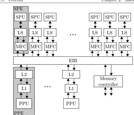
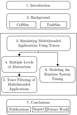
Figure 2.1: The Cell/B.E. microprocessor architecture [100].

Figure 2.1 shows a scheme of the Cell/B.E. microprocessor. It is composed of one general purpose core, called the Power Processor Element (PPE), and eight vector accelerators, each of them called the Synergistic Processor Ele-ment (SPE). The PPE is composed of a two-way SMT in-order 64-bit Power-Architecture [8] core, called the Power Processing Unit (PPU), with 64 KB of L1 cache (32 KB for instructions plus 32 KB for data) and 512 KB of L2 cache.

(33)

2.1. CellSim Chapter 2. Background Both levels of cache are private to the PPE. The PPE executes the operating system and acts as a controller of the eight SPEs.

An SPE includes a SIMD processing core, called the Synergistic Processing Unit (SPU), a 256 KB local memory called Local Store (LS), and a direct-memory-access (DMA) engine called the Memory Flow Controller (MFC). The SPU is a two-wide-issue in-order core with a new SIMD-based instruction set architecture (ISA) [12]. It incorporates just SIMD execution units and has sim-ple hint-based branch prediction because it targets energy efficiency for regular data-intensive codes. The SPU can only access data in the LS. The LS works as an scratchpad memory. To move data in and out of the scratchpad memory, it must be done using DMA commands in the MFC.

The eight SPEs and the PPE are connected using a three-ring intercon-nection network called the Element Interconnect Bus (EIB). The EIB also gave access to off-chip memory through the on-chip memory controller and to off-chip devices through the input/output (I/O) controller.

Both implementations of the Cell/B.E. were clocked at 3.2 GHz and provided a peak single-precision floating-point performance of 204.8 GFLOPS using all eight SPEs. The PowerXCell 8i included, unlike its predecessor, fully-pipelined double-precision floating-point units in the SPEs that provided 102.4 GFLOPS up from 12.8 GFLOPS in the first implementation. These facts confirmed how, although the first implementation of the Cell/B.E. targeted multimedia com-puting, for which double-precision floating-point is irrelevant, the interest of the scientific community led to a second implementation providing full-fledged double-precision floating-point capabilities.

However, the Cell/B.E. architecture also has some weaknesses. Program-ming to achieve high performance is tedious. The non-coherent nature of the LSs requires explicit data movement and the SIMD nature of the SPEs requires programming with vector data structures and deal with alignment, gathering and scattering of data while using close-to-assembler semantics. These pro-grammability limitations added to the high design and development costs that led to its discontinuation.

2.1.2 CellSim Design

Our approach to simulating the Cell/B.E. was to use a modular infrastructure. Using a monolithic approach, apart from being generally bad software engineer-ing practice, would lead to many dependencies among architecture components. Having a modular infrastructure allows having encapsulated components with a clear interface among them. For this purpose, we employed the UNISIM in-frastructure [20] that allows to describe an architecture by specifying a set of modules and the connections among them.

In CellSim, the PPU, caches, SPU, LS, MFC, EIB and memory controller are independent modules. Figure 2.2 shows a scheme of CellSim including its modules and interconnections. The design allows a configurable number of PPEs and SPEs. This allowed to set up a Cell/B.E. configuration with one PPE and eight SPEs, and also exploring future Cell/B.E. implementations with more PPEs and SPEs.

CellSim is an execution-driven simulator. This implies that it has to support two different ISAs, the 64-bit Power ISA and the SPU ISA. Since the SPU ISA was new, we had to implement it from scratch and almost completely as we need

(34)

SPU

LS

MFC

EIB

SPU

LS

MFC

Memory

controller

L2

L1

PPU

PPE

L2

L1

PPU

...

SPE

...

SPU

LS

MFC

SPU

LS

MFC

SPU

LS

MFC

SPU

LS

MFC

Figure 2.2: The CellSim simulator.

to cover around 75% of the instructions for the applications used for evaluation. The PPE works in system-call emulation mode. System calls are emulated by forwarding them to the native operating system running in the host. This implied there is no simulation of the operating system and thus there is no simulation of I/O devices, as shown in Figure 2.2.

The PPU pipeline model was simple, as our focus was on modeling the per-formance of the SPEs, which is the relevant processing component for HPC applications. The SPU pipeline model included a configurable number of exe-cution units and a configurable issue width. The LS had configurable latency and allowed simultaneous access to different banks from the SPU and MFC. The MFC DMA engine was also modeled in detail to account for configurable processing delays, data transfer rates, packet sizes and transfer synchronizations. We performed a functional validation of the PPU and SPU modules and a performance validation of the interconnection network [147, 51].

2.1.3 Lessons Learned

The main problem of CellSim is that it is slow for simulating large configurations. The largest configurations we simulated included 16 SPEs. This is due mainly to three facts:

• Module communication overhead. Modularity brings a set of benefits such as encapsulation and reusability. For example, our module cache served both as L1 and L2 cache. However, one must be careful with the complexity of module communications. UNISIM states a complex

(35)

2.1. CellSim Chapter 2. Background communication protocol between modules. The sender module writes the data in the output port at the beginning of the cycle. Then, the receiving module accepts it or rejects it. If the receiver accepts it, then the sender can enable it or not. This three-way protocol unnecessarily complicates communication and introduces a large overhead for every interconnection port every cycle.

• Software emulation. Due to the execution-driven nature of CellSim, instructions must be functionally simulated (emulated). This has some benefits as we explain in Section 2.3. From a developer’s point of view, implementing the instruction set functionality provides a deep understand-ing of the core features and capabilities. However, from a performance-prediction perspective, emulation adds a simulation overhead for every instruction, something that seems unnecessary if the objective is just to determine the instruction timing.

An additional problem of execution-driven simulation appears when the model is tied to the ISA. In the case of CellSim, the SPU ISA was spe-cific to the Cell/B.E. This restricted the flexibility of CellSim. When the Cell/B.E. was discontinued, software development for the Cell/B.E. stopped and we found ourselves with a restricted amount of applications to feed our simulator with.

In modern execution-driven simulators, functional simulation is decoupled from the timing model. The functional simulation component translates the instructions to an intermediate ”ISA-independent” representation that is fed to the timing model. This way multiple ISAs can be supported and the timing model becomes ISA independent [36].

• Detailed modeling. The use of execution-driven simulation allows a detailed modeling of the processing cores because all the information about the running instruction is available for the timing model. This is useful for detailed modeling of a specific core. However, when that detailed model is replicated for a large number of cores, simulation speed (cycles per second) drops dramatically (typically super linearly). Some of our experiments focused on the interconnect and off-chip memory bandwidth with an increasing number of SPEs. In these cases, most of the time was spent in the detailed modeling of the SPU and LS, while our exploration was not focused in those components. Also, for interconnect and memory bandwidth studies, it is interesting to find the sweet spot design that best manages contention with an increasing number of cores. However, simulating more than sixteen SPEs using such detailed models required long simulation times. As an example, simulations of sixteen SPEs and one PPE using CellSim run at approximately 9 kilo cycles per second (140 kilo instructions per second (KIPS)) on a Pentium 4 at 3 GHz. This is a slowdown of 33 333x compared to native execution.

The lessons learned from these experiences are the following:

• Keep modules communication simple. Modularity provides benefits in terms of clean and structured code, encapsulation and reusability. How-ever, the communication protocol among modules must be simple: enough to do the job with the minimum performance overheads.

(36)

• Keep the timing model ISA independent. Functional simulation in execution-driven simulation must be decoupled from the timing model and an intermediate representation must be used for this to be ISA inde-pendent.

• Use the appropriate modeling detail for each component. The components modeled in detail must be those to which the analysis is tar-geted to. Depending on the type of studies, parts of the timing model may be abstracted to gain simulation speed at the expense of some accuracy loss in the not-so-relevant components. For example, for interconnect, cache hierarchy and memory studies, the model of the processing core, which is the most time-consuming part of the model, can be abstracted. This allows researchers to scale their simulations to larger numbers of cores.

2.2 TaskSim

After the discontinuation of CellSim, we decided to develop a new simulation framework from scratch with the objective of keeping the strengths and get rid of the weaknesses of CellSim.

First, we developed a simulation engine, referred to as CycleSim, to replace UNISIM. From our experience with CellSim, we learned that modularity gives flexibility, encapsulation and reusability, so CycleSim is also based on modules. However, one of the issues in UNISIM was the complexity of the communication protocol between modules, so we simplify it and went from a three-step to an up-to-two-step protocol.

The simulation procedure is similar as with UNISIM, but we redesigned it for speed. UNISIM executes all modules every cycle and all connections must be set every cycle. In CycleSim, we only execute those modules that need to be executed in a given cycle, and even skip empty cycles in which no module has scheduled activity.

Using CycleSim, we developed a set of modules to model the components in multi-core architectures. These modules are then glued together and configured to compose the target architectures of interest.

The CycleSim simulation engine, the modules and the configurations us-ing those modules compose the simulation framework we refer to as TaskSim. TaskSim has been used to carry out a variety of research studies (see Section 7.2) and is the platform on which we have incorporated and evaluated the simulation methodologies and techniques proposed in this thesis.

In the following sections we provide more details on the CycleSim engine, and the modules and configurations we have simulated with TaskSim.

2.2.1 CycleSim

CycleSim allows to describe an architecture using a set of modules and their interconnections. Figure 2.3 shows a producer-consumer communication exam-ple between modules using CycleSim. A Producer module sends some data to a consumer module using the connection at the top of the figure that connects theout port in Producer to thein port in Consumer. Consumer has a queue to store that data until it can be processed due to its processing latency. Then,

(37)

2.2. TaskSim Chapter 2. Background

Producer

Consumer

out in

in out

busy

Figure 2.3: Producer-consumer module example using CycleSim.

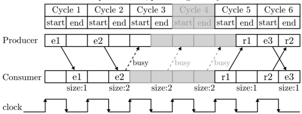
Cycle 1 start end Cycle 2 start end Cycle 3 start end Cycle 4 start end Cycle 5 start end Cycle 6 start end Producer Consumer

e1

clock

e2

size:1 size:2

queue size: 2, processing latency: 3

busy busy busy

r1

r2

e3

e1

e2

r1

r2

e3

size:2 size:2 size:1 size:1

Figure 2.4: Example of communication between Producer and Consumer mod-ules in CycleSim.

when the Consumer queue gets full, it has to notify the Producer to stop it from sending more data that it could not fit in the queue. For this kind of situations, CycleSim provides thebusy signal. The busy signal is generally associated to a interconnection for data, and serves to notify whether the receiving module is ready for processing the data, or is busy and cannot process it. In the example, the Consumer module can set the busy signal so the Producer module does not send more data until the busy signal is unset.

After processing the data, the Consumer module sends the result to the Producer through the interconnection shown in the bottom of the figure. This interconnection does not need a busy signal because the Producer module is at any time ready to process that communication.

As previously mentioned, UNISIM requires all signals to be set every cycle, including the data in the sender module, the acceptance in the receiver module and the enabling of the data in the sender module. Contrarily to UNISIM, in CycleSim, the signals between modules does not necessarily have to be set every cycle, and the busy signal is optional. This results in a much lower overhead per cycle.

Also, in UNISIM, all cycles must be simulated. CycleSim, however, only simulates a module if it has some activity in that cycle or if a signal in its input ports changed. Cycles where no module has activity are skipped, similar to the operation of event-driven simulators.

(38)

ex-ample shown before. In this exex-ample, the Consumer module has a queue that can hold two elements, and it takes three cycles to process the element and send back a response. By convention, modules send data at the start of the cycle, and set/unset their busy signal at the end of the cycle. In the figure, we show the number of elements in the Consumer queue at the end of each cycle.

In the first two cycles, the Producer module sends two elements to the Con-sumer and its queue gets full. The ConCon-sumer then sets the busy signal, and notifies that it does not have to do anything until Cycle 5. In Cycle 3, the Producer reads the busy signal, and notifies that it will not have anything to do until that signal changes or it receives any other data. Therefore, the Consumer module is not executed again until Cycle 5, when it sends back the response to element e1, and the Producer module awakes to handle it. In Cycle 6, the busy signal is not set, the Producer module then sends a third element, and the Consumer sends back the response to element e2.

With this operation, in Cycle 3 the Consumer module was not executed and the Producer only for half cycle. Cycle 4 was never simulated, and in Cycle 5 the Producer only simulates the end of the cycle. The cycles not simulated are shown in grey in the figure.

This implementation allows simulations scalable to large numbers of cores. This is because the number of cycles to be simulated does not determine simu-lation time, but simusimu-lation time is determined by the activity to be simulated in the modeled components.

2.2.2 Modules and Configurations

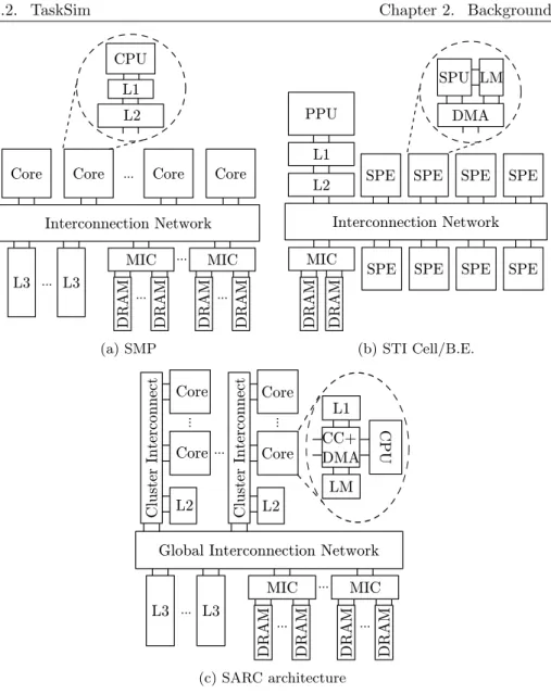
Using the CycleSim semantics, we implemented a set of modules to model cores, caches, local memories, DMA engines, memory controllers, off-chip memory modules and interconnects. This set of modules is used to compose different architectures, thus demonstrating one of the benefits of modularity: reusability. Figure 2.5 shows three examples of target architectures depicted in terms of modules and their interconnections. The first case, in Figure 2.5a, is an SMP configuration with three levels of cache, with a configurable number of cores, L3 cache banks, memory controllers and memory modules.

The configuration in Figure 2.5b models the Cell/B.E. microprocessor (see Section 2.1.1). In this configuration, the L1 and L2 caches are configured to mimic the ones available for the Cell/B.E. PPU, the interconnection network module is adapted to provide the same bandwidth and latency as the Element Interconnect Bus, the scratchpad memory (LM) modules are configured as Local Stores, and the DMA engine module is modified to work as the Memory Flow Controller.

The third example, in Figure 2.5c, is the SARC project architecture [141]. A two-level hierarchical network connects the computation cores in the system to a three-level cache hierarchy and a set of memory controllers giving access to off-chip memory. The several last-level cache (L3) banks are shared among all cores, and data is interleaved among them to provide maximum bandwidth. The L2 banks are distributed among different core groups (clusters) and their data placement policy can be configured to optimize either for latency (data replication), or bandwidth (data interleaving) [170]. Each core has access both to a first-level cache (L1), and to a scratchpad memory (LM). To have determin-istic quick access to data, applications may map a given address range to the

(39)

2.2. TaskSim Chapter 2. Background

Core Core ... Core Core

Interconnection Network MIC DRAM DRAM ... MIC DRAM DRAM ... L3 ... L3 ... L2 CPU L1 (a) SMP Interconnection Network PPU L1 L2

SPE SPE SPE SPE DMA SPU LM

SPE SPE SPE SPE

MIC

DRAM DRAM

(b) STI Cell/B.E.

Global Interconnection Network MIC DRAM DRAM ... MIC DRAM DRAM ... L3 ... L3 Cluster Interconnect L2 Core Core ... Cluster Interconnect L2 Core Core ... ... CC+ DMA CPU LM L1 ... (c) SARC architecture

Figure 2.5: Examples of architectures modeled using TaskSim.

LM, thus avoiding cache coherence issues. A mixed cache controller and DMA engine manages both memory structures (L1 and LM), and address translation. In TaskSim, the modeling effort is devoted to the memory system modules (cache hierarchy, scratchpad memories and off-chip memory), and interconnec-tion network. We model these components in detail and, in contrast, abstract the core model. This is due to two reasons:

• The focus of our research is in macroarchitectural studies regarding the memory system, multi-core density and multi-core organization.

• A detailed modeling of the core pipeline operation is one of the main performance limiting factors in terms of simulation speed due to its costly operation [108].

Raising the level of abstraction : simulation of large chip multiprocessors running multithreaded applications