Proof Complexity of Systems of (Non-Deterministic) Decision Trees and Branching Programs

(Non-Deterministic) Decision Trees and

Branching Programs

Sam Buss

Dept. of Mathematics, UC San Diego, USA https://www.math.ucsd.edu/~sbuss/ [email protected]

Anupam Das

Dept. of Computer Science, University of Copenhagen, Denmark [email protected]

Alexander Knop

Dept. of Mathematics, UC San Diego, USA https://alexanderknop.github.io/ [email protected]

Abstract

This paper studies propositional proof systems in which lines are sequents of decision trees or branching programs, deterministic or non-deterministic. Decision trees (DTs) are represented by a natural term syntax, inducing the system LDT, and non-determinism is modelled by including disjunction, _, as primitive (system LNDT). Branching programs generalise DTs to dag-like structures and are duly handled by extension variables in our setting, as is common in proof complexity (systems eLDT and eLNDT).

Deterministic and non-deterministic branching programs are natural nonuniform analogues of log-space (L) and nondeterministic log-space (NL), respectively. Thus eLDT and eLNDT serve as natural systems of reasoning corresponding to L and NL, respectively.

The main results of the paper are simulation and non-simulation results for tree-like and dag-like proofs in LDT,LNDT,eLDT and eLNDT. We also compare them with Frege systems, constant-depth Frege systems and extended Frege systems.

2012 ACM Subject Classification Theory of computationÑComputational complexity and cryp-tography

Keywords and phrases proof complexity, decision trees, branching programs, logspace, sequent calculus, non-determinism, low-depth complexity

Digital Object Identifier 10.4230/LIPIcs.CSL.2020.12

Related Version A full version of the paper is available at [5],https://arxiv.org/abs/1910.08503.

Funding Sam Buss: This work supported in part by Simons Foundation grant 578919.

Anupam Das: This work was supported by a Marie Skłodowska-Curie fellowship,Monotonicity in Logic and Complexity, ERC project 753431.

1

Introduction

Propositional proof systems are widely studied because of their connections to feasible complexity classes and their usefulness for computer-based reasoning. The first connections to computational complexity arose largely from the work of Cook and Reckhow [11, 16, 17], showing a connection to the NP-coNP question. These results, building on the work of Tseitin [33] initiated the study of the relative efficiency of propositional proof systems. The present paper is introduces propositional proof systems that are closely connected to log-space (L) and nondeterministic log-space (NL).

Our original motivation for this study was to investigate propositional proof systems corresponding to the first-order bounded arithmetic theories VL and VNL for L and NL, see [15]. This follows a long line of work defining formal theories of bounded arithmetic that correspond to computational complexity classes, as well as to provability in propositional proof systems. The first results of this type were due (independently) to Paris and Wilkie [30] who gave a translation from I∆0to constant-depth Frege (AC0-Frege) proofs and to Cook [11] who gave a translation from PV to extended Frege (eF) proofs. Since the first-order bounded arithmetic theory S12 is conservative over the equational theory PV, Cook’s translation also applies to the bounded arithmetic theory S1

2 [7]. As shown in the table below, similar propositional translations have since been given for a range of other theories, including first-order, second-order and equational theories.

Formal Propositional Complexity Theories Proof Systems Class

PV, S1 2 eF P [11, 7] PSA, U1 2 QBF PSPACE [18, 7] Ti2, Si2`1 Gi, G˚i`1 P Σp_i [27, 28, 7] VNC0 Frege (F) ALogTime [14, 15, 1] VL GL˚ _{L [31, 15]} VNL GNL˚ _{NL [32, 15]}

For an introduction to these and related results, see the books [7, 15, 25, 26]. A hallmark of the table above is that the lines in the propositional proofs express (nonuniform) properties in the corresponding complexity class. For instance, lines in a Frege proof are propositional formulas, for which the evaluation problem is complete for alternating log-time (ALogTime), cf. [8]. Likewise, lines in an eFproof are (implicitly) Boolean circuits, for which the evaluation problem is complete for P, cf. [29].

This paper’s main goal is to define alternatives for the proof systems GL˚ and GNL˚ corresponding to log-space and nondeterministic log-space (see [31, 32, 12, 13]). GL˚_restricts cut formulas to be “ΣCNFp2q” formulas; the subformula property then implies that proofs contain only ΣCNFp2qformulas when proving ΣCNFp2qtheorems. GNL˚ _{similarly restricts} cut formulas to be “ΣKrom” formulas.1 ΣCNFp2q and ΣKrom do have expressive power equivalent to nonuniform L and NL respectively [22, 19], but they are are somewhat ad hoc classes of quantified formulas, and their connections to L and NL are indirect. In this paper, we propose new proof systems, eLDT and eLNDT, as alternatives for GL˚ and GNL˚ _{respectively. The lines in eLDT and eLNDT proofs are sequents of formulas} expressingbranching programsandnondeterministic branching programs, respectively. This follows an earlier unpublished suggestion of S. Cook [10], who gave a system for L based on branching programs via “Prover-Liar” games (see [9]). The advantage of our systems is that deterministic and nondeterministic branching programs correspond directly to nonuniform L and NL respectively and do not require the use of quantified formulas. (See [34] for a comprehensive introduction to branching programs.)

1 _{A ΣKrom formula has the form if it has the formD~zφp~z, ~xq, whereφis a conjunctionC}

1^C2^ ¨ ¨ ¨ ^Cn

To design the proof systems eLDT and eLNDT, we need to choose representations for branching programs. For this, we use a formula-based representation, as this fits well into the customary frameworks for proof systems. Since formulas only represent tree-structures, we first define the systems LDT and LNDT for decision trees and non-deterministic decision trees, respectively. From here dag-like structures are described using extension variables, allowing us to abbreviate complex formulas by fresh variables, yielding the systems eLDT and eLNDT. An example this is given in Figure 2 on page 12. This is similar to the way the extension variables in extended Frege proofs allow circuits to be expressed by small formulas.

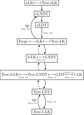
We start in Section 2 describing proof systems LDT and LNDT that work with just deterministic and nondeterministic decision trees (without extension variables). Deterministic decision trees are represented by formulas using a single “case” or “if-then-else” connective, written in infix notationApB, which means “ifpis false, thenA, elseB”. The conditionpis required to be a literal, butAandB are arbitrary formulas. The system LDT is a sequent calculus system in which all formulas are decision trees. Nondeterministic decision trees may further be composed by disjunctions, allowing formulas of the formpA_Bq. The system LNDT is a sequent calculus in which all formulas are nondeterministic decision trees. LDT and LNDT are weak systems; in fact, they are both polynomially simulated by depth-2 LK that is, by the sequent calculus LK with all formulas are depth two, allowing proofs to be dag-like. Figure 1 shows the equivalences between systems as currently established; those that concern LDT and LNDT are given in Section 4. Section 5 introduces the proof systems eLDT and eLNDT for branching programs and nondeterministic branching programs.

One issue in designing these proof systems is the treatment of isomorphic or bisimilar branching programs. One approach is to allow proofs to freely replace any branching program with any isomorphic or bisimilar branching program by means of additional axioms, e.g. as done by Jeřábek [21] for the reformulation of extended Frege using Boolean circuits as lines. The problem with using isomorphism or bisimilarity axioms is that these problems (for branching programs) are in NL but not known to be in L. Such axioms are thus undesirable, at least for eLDT, as it is a proof system for log-space. We instead adopt a more conservative approach: the equivalence of bisimilar branching programs must be proved explicitly.

Since formulas in eLDT and eLNDT proofs express nonuniform L and NL properties, respectively, they are intermediate in expressive power between Boolean formulas (expressing NC1 properties) and Boolean circuits (expressing nonuniform P properties). Thus it is not surprising that, as shown in Figure 1, these two systems are between Frege and extended Frege in strength. In addition, since NL properties can be expressed by quasipolynomial size formulas, it is not unexpected that Frege proofs can quasipolynomially simulate eLNDT, and hence eLDT. These results are given in Section 6.

We include only brief proof sketches in this paper, due to space constraints, but full proofs may be found in [5].

2

Decision tree formulas and

LDT

proofs

This section describes decision tree (DT) formulas, and the associated sequent calculus proof system LDT. All our proof systems arepropositional proof systems with variablesx, y, z . . . intended to range over the Boolean valuesFalse andTrue. We use 0 and 1 to denote the constants False andTrue, respectively. Aliteral is either a propositional variablexor a negated propositional variablex. We use use variablesp, q, r, . . .to range over literals.

The only connective for forming decision tree formulas (DT formulas) is the 3-ary “case” function, written in infix notation aspApBqwhereAand B are formulas andpis required to be a literal. This informally means “ifpis false, thenA, elseB”. Formally:

Tree-1-LK Tree-LDT Tree-2-LK

_ÐÑ

Thm 18 Tree-LNDT

_ÐÑ

Thm 17 LDTThm 13

_ÐÑ

Thm 14 1-LK 2-LK

ÐÑ

Thm 18 LNDT Frege

ÐÑ

LK

ÐÑ

Tree-LK eLDT eLNDT eLK

ÐÑ

Tree-eLK Thm 13 qp Thm 14 Thm 29 qp Thm 30

Figure 1 Relations between proof systems. Ñmeans “polynomially simulates”; Ñqp means

“quasipolynomially simulates”;99Kmeans “exponentially separated from”. d-LK is the system of dag-like LK proofs with only depthdformulae occurring (atomic formulae have depth 0) By default, all proof systems allow dag-like proofs, unless they are labeled as “Tree”.

IDefinition 1. Decision tree formulas, or DT formulas, are inductively defined as follows:

1. any literalpis aDT formula, and

2. if AandB areDT formulas andpis a literal, thenpApBq is aDTformula. We callp the decision literalof this formula.

The size of a DTformula Ais the number of occurrences of atomic formulas inA.

Supposeαis a 0-1-truth assignment to the variables; the semantics of DT formulas is defined by extendingαto be a truth assignment to all DT formulas by inductively defining:

αpxq “ 1´αpxq (1)

αpApBq “

#

αpAq ifαppq “0 αpBq otherwise.

It is important that onlyliterals pserve as the case distinctions in DT formulas. Notably, forC a complex formula, an expressionpA C Bq, which evaluates toA ifC is true and toB ifC is false, would in general denote a decisiondiagramrather than a decision tree.

Although there is no explicit negation of DT formulas, we informally define the negation Aof a DT formula inductively by lettingxdenotex, and lettingApB denote the formula A p B. Of courseA is a DT formula wheneverA is, andAcorrectly expresses the negation ofA. Notice also that negative decision literals are “syntactic sugar”, sinceApB¯ is equivalent toBpA. Nonetheless the notation is useful for making later definitions more intuitive.

Our definition of DT formulas is somewhat different from the usual definition of decision trees. The more common definition would allow 0 and 1 as atomic formulas instead of literalspas in condition 1 of Definition 1. We call such formulas 0{1-DT formulas; they are equivalent to DT formulas in expressive power. The constants 0 and 1 are equivalent toppp andppp, for any literalp. More generally, 0pA, 1pA,Ap0 orAp1 are equivalent toppA,ppA, App, or App, respectively. Conversely, a literalp, when used as atom, is equivalent to 0p1.

IRemark 2 (Expressive power of decision trees). It is easy to decide the validity or satisfiability of a DT formula with a log-space algorithm. To check satisfiability, for example, one examines each leaf in the formula tree (each atomic subformulap) and verifies whether the path of literals from the root to the leaf is consistent with some truth assignment.

A DT formulaAof sizencan be expressed as a DNF formula of sizeOpn2qwith at most n disjuncts, defined formally in Section 3. Informally this DNF is formed by taking the disjunction of terms (a.k.a conjunctions of literals) corresponding to paths from the root to a leaf. A dual construction expresses a DT formulaA as a CNF formula of sizeOpn2

qwith at most nconjuncts. It is folklore that the construction can be partially reversed: namely any Boolean function that is equivalently expressed by a DNFϕand a CNFψcan be represented by a DT formula of size quasipolynomial in the sizes ofϕandψ. This bound is optimal, as [23] proves a quasipolynomial lower bound.

We next define the proof system LDT for reasoning about DT formulas. Lines in an LDT proof are sequents, hence they express disjunctions of DT’s. Thus lines in LDT proofs can express DNF properties, whose validity problem is non-trivial, indeed coNP-complete.

IDefinition 3. Acedent, denotedΓ,∆etc., is a multiset of formulas; we often use commas for multiset union, and writeΓ, Afor the multisetΓ,tAu. Asequentis an expressionΓ

Ñ

∆ whereΓ and∆ are cedents. Γ and∆are called the antecedentand succedent, respectively. The intended meaning of Γ

Ñ

∆ is that if every formula in Γ is true, then some formula in ∆ is true. Accordingly, Γ

Ñ

∆ is true under a truth assignmentαiffαpAq “0 for someAPΓ orαpAq “1 for someAP∆. A sequent isvalid iff it is true for every truth assignment.

IDefinition 4. The sequent calculus LDTis a proof system in which lines are sequents of DT formulas. The valid initial sequents (axioms) are, forpany literal,

p

Ñ

p p, p

Ñ

Ñ

p, p.

The rules of inference are:

Contraction rules: c-l: A, A,Γ

Ñ

∆ A,Γ

Ñ

∆ Γ

Ñ

∆, A, A c-r: Γ

Ñ

∆, A Weakening rules: w-l: Γ

Ñ

∆ A,Γ

_Ñ

∆ Γ

Ñ

∆ w-r: Γ

_Ñ

∆, A

Cut rule: cut: Γ

Ñ

∆, A A,Γ

Ñ

∆

Γ

Ñ

∆

Decision rules: dec-l: Γ, A

Ñ

p,∆ Γ, p, B

Ñ

∆ Γ, ApB

Ñ

∆

Γ

Ñ

A, p,∆ Γ, p

Ñ

B,∆ dec-r:

Proofs are, by default, dag-like. I.e. a proofof a sequentS inLDTis a sequencepS0, . . . , Snq such thatS isSn and eachSk is either an initial sequent or is the conclusion of an inference step whose premises occur amongstpSiqiăk. The subsystem where proofs are restricted to be tree-like (i.e. trees of sequents composed by inference steps) is denoted Tree-LDT.

The size of a proof is the sum of the sizes of the formula occurrences in the proof. The inference rules that are new to LDT are the two decision rules,dec-l and dec-r. Since ApB is equivalent topA_pq ^ pp_Bq, the lower sequent of a dec-r is true (under some fixed truth assignment) iff both upper sequents are true under the same assignment, i.e. the rule is sound and invertible. Similarly, sinceApB is also equivalent topA^pq _ pp^Bq, the dec-l rule is also sound and invertible.

IRemark 5 (Cut-free completeness). The invertibility properties also imply that the cut-free fragment of LDT is complete. To prove this by induction on the complexity of sequents, start with a valid sequent Γ

Ñ

∆; choose any non-atomic formulaApB in Γ or ∆, and apply the appropriate decision ruledec-l ordec-r that introduces this formula. The upper sequents of this inference are also valid and, furthermore, they have logical complexity strictly less than the logical complexity of Γ

Ñ

∆. The base case of the induction is when Γ

Ñ

∆ contains only atomic formulas; in this case, it can be inferred from an initial sequent with weakenings. Note that this shows in fact, that any valid sequent can be proved in LDT using only decision rules, weakenings, and initial sequents. The system also enjoys a “local” cut-elimination procedure, via standard techniques, but that is beyond the scope of this work.

IProposition 6. The following have polynomial size, cut-free, Tree-LDTproofs:

(a) A

Ñ

A (b)

Ñ

A, A (c) A, A

Ñ

(d) A

Ñ

p, ApB (e) p, B

Ñ

ApB (f ) ApB

Ñ

A, p (g) ApB, p

Ñ

B

3

Comparing

DT

proof systems and

LK

proof systems

LK is the usual Gentzen sequent calculus for Boolean formulas over the basis^and_. The Boolean formulasare defined inductively by

Any literalpis a Boolean formula, and

IfAandB are Boolean formulas, then so arepA_BqandpA^Bq.

The proof system LK has the same initial sequents (axioms) as LDT, its inference rules are the contraction rulesc-l andc-r, the weakening rules w-l and w-r, the cut rule, and the following Boolean rules:

A, B,Γ

Ñ

∆ ^-l: A^B,Γ

Ñ

∆ Γ

Ñ

∆, A Γ

Ñ

∆, B ^-r: Γ

Ñ

∆, A^B A,Γ

_Ñ

∆ B,Γ

_Ñ

∆ _-l: A_B,Γ

Ñ

∆ Γ

_Ñ

∆, A, B _-r: Γ

Ñ

∆, A_B

Recall that aclause is a disjunction of literals and aterm is a conjunction of literals.

IDefinition 7. A Boolean formula is depth one if it is either a clause or a term. 1-LK is the fragment ofLKin which all formulas appearing in sequents are depth one formulas. Tree-1-LKis the same system with the restriction that proofs are tree-like.

If~pis a vector of literals, we writeŽ

~

pto denote a disjunction of the literals ~p, taken in the indicated order. The notationŹ

~

pis defined similarly. The nesting of disjunctions and conjunctions can be arbitrary, soŽ~pdenotes any formula of the formpŽp~1_{q _ p}Ž

~

~

p1 _and~p2 _{denotep1, . . . , pk andpk}

´1, . . . , p` for some 1ďkď`. Although these notations are ambiguous about the nesting of disjunctions or conjunctions, this makes no difference in this work, since ifAandB are both of the formŽ

~

pbut with different orders of applications of_’s, then there are polynomial size, cut-free Tree-1-LK proofs ofA

Ñ

B andB

Ñ

A.

Later theorems will compare the proof theoretic strengths of various fragments and extensions of LDT to fragments of LK. Since these theories use different languages, we need to establish translations between cedents of DT formulas and (depth one) Boolean formulas.

IDefinition 8. For a (nonempty) sequence of literals ~pwe define the DT formulasConjp~pq andDisjp~pqby induction on the length of ~pas follows:

Conjppq :“ p

Conjpp, ~pq :“ pppConjp~pqq

Disjppq :“ p

Disjpp, ~pq :“ pDisjp~pqppq In other words, if ~p“ pp1, . . . ,p`q, for`ą1, we have:

Conjpp~q “ pp1p1pp2p2p¨ ¨ ¨ pp`´2p`´2pp`´1p`´1p`qq ¨ ¨ ¨ qqq Disjpp~q “ ppp¨ ¨ ¨ ppp`p`´1p`´1qp`´2p`´2q ¨ ¨ ¨ qp2p2qp1p1q.

It is not hard to verify that Conj and Disj correctly express the conjunction and disjunction of the literals~p. This is borne out by the next proposition.

IProposition 9. The following sequents have polynomial size, cut-freeTree-LDT proofs.

(a) Conjp~p, ~qq

Ñ

Conjp~pq

(b) Conjp~p, ~qq

Ñ

Conjp~qq

(c) Conjp~pq,Conjp~qq

Ñ

Conjp~p, ~qq

(d) Disjp~pq

Ñ

Disjp~p, ~qq

(e) Disjp~qq

Ñ

Disjp~p, ~qq

(f ) Disjp~p, ~qq

Ñ

Disjp~pq,Disjp~qq

For the converse direction of simulating LDT (and its supersystems) by LK, we need to express DT formulasAas Boolean formulas in both CNF and DNF forms. For this we define TmspAqas a multiset of terms (i.e., a multiset of conjunctions) and ClspAqas a multiset of clauses (i.e., a multiset of disjunctions) so thatA is equivalent to both the DNFŽTmspAq and the CNFŹ

ClspAq.

IDefinition 10. LetA be a DT-formula. The terms and clauses of A are the multisets TmspAqandClspAqinductively defined by lettingTmsppqandClsppqboth equalp, and letting TmspBpCq :“ tpp^Dq:DPTmspBqu Y tpp^Dq:DPTmspCqu (2) ClspBpCq :“ tpp_Dq:DPClspBqu Y tpp_Dq:DPClspCqu. (3) For example, ifAisp1p2pp3p4p5qthen TmspAqistp2^p1, p2^p4^p3, p2^p4^p5u,and ClspAqis equal totp2_p1, p2_p4_p3, p2_p4_p5u.

The equivalence between A,Ž

TmspAqand Ź

ClspAqis witnessed by simple proofs:

IProposition 11. There are polynomial size, cut-freeTree-LK-proofs of:

(a) C

Ñ

D, for eachCPTmspAqandDPClspAq.

(b) (i) ClspApBq

Ñ

D, p, for each DPClspAq;

(ii) p,ClspApBq

Ñ

D, for each DPClspBq.

(iii) ClspAq

Ñ

D, p, for eachDPClspApBq.

(iv) p,ClspBq

Ñ

D, for each DPClspApBq.

(c) (i) C

Ñ

p,TmspApBq, for each CPTmspAq;

(iii) C

Ñ

p,TmspAq, for each CPTmspApBq.

(iv) p, C

Ñ

TmspBq, for each CPTmspApBq.

Proof sketch. Part (a) of the lemma is proved by induction on the complexity ofA. Parts (b) and (c) are trivial once the definitions are unwound. For example, (b.i) follows from the fact that ClspApBqcontains the formula p_D. This allows (b.i) to be derived from the two sequentsp

Ñ

pandD

Ñ

D. The former is an axiom, and the latter has a tree-like cut-free proof by Proposition 6a. The other cases are similar. _J The next definition shows how to compare proof complexity between proof systems that work with DT formulas and ones that work with Boolean formulas.

IDefinition 12. Let P be a proof system for sequents of Boolean formulas (or at least, sequents of depth one Boolean formulas), andQbe a proof system for sequents of DT formulas. We say thatP polynomially simulates Qif there is a polynomial time procedure which, given aQ-proof of

A0, . . . , Am´1

Ñ

B0, . . . , Bn´1, (4)

where theAi’s andBi’s are DT-formulas, produces a P-proof of

ClspA0q, . . . ,ClspAm´1q

Ñ

TmspB0q, . . . ,TmspBn´1q. (5) The system Qpolynomially simulatesP if there is a polynomial time procedure which, given aP-proof of ł ~a0, . . . , ł ~am´1

Ñ

ľ ~b0, . . . , ľ ~bn´1, (6)

where the~ai’s and~bi’s are sequences of literals, produces aQ-proof of

Disjp~a0q, . . . ,Disjp~am´1q

Ñ

Conjp~b0q, . . . ,Conjp~bn´1q. (7) The systems P andQare polynomially equivalentif they polynomially simulate each other. (5) is called theBoolean translationof (4). (7) is called theDT-translationof (6). Quasipoly-nomial simulation and equivalenceare defined in the same way, but using quasipolynomial time (time 2logOp1qn) procedures.2

3.1

1-LK

and

LDT

Our first results compare the weakest systems considered in this work, operating with just DT formulas or with just terms and clauses.

I Theorem 13. LDT polynomially simulates 1-LK. Tree-LDT polynomially simulates Tree-1-LK.

Proof sketch. We may replace terms Ź

~a and clauses Ž

~aoccurring in a 1-LK proof by DT-formulas Conjp~aqor Disjp~aqrespectively. The result can be adapted into a correct LDT

proof using cuts against proofs from Proposition 9. _J

2 _{It turns out that all stated quasipolynomial simulations in this work (Theorems 14 and 30) take time}

nOplognq

“2Oplog2_n

A converse result holds too, but we have only a quasipolynomial simulation in the tree-like case. It is open whether this can be improved to a polynomial simulation.

ITheorem 14. 1-LKpolynomially simulatesLDT. Tree-1-LK quasipolynomially simulates Tree-LDT.

Proof sketch. In a given LDT proof, we may replace every DTAin an antecedent by the multiset ClspAqand every DTAin a succedent by TmspAq. The result can be adapted into a correct 1-LK proof using cuts against proofs of the truth conditions from Proposition 11. In the tree-like case, when simulating the cut rule we must copy one subproof polynomially many times (such copying is unnecessary when proofs are dag-like). However it turns out we may freely choose which of the two subproofs to duplicate, so we may just take the smaller one, which has size at most half that of the original proof. Doing this recursively yields a nOplognq_“2Oplog2_nq

bound on the size of the resulting Tree-1-LK proof. _J

4

Nondeterministic decision tree formulas and

LNDT

proofs

This section defines nondeterministic decision tree (NDT) formulas, and the associated sequent calculus LNDT. The NDT formulas have two kinds of connectives; the 3-ary case functionApBand the Boolean OR-gate (_). Formally:

IDefinition 15. The nondeterministic decision tree formulas, or NDT formulas for short, are inductively defined by

Any literalpis aNDT formula;

If A andB are NDTformulas and pis a literal, thenpApBqis aNDT formula; If A andB are NDTformulas, then pA_Bqis an NDT formula.

A nondeterministic gate in a decision tree accepts just when at least one of its children is accepting. This corresponds exactly to an _gate, which yields True exactly when at least one input is True. One of our motivations in defining LNDT that is will serve as a foundation for our later definition eLNDT, which will capture a logic for nondeterministic branching programs, and hence a logic for nonuniform NL.

IDefinition 16. The sequent calculusLNDTis a proof system in which lines are sequents of NDT formulas. Its initial sequents (axioms) and rules are the sames as those of LDT, along with the two_inferences,_-l and _-r, ofLKas described on page 6.

For αa 0-1-truth assignment, the semantics of NDT formulas is defined extending the definition of the semantics of DT formulas, in equations 1, to include

αpA_Bq “

#

1 ifαpAq “1 orαpBq “1 0 otherwise.

It is straightforward to verify that LNDT is sound and complete for sequents of NDT formulas, by a similar argument to that of Remark 5.

4.1

LDT

and tree-like

LNDT

are equivalent

Next we turn to the relative complexity of LDT and LNDT. Naturally the latter subsumes the former, but this can be strengthened as follows:

We will soon see that this also refines the known polynomial equivalence between 1-LK and Tree-2-LK (see [2, 3]), by virtue of Theorems 14 and 18.

Proof sketch. To show that Tree-LNDT polynomially simulates LDT we notice that lines of an LDT proof (i.e. sequents of DT formulas) may be expressed as NDT formulas. From here one may use an adaptation of a standard technique for showing that tree-like LK is equivalent to dag-like LK, carefully managing the complexity of formulas occurring.

To show that LDT polynomially simulates Tree-LNDT, we first notice that each NDT formula may be written as a disjunction of DT formulas (“normal form”), and further-more that LNDT proofs may be written in a way that operates with only such formu-las with only polynomial blowup. Now we convert a normal form Tree-LNDT proof π of Ž Π1, . . . , Ž Πk

Ñ

Ž Λ1, . . . , Ž

Λl to a (dag-like) LDT derivation π1 of the sequent

Ñ

Λ1, . . . ,Λl from extrahypothesest

Ñ

Πiuki“1. This is proved by induction on the struc-ture of the proof tree and takes polynomial time. Now, whenπderives a DT sequent, notice thatπ1 _{is just a LDT proof of the same sequent.}

J

4.2

Equivalence of

LNDT

and

2-LK

A Boolean formula is depth two if it is depth one, or if it is a conjunction of clauses or a disjunction of terms. 2-LK is the fragment of LK in which all formulas occurring are depth two formulas. Tree-2-LK is the same system with the restriction that proofs are tree-like.

ITheorem 18. LNDTand2-LK are polynomially equivalent. Tree-LNDT andTree-2-LK are polynomially equivalent.

This is not so surprising a result, since NDTs have equivalent expressive power to DNFs, so depth two sequents may be written as NDT sequents and vice-versa.

Proof sketch. A (two-sided) 2-LK proof is simulated in LNDT by simply replacing every DNFŽ i Ź ~ pi with the NDT Ž

iConjp~piqand locally repairing the proof using cuts against proofs from Proposition 8. In the other direction we work with “normal form” LNDT proofs (as in the proof of Theorem 17). From here the translation to DNFs is straightforward, since DT formulas already have small DNFs, cf. Definition 10. Again, we use cuts against proofs of the appropriate truth conditions. Both simulations map tree-like proofs to tree-like

proofs. _J

5

Proof systems for branching programs

5.1

Formulas and proofs with extension variables

We now describe the systems eLDT and eLNDT which reason about deterministic and nondeterministic branching programs respectively.3 Formulas can now include extension variables, usually denoted by e1, e2, etc. It is important that the extension variables are explicitly distinguished from the propositional variables we have thus far used.

The purpose of extension variables is to serve as abbreviations for more complex formulas. Thus, proofs that use extension variables will be accompanied by a set of extension axioms teiØAiuiăn, where each formulaAi may use any literalspbut is restricted to use only the extension variablesej forjăi. The intent is thatei is an abbreviation for the formulaAi.

IDefinition 19. Extended decision treeformulas (eDTformulas) are defined as follows:

(1) Any literalpis an eDTformula.

(2) Any extension variable eis an eDTformula.

(3) If A andB areeDT formulas andpis a literal, then pApBqis aDT formula.

In particular, a decision literalpin a formulaApBisnotallowed to be an extension variable. The intuition is that the extension variables may “name” nodes in a branching program.

IDefinition 20. Extended nondeterministic decision treeformulas (eNDT formulas) are defined by the closure conditions (1)-(3) above (replacing “eDT” by “eNDT”) and:

(4) If A andB areeNDT formulas, thenpA_Bqis aneNDT formula.

A set of extension axioms is a set A“ tei ØAiuiăn where e0, . . . , en´1 are extension variables such that the only extension variables appearing inAi are e0, . . . , ei´1, foriăn. We identifyAwith the set of sequents consisting ofei

Ñ

AiandAi

Ñ

ei, foriăn. eDT and eNDT formulas have truth semantics only relative to a set of extension axiomsteiØAiuiăn. Namely, forαa truth assignment, the definition of truth is extended by settingαpeiq “αpAiq.

I Definition 21. An eLDT proof is a pair pπ,Aq where A “ tei Ø Aiuiăn is a set of extension axioms where eachAi is aneDTformula, and πis anLDTderivation which is allowed to use initial sequents fromA. eLNDT proofs are defined similarly, but witheLNDT formulas Ai andeLNDT derivations.

Note that all formulas in an eLDT or eLNDT proof are based on a single set of extension axiomsteiØAiuiăn.

Let us discuss how the extended formulas we have introduced may be used to represent bona fide branching programs. A (deterministic) branching program is a directed acyclic graphGsuch that (a) Ghas a unique source node, (b) sink nodes in Gare labelled with either 0 or 1, (c) all other nodes are labelled with a literalpand have two outgoing edges, one labelled 0 and the other 1. Gcan be converted into an equivalent eDT formula with associated extension axioms tei ØAiuiăn by introducing an extension variable for every internal node in G. Conversely, as is described in more detail in Section 5.2, any eDT formulaA with extension axiomsteiØAiuiăn can be straightforwardly transformed into a linear size deterministic branching program. For this, the nodes in the branching program correspond to the extension variablesei and the subformulas of the formulasAi.

Nondeterministic branching programs are defined similarly to deterministic branching programs, but further allowing the internal nodes ofGto be labelled with “_” as well as literals (in this case the labelling of its outgoing edges is omitted). The semantics is that an _-node is accepting provided at least one of its children is accepting. It is straightforward to convert a nondeterministic branching program into an eLNDT formula with associated extension axioms, and vice versa. A similar construction yields the folklore fact that “extended Boolean formulas” are as expressive as Boolean circuits.

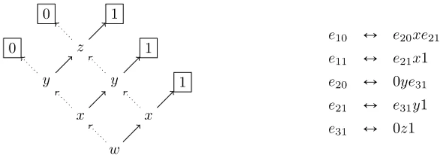
IExample 22. Consider the (deterministic) branching programGin Figure 2, on the left, which returns 1 just if at least two out of the four input variablesw, x, y, z are 1. Edges labelled with 0 are here dotted (and always left outgoing) while edges labelled 1 are here solid (and always right outgoing). In this particular case, the branching program isordered (or anOBDD), i.e. variables occur in the same relative order on each path from the source

to a sink. The program also happens to compute a monotone Boolean function.

To representGin eLDT, we introduce extension variables for each internal node of the program as follows. Write eij for the jth node of the ith layer, with i, j ranging from 0 onward, and introduce the extension axioms in Figure 2, on the right.4 _{Now Gis represented}

w x x y y ₁ 0 z 1 0 1 e10 Ø e20xe21 e11 Ø e21x1 e20 Ø 0ye31 e21 Ø e31y1 e31 Ø 0z1

Figure 2A branching programG, on the left, computing the 2-out-of-4 threshold function and an encoding of its (internal) local conditions by extension variables, on the right. Dotted edges are labelled 0 and solid edges are labelled 1.Gis equivalent to the eDT formulae10we11.

by the eDT formulae10we11. Notice that the orderedness of the program is reflected in its eLDT representation: writingpx0, x1, x2, x3qforpw, x, y, zq, we have thatxi is the root of the formula that anyeij abbreviates.

Other representations ofGare possible, for instance by renaming the extension variables or by partially unwinding the graph. In both these two latter cases, the eDT representation obtained will be provably equivalent to the one above, by polynomial-size proofs in eLDT, by virtue of Lemma 28 later.

5.2

Foundational issues and Boolean combinations

The fact that extension variables cannot be used as decision literals is a significant limitation on the expressiveness of DT formulas. Recall for instance that the conjunction ofp1 andp2 can be expressed with the DT formula Conjpp1, p2q, namely pp1p1p2q. However, it is not permitted to form pe1e1e2q; in fact, it is not possible to express the conjunction e1^e2 without taking the extension axioms defining e1 and e2 into account. If we could write the conjunction of e1 and e2 by a generic formula Ape1, e1q, then we could introduce a new extension variable representing Ape1, e2q. This would imply that eDT formulas are as expressive as extended Boolean formulas; in other words, that deterministic branching programs would be as expressive as Boolean circuits. This is a non-uniform analogue of L“P (i.e., log-space equals polynomial time) and, of course, is an open question.

Nonetheless, for any given extension variables e and e1_{, there is a formula}

Andpe, e1_q expressing the conjunction ofeand e1 _{by changing the underlying set of extension axioms.} The intuition is that we start with the branching programGfore, but now with sink nodes labelled with 0 or 1 instead of with variables. To form the branching program fore^e1_{, we} take (an isomorphic copy) of the branching programG1 _fore1_{, and modifyGby replacing} each sink node labelled with 1 with the source node ofG1_{(in other words, each edge directed} into a sink “1” is modified to instead point to the root ofG1_{). Since we do not actually have} 0 and 1 in the language, we work modulo their encodings by literals:

IDefinition 23. Let C be an eDTor eNDT formula. Cr0{Bs is the formula obtained by replacing (in parallel) each occurrence of a literalpas a leaf inC with the formula pB p pq. Similarly,Cr1{Bsis the formula obtained by replacing each occurrence of a literalpas a leaf inC with the formula pp p Bq.

The point ofCr0{Bs is thatpB p pqevaluates to 1 ifpis true, and to B otherwise. Thus, the intent is thatCr0{Bsis equivalentC_B. Likewise, we wantCr1{Bsto be equivalent

C^B. However, these equivalences hold only if the substitutions are applied not just inC but instead throughout the definitions of the extension axioms used inC. This is done with the following definition.

IDefinition 24. LetAbe a set of extension axiomsteiØAiuiăn. Another set of extension axiomsAr1{Bsis defined as follows. First, lette1

iuibe a set of newextension variables. Define Air~e1_{{~esto be the result of replacing each ej inAi withe}1

j. Let A1i bepAir~e1{~esqr1{Bs. Then Ar1{Bsis the set of extension axiomste1

i ØA1iuiănYA. The setAr0{Bsis defined similarly: letting~e2 _{be another set of new extension variables, definingA}2

i to bepAir~e2{~esqr0{Bs, and letting Ar0{Bsbe the set of extension axioms te2

i ØA2iuiănYA.

Finally, if Aand B areeDToreNDT formulas defined using extension axiomsA, then

AndpA, Bqis by definition Ar1{Bsrelative to the extension axioms Ar1{Bs. The formula

OrpA, Bq for disjunction is defined similarly, namely, it is equal toAr0{Bs relative to the extension axiomsAr0{Bs.

Note the two formulas_AndpA, Bqand_OrpA, Bqintroduceddifferentsets of new extension variables, so we may use both AndpA, Bq and OrpA, Bq without any clashes between extension variables. More generally, we adopt the convention that the new extension variables are uniquely determined by the Boolean combination being constructed. For instance,e1 i could have instead been designated ei,pA^Bq. When measuring proof size, we also need to count the sizes of the subscripts on the extension variables. This clearly however only increases proof size polynomially.

There are two other sources of growth of size in forming _AndpA, Bqand_OrpA, Bq. The first is that formula sizes increase since copies ofBis substituted in at many places inAand A: this potentially gives a quadratic blowup in proof size. We avoid this quadratic blowup in proof size, by always takingB to be a single variable (namely, an extension variable). The construction ofAndpA, BqorOrpA, Bqalso introduces many new extension variables, namely it potentially doubles the number of variables. To control this, we will ensure that the constructions ofAndp¨,¨qandOrp¨,¨qare nested only logarithmically.

IExample 25. Consider the formula _Andpp1,Andpp2, p3qq, which is a translation of the Boolean formula p1^ pp2^p3qto a DT formula. To formAndpp2, p3q, start with pp2p21q and substitutep3 for “1”, to obtain pp2p2p3q. Then _Andpp1,_Andpp2, p3qqis obtained by formingpp1p11qand replacing “1” withAndpp2, p3qto obtainpp1p1pp2p2p3q. It is also the same as Conjpp1, p2, p3q. A similar construction shows that Orpp1,Orpp2, p3qis equal to ppp3p2p2qp1p1q. This is a translation of the Boolean formulap1_ pp2_p3qto a DT formula, and is equal to Disjpp1, p2, p3q.

IExample 26. LetA be the formulapp1p2pe1p3e2qqandB be the formulapq1q2e2qin the context of the extension axiomsA

e1Ø pr1r2e2q e2Ø ps1s2s3q, (8)

wherepi, qi, ri, si are literals. The formula Ar0{Bs is formed as follows. First Ap~e1{~eq is e1

1Ø pr1r2e12q, e12 Ø ps1s2s3q. Then Ar0{Bscontains the extension axioms ofAas shown in (8) plus the extension axioms e1

1 Ø ppBr1r1qr2e12q, e21 Ø ppB s1s1qs2pBs3s3qq. Finally, Ar0{Bsis the DT formula ppBp1p1qp2pe11pe12qq, namely, pppq1q2e2qp1p1qp2pe11pe12qq, relative to the four extension axioms inAr0{Bs.

5.3

Truth conditions and renaming of extension variables

We show that, despite the delicate renaming of variables required for notions such asAr0{Bs and_AndpA, Bq, for DT (respectively eNDT) formulasA, B, we may nonetheless realise their

I Lemma 27. Let A and B be eDT formulas (respectively, eNDT formulas) relative to extensions axiomsA. Then, the sequents(a)-(c) below have polynomial size, cut freeeLDT proofs (respectively,eLNDTproofs) relative to the extension axiomsAr0{Bs. The same holds for the sequents(d)-(f)relative toAr1{Bs.

(a) B

Ñ

Ar0{Bs (b) A

Ñ

Ar0{Bs (c) Ar0{Bs

Ñ

A, B (d) Ar1{Bs

Ñ

B (e) Ar1{Bs

Ñ

A (f ) A, B

Ñ

Ar1{Bs

Proof sketch. Parts (a)-(c) are proved by showing inductively that ifC is a subformula of Ar0{Bsor a subformula of anyA1

iin Ar0{Bs, thenC

Ñ

A, B andB

Ñ

CandA

Ñ

C have short eLDT (resp., eLNDT) proofs. The base cases are just the cases whereC is is the form pB p pq. The inductive cases are trivial. A similar argument proves cases (d)-(f). _J The proofs of Lemma 27 seem to be inherently dag-like, and we do not know if there are polynomial-size Tree-eLDT proofs for those sequents.

As discussed above, we assume that the choice of new extension variables~e1_or~e2_depends explicitly on what formulaAndpA, BqandOrpA, Bqis being formed. In other words, each e1

i or e2i is a variable ei,_AndpA,Bq or ei,_OrpA,Bq. In the proof of Theorem 29 later, this means that the translations of distinct occurrences of the same Boolean formula use the same extension variables. However, this is not strictly necessary, as eLDT can prove the equivalence of formulas after renaming extension variables:

ILemma 28. SupposeA is a DT formula w.r.t. extension axiomsA“ tei ØAiui, and that the extension variables f~are distinct from the extension variables~e. Let B equalArf~{~es w.r.t. the extension axiomsB“ tfiØAirf~{~esui. Then eLDThas a polynomial size, cut free (dag-like) proofs ofA

Ñ

B andB

Ñ

A relative to the extension axiomsAYB.

Lemma 28 has a straightforward proof that proceeds inductively through all subformulas of the formulasAi andA.

6

Simulations for

eLDT

,

eLNDT

and

LK

We compare the systems eLDT and and eLNDT with LK, showing that they are all quasi-polynomially related in terms of proof size, constituting the upper half of Figure 1.

6.1

eLDT

polynomially simulates

LK

The intuition for the next simulation is that the formulas in an LK proof are Boolean and may be evaluated in log-space. Thus they may be expressed by polynomial-size eDT formulas (under appropriate extension axioms).

ITheorem 29. eLDT (and so alsoeLNDT) polynomially simulatesLK.

Proof sketch. We assume the given LK proof is written in balanced form, i.e. with only Oplognq-depth Boolean formulas occurring. Once again we proceed by replacing each formula occurrence by an eDT formula representing it, by virtue of the constructions of_Andand

Orfrom Definition 24. (We appeal to the logarithmic depth of Boolean formula occurrences in order to control the complexity of this translation). From here we locally simulate each step of the LK proof by cutting against the truth conditions from Lemma 27. _J

6.2

LK

quasipolynomially simulates

eLNDT

The intuition for the next simulation is that eNDT formulas define nondeterministic logspace properties, and these are expressible with quasipolynomial size Boolean formulas.

ITheorem 30. LKquasipolynomially simulateseLNDT (and so also eLDT).

Proof sketch. We work from the observation that NL predicates have quasipolynomial-size (in factnOplognq_{-size) Boolean formulas. Moreover, there is anevaluatorfor non-deterministic} branching programs with quasipolynomial-size Boolean formulas forst-connectivity in graphs, whose basic properties were shown to have quasipolynomial-size LK proofs in [4]. Once the basic truth conditions of this evaluator are given appropriate LK proofs, we may proceed by duly replacing every eNDT formula occurrence in an eLNDT proofπby the corresponding Boolean formula evaluating the non-deterministic branching program it represents. We cut against proofs of the truth conditions to locally simulate each step ofπ. _J

7

Conclusions

We presented sequent-style systems LDT, LNDT, eLDT and eLNDT that manipulate decision trees, nondeterministic decision trees, branching programs (via extension) and nondetermin-istic Branching Programs (via extension) respectively. The systems eLDT and eLNDT serve as natural systems for log-space and nondeterministic log-space reasoning, respectively. We examined their relative proof complexity and also compared them to (low depth) Frege systems (more precisely their representations in the sequent calculus LK).

We did not compare the proof complexity theoretic strength of our systems eLDT and eLNDT with the systems GL˚ _{for L and GNL}˚ _{for NL in [31, 32]. In future work we intend} to show that our systems correspond to the bounded arithmetic theories VL and VNL in the usual way. Namely, proofs of Π1 formulas in VL translate to families of small eLDT proofs of each instance, and, conversely, VL proves the soundness of eLDT. (Similarly for VNL and eLNDT.) This would render our systems polynomially equivalent to GL˚ and GNL˚, respectively, by the analogous results from [31, 32], though this remains work in progress.

Two natural open questions arise from this work.

IQuestion 31. DoesTree-1-LK polynomially simulateTree-LDT, or is there a quasipoly-nomial separation between the two?

IQuestion 32. Does Tree-eLDTpolynomially simulateeLDT? Similarly for eLNDT. While well-defined, the systems Tree-eLDT and Tree-eLNDT do not seem very robust, in the sense that it is not immediate how to witness branching program isomorphisms with short proofs. Nonetheless, it would be good to settle their proof complexity theoretic status.

There has been much recent work on the proof complexity of systems that may manipulate OBDDs [24, 6, 20], branching programs where propositional variables must occur in the same relative order on each path through the dag. In fact, we could also define an “OBDD fragment” of eLDT by restricting lines to eDT formulas expressing OBDDs, as alluded to in Example 22. It would be interesting to examine such systems from the point of view of proof complexity in the future, in particular comparing them to existing OBDD systems.

References

1 Toshiyasu Arai. A Bounded Arithmetic AID for Frege Systems. Annals of Pure and Applied Logic, 103:155–199, 2000.

2 Arnold Beckmann and Samuel R. Buss. Separation Results for the Size of Constant-Depth Propositional Proofs. Annals of Pure and Applied Logic, 136:30–55, 2005.

3 Arnold Beckmann and Samuel R. Buss. On Transformations of Constant Depth Propositional Proofs.Annals of Pure and Applied Logic, ??:???–???, 2019. To appear. doi:10.1016/j.apal. 2019.05.002.

4 Sam Buss. Quasipolynomial Size Proofs of the Propositional Pigeonhole Principle. Theoretical Computer Science, 576(C):77–84, 2015. doi:10.1016/j.tcs.2015.02.005.

5 Sam Buss, Anupam Das, and Alexander Knop. Proof complexity of systems of (non-deterministic) decision trees and branching programs, 2019. arXiv:1910.08503.

6 Sam Buss, Dmitry Itsykson, Alexander Knop, and Dmitry Sokolov. Reordering Rule Makes OBDD Proof Systems Stronger. In33rd Computational Complexity Conference, CCC 2018, June 22-24, 2018, San Diego, CA, USA, pages 16:1–16:24, 2018. doi:10.4230/LIPIcs.CCC. 2018.16.

7 Samuel R. Buss. Bounded Arithmetic. Bibliopolis, Naples, Italy, 1986. Revision of 1985 Princeton University Ph.D. thesis.

8 Samuel R. Buss. The Boolean Formula Value Problem is in ALOGTIME. InProceedings of the 19-th Annual ACM Symposium on Theory of Computing, pages 123–131, May 1987.

9 Samuel R. Buss and Pavel Pudlák. How to Lie Without Being (Easily) Convicted and the Lengths of Proofs in Propositional Calculus. In L. Pacholski and J. Tiuryn, editors,Proceedings of the 8th Workshop on Computer Science Logic, Kazimierz, Poland, September 1994, Lecture Notes in Computer Science #933, pages 151–162, Berlin, 1995. Springer-Verlag.

10 Stephen A. Cook. A Survey of Complexity Classes and Their Associated Propositional Proof Systems and Theories, and a Proof System for Log Space. Talk presented at the ICMS Workshop on Circuit and Proof Complexity, Edinburgh, October 2001. http://www.cs.toronto.edu/ sa-cook/.

11 Stephen A. Cook. Feasibly Constructive Proofs and the Propositional Calculus. InProceedings of the Seventh Annual ACM Symposium on Theory of Computing, pages 83–97. Association for Computing Machinery, 1975.

12 Stephen A. Cook and Antonina Kolokolova. A Second-Order System for Polytime Reasoning based on Grädel’s Theorem. Annals of Pure and Applied Logic, 124:193–231, 2003.

13 Stephen A. Cook and Antonina Kolokolova. A Second-Order Theory for NL. InProc. 19th IEEE Symp. on Logic in Computer Science (LICS’04), pages 398–407, 2004.

14 Stephen A. Cook and Tsuyoshi Morioka. Quantified Propositional Calculus and A Second-Order Theory for NC1_{. Archive for Mathematical Logic, 44:711–749, 2005.}

15 Stephen A. Cook and Phuong Nguyen.Foundations of Proof Complexity: Bounded Arithmetic and Propositional Translations. ASL and Cambridge University Press, 2010. 496 pages.

16 Stephen A. Cook and Robert A. Reckhow. On the Lengths of Proofs in the Propositional Calculus, Preliminary Version. InProceedings of the Sixth Annual ACM Symposium on the Theory of Computing, pages 135–148, 1974.

17 Stephen A. Cook and Robert A. Reckhow. The Relative Efficiency of Propositional Proof Systems. Journal of Symbolic Logic, 44:36–50, 1979.

18 Martin Dowd. Propositional Representation of Arithmetic Proofs. InProceedings of the 10th ACM Symposium on Theory of Computing (STOC), pages 246–252, 1978. doi:10.1145/

800133.804354.

19 Erich Grädel. Capturing Complexity Classes by Fragments of Second Order Logic. Theoretical Computer Science, 101:35–57, 1992.

20 Dmitry Itsykson, Alexander Knop, Andrei E. Romashchenko, and Dmitry Sokolov. On OBDD-Based Algorithms and Proof Systems That Dynamically Change Order of Variables. In34th

Symposium on Theoretical Aspects of Computer Science, STACS 2017, March 8-11, 2017, Hannover, Germany, pages 43:1–43:14, 2017. doi:10.4230/LIPIcs.STACS.2017.43.

21 Emil Jeřábek. Dual Weak Pigeonhole Principle, Boolean Complexity, and Derandomization.

Annals of Pure and Applied Logic, 124:1–37, 2004. doi:10.1016/j.apal.2003.12.003.

22 Jan Johannsen. Satisfiability Problem Complete for Deterministic Logarithmic Space. InProc. 21st Symp. on Theoretical Aspects of Computer Science (STACS), Lecture Notes in Computer Science 2996, pages 317–325. Springer, 2004.

23 Stasys Jukna, Alexander A. Razborov, Petr Savický, and Ingo Wegener. On P versus NPX co-NP for Decision Trees and Read-Once Branching Programs. Computational Complexity, 8(4):357–370, 1999. doi:10.1007/s000370050005.

24 Alexander Knop. IPS-like proof systems based on binary decision diagrams. Typeset manuscript, June 2017.

25 Jan Krajíček. Bounded Arithmetic, Propositional Calculus and Complexity Theory. Cambridge University Press, Heidelberg, 1995.

26 Jan Krajíček. Proof Complexity. Cambridge University Press, 2019.

27 Jan Krajíček and Pavel Pudlák. Quantified Propositional Calculi and Fragments of Bounded Arithmetic. Zeitschrift für Mathematische Logik und Grundlagen der Mathematik, 36:29–46, 1990.

28 Jan Krajíček and Gaisi Takeuti. On Induction-Free Provability. Annals of Mathematics and Artificial Intelligence, pages 107–126, 1992.

29 Richard E. Ladner. The Circuit Value Problem is Log Space Complete for P. SIGACT News, 7:18–20, 1975.

30 Jeff B. Paris and Alex J. Wilkie. Counting Problems in Bounded Arithmetic. InMethods in Mathematical Logic, Lecture Notes in Mathematics #1130, pages 317–340. Springer-Verlag, 1985.

31 Steven Perron. A Propositional Proof System for Log Space. InProc. 14th Annual Conf. Computer Science Logic (CSL), Springer Verlag Lecture Notes in Computer Science 3634, pages 509–524, 2005.

32 Steven Perron. Power of Non-Uniformity in Proof Complexity. PhD thesis, Department of Computer Science, University of Toronto, 2009.

33 G. S. Tsejtin. On the Complexity of Derivation in Propositional Logic. Studies in Constructive Mathematics and Mathematical Logic, 2:115–125, 1968.

34 Ingo Wegener. Branching Programs and Binary Decision Diagrams. SIAM, 2000. URL: http://ls2-www.cs.uni-dortmund.de/monographs/bdd/.