Seismic Data Compression and GPU Memory Latency

June 2009

Anne Cathrine Elster, IDI

Tore Fevang, Schlumberger

Master of Science in Computer Science

Submission date:

Supervisor:

Co-supervisor:

Norwegian University of Science and Technology

Department of Computer and Information Science

Seismic Data Compression and GPU

Memory Latency

Problem Description

Propose and evaluate different strategies to effectively move (/stream) large amounts of seismic 3D data from disk and/or RAM into memory on the graphics processor. The seismic data may be pre-processed, e.g. compressed or re-organized, to achieve satisfiable performance.

Assignment given: 27. January 2009 Supervisor: Anne Cathrine Elster, IDI

Master Thesis

Seismic Data Compression and GPU

Memory Latency

Daniel Haugen

Norwegian University of Science and Technology

Department of Computer and Information Science

June 2009

Supervisor

Dr. Anne C. Elster

Co-Supervisor

Abstract

The gap between processing performance and the memory bandwidth is still increasing. To compensate for this gap various techniques have been used, such as using a memory hierarchy with faster memory closer to the processing unit. Other techniques that have been tested include the compression of data prior to a memory transfer. Bandwidth limitations exists not only at low levels within the memory hierarchy, but also between the central processing unit (CPU) and the graphics processing unit (GPU), suggesting the use of compression to mask the gap.

Seismic datasets are often very large, e.g. several terabytes. This the-sis explores compression of seismic data to hide the bandwidth limitation between the CPU and the GPU for seismic applications. The compression method considered is subband coding, with both run-length encoding (RLE) and Huffman encoding as compressors of the quantized data. These methods has shown on CPU implementations to give very good compression ratios for seismic data.

A proof of concept implementation for decompression of seismic data on GPUs is developed. It consists of three main components: First the subband synthesis filter reconstructing the input data processed by the subband anal-ysis filter. Second, the inverse quantizer generating an output close to the input given to the quantizer. Finally, the decoders decompressing the com-pressed data using Huffman and RLE. The results of our implementation show that the seismic data compression algorithm investigated is probably not suited to hide the bandwidth limitation between CPU and GPU. This is because of the steps taken to do the decompression are likely slower than a simple memory copy of the uncompressed seismic data. It is primarily the decompressors that are the limiting factor, but in our implementation the subband synthesis is also limiting. The sequential nature of the decompres-sion algorithms used makes them difficult to parallelize to make use of the processing units on the GPUs in an efficient way.

Several suggestions for future work is then suggested as well as results showing how our GPU implementation can be very useful for data compres-sion for data to be sent over a network. Our comprescompres-sion results give a compression factor between 27 and 32, and a SNR of 24.67dB for a cube of dimension 643. A speedup of 2.5 for the synthesis filter compared to the CPU implementation is achieved (2029.00/813.76 2.5). Although not cur-rently suited for the GPU-CPU compression, our implementations indicate

that the transfer of seismic data over network can be improved by approxi-mately a factor of 25.

Acknowledgments

I would like to thank the following persons and companies:

• Dr. Anne C. Elster, my supervisor, for feedback on the project.

• Tore Fevang, my co-supervisor at Schlumberger for invaluable input and guidance throughout the work on the master’s thesis.

• NVIDIA, for donating GPUs to the HPC-lab of our department through their Professor Partnership Program with Elster.

Contents

2.1.1 Terms used discussing compression . . . 5

2.1.2 Run length encoding . . . 6

2.1.3 Huffman coding . . . 7

2.1.4 Parallel approaches . . . 8

2.1.5 Image compression . . . 9

2.2 Subband coding . . . 10

2.2.1 Overview of subband coding . . . 10

2.2.2 Decimation and interpolation . . . 11

2.2.3 Quantization and inverse quantization . . . 11

2.2.4 Analysis stage . . . 13

2.2.5 Synthesis stage . . . 14

2.2.6 Separable filters . . . 15

2.2.7 Filter extension . . . 17

2.2.8 The “black box” stage . . . 18

3 GPU programming 21 3.1 NVIDIA’s Tesla architecture . . . 21

3.2 NVIDIA CUDA . . . 24

3.2.1 NVIDIA CUDA extensions to C . . . 25

3.2.2 NVIDIA CUDA’s memory hierarchy . . . 27

3.2.3 Shared memory . . . 27

3.2.4 Global memory . . . 28 vii

4 Methodology 33

4.1 Run-length encoding implementation . . . 33

4.1.1 Layout of the RLE data . . . 33

4.1.2 The RLE decoding kernel . . . 34

4.2 Subband transform implementation . . . 36

4.2.1 Description of the implementation . . . 36

4.2.2 Mirroring . . . 42

4.2.3 Memory handling . . . 43

4.2.4 Description of the interleaved format . . . 43

4.3 Huffman decoding implementation . . . 44

4.4 Transpose . . . 46 4.4.1 2-D transpose . . . 47 4.4.2 3-D transpose . . . 47 5 Results 53 5.1 Testing environment . . . 53 5.2 Benchmarking . . . 53 5.3 Compression efficiency . . . 56

5.4 Discussing the results . . . 58

5.4.1 GPU memory accesses . . . 58

5.4.2 Branching in GPU . . . 59

5.4.3 Inverse quantization and alignment . . . 59

5.5 Proposing improvements to the implementation . . . 60

5.5.1 Planning tool . . . 61

5.5.2 How fast is the subband synthesis filter? . . . 62

5.5.3 Constant memory cache . . . 63

5.6 Our compression algorithms . . . 64

5.6.1 GPU versus CPU precision . . . 64

6 Conclusions 67 6.1 Future work . . . 68

A Filter coefficients 71

List of Tables

2.1 Sobel operator of size 3×3. . . 15

4.1 File format of Huffman encoded data fromlibhuffman. . . 45

4.2 Node structure . . . 46

5.1 Various timing results . . . 55

5.2 NVIDIA CUDA Visual Profiler timing results. . . 56

5.3 Compression results . . . 57

A.1 Analysis filter coefficients in the temporal direction . . . 72

A.2 Synthesis filter coefficients in the temporal direction . . . 73

A.3 Analysis filter coefficients in the spatial direction . . . 74

A.4 Synthesis filter coefficients in the spatial direction . . . 75

List of Figures

2.1 Huffman trees . . . 8

2.2 Layout of seismic data . . . 10

2.3 Subband encoding . . . 11

2.4 Subband decoding . . . 11

2.5 Overview of a M-channel filter bank system . . . 15

2.6 Separable filter over a 2-D image . . . 16

2.7 Extended input and filtered output . . . 18

3.1 Tesla architecture . . . 22

3.2 The texture/processor cluster (TPC) . . . 23

3.3 The streaming processor (SM) . . . 25

3.4 Coalesced memory access, compute capability below 1.2 . . . . 30

3.5 Coalesced memory access, compute capability above 1.2 . . . . 31

4.1 Illustration of division based on a binary number . . . 36

4.2 Illustration of a convolution step . . . 39

4.3 Relationship between subband indices and coefficients . . . 40

4.4 Mirroring schemes . . . 43

4.5 2-D Transpose . . . 48

4.6 3-D Transpose . . . 51

5.1 Standard deviation over subbands . . . 58

Abbreviations

1-D one-dimensional 2-D two-dimensional 3-D three-dimensional

API application programming interface BLAS basic linear algebra subprograms CPU central processing unit

CUDA compute unified device architecture

dB decibel

FFT fast Fourier transform FLOP floating point operation

FLOPS floating point operations per second GFLOP gigaFLOP

GFLOPS gigaFLOPS

GPU graphics processing unit ISA instruction set architecture JPEG joint photographic experts group MAD multiply-add

MFLOP megaFLOP

PR perfect reconstruction

PTX parallel thread execution RLE run-length encoding ROP raster operation processor RMS root mean square

SDK software development kit SFU special-function unit

SIMT single-instruction, multiple-thread SM streaming multiprocessor

SMC streaming multiprocessor controller SNR signal-to-noise ratio

SP streaming-processor SPA streaming processor array SQ scalar quantization

TPC texture/processor cluster TWT two-way traveltime VQ vector quantization

Chapter 1

Introduction

Given todays increase in difference between computational performance and performance of memory, measures have to be taken to reduce this gap. Com-pression of data before a memory transfer has previously been explored at a low-level, that is between the last-level cache and memory [1]. Compression has also been used further away from cache and memory levels such as in sound, image and video compression, before it is transferred. Without com-pression many of todays media solutions would not be possible due to the amount of data that is involved and the limited bandwidth.

Current seismic datasets often become several terabytes. Compression of seismic data is hence desirable to improve the efficiency of both storage and transmission By reducing the size of these datasets through compression, they become more available given a limited amount of resources. In this thesis, we investigate the feasibility of using a lossy compression algorithm for seismic data, to determine if it is possible to mask the limiting bandwidth between CPU and GPU.

In this thesis we investigate the feasibility of using a lossy compression algorithm for seismic data, to determine if it is possible to mask the limiting bandwidth between CPU and GPU. Compression of seismic data is desirable to improve the efficiency of both storage and transmission. As seismic data sets can become several terabytes, reducing the size of the data makes it more available given a limited amount of resources.

The acquisition of seismic data offshore, is a process where signals are sent toward the seabed and the time differences received is dependent upon the sediments found below the seabed. A commonly used energy source is air guns firing highly compressed air generating what is know as a P-wave, Røsten [2]. This wave has particles moving in the same direction as the propagation, and is the type of wave recorded in conventional marine seismic exploration, according to Røsten [2]. These air guns are gathered in an array

on a suitable frame that is towed after a survey vessel. In addition to the source, the air guns, receivers are also found behind the vessel. The receivers are pressure-sensitive hydrophones that measures reflected waves that travels upward from the seabed. A pressure wave travels from the source, downward and into the seabed. When a wave hits the interface found between two geologic layers, some of the wave reflects while the rest is transmitted. The hydrophones records the pressure-wave amplitude reflections based on the two-way traveltime (TWT), as described by Røsten [2]. For a more detailed explanation of seismic data processing see the thesis of Røsten [2] and the book on the topic by Yilmaz [3].

Seismic data format

After the data has been recorded and been through preprocessing steps in-cluding migration and stacking, it results in a data set that can be inter-preted as if the sampling was done in an ideal setting. That is, as if a beam is shot straight down into the seabed, and then received at the same location as the source of the beam. The layout in memory of the data set after all the preprocessing is as follows: Consecutive data represent values in the depth direction. Following the last value in the depth direction is the start of the next column. After processing all the columns in one direction the following column is placed behind the first column of the previous row of columns. If we represent the location of a sample by f(i, j, k), where i

denotes the ith plane in the depth direction, j the jth column in a plane and k the kth sample from the top of the column in the current plane. Then the function giving the position in memory of an element is given by

f(i, j, k) =i× size(j) × size(k) +j× size(k) +k. Each element is repre-sented by a floating point number, this has to be considered when calculating the position. This is the format of the seismic data used in this thesis.

1.1

Problem

This thesis investigates the possibility of using compression of 3-D seismic data as a means of reducing transfer time from CPU memory to the memory found on GPUs. It also opens for the possibility of storing compressed data in the GPU memory for later use. Doing the decompression on a GPU just before visualization is a benefit, making it possible to keep the data set in the GPU memory for a longer time, since it take less storage. Other benefits that come with a compressed 3-D seismic dataset such as reduced transfer time within a network, is discussed, but not the primary focus of our investigation.

1.2. GOALS 3

Another motivation for compressing seismic data is because some oil com-panies consider their seismic data so valuable, they do not allow storage of their seismic data on the local machine, so it has to be transferred over a network each time it is used. Compression hence can give huge time savings when the dataset become big.

1.2

Goals

The primary goal of this work is to determine the feasibility of compression to reduce bandwidth requirements in addition to the need of storage space on GPUs (when compressed). To achieve this, we look at using the seismic data compression algorithm presented by Røsten in his dissertation, [2]. This algorithm uses subband coding targeted at seismic data and results in good compression ratios for seismic data.

As part of the compression algorithm presented by Røsten, entropy cod-ing is used. Thus, decodcod-ing uscod-ing the Huffman algorithm and run-length encoding on GPUs will be investigated along with the subband coding.

A poster by Leif C. Larsen et al., [4], shows that GPUs is favorable in speeding up transform algorithms for image compression. Therefore, subband transform on seismic data using GPUs can also be favorable.

1.3

Outline

This thesis is organized as follows:

Chapter 2 presents some technical background on basic compression meth-ods, and subband coding theory.

Chapter 3 describes details of the NVIDIA Tesla GPU architecture.

Chapter 4 explains the details around the implementation, including the steps in the different parts of the decompression algorithm, and some of our design decisions. Our implemented GPU kernels are also presented.

Chapter 5 presents our results and discusses our finding along with several suggestions for improvements.

Chapter 6 concludes our findings and how they may be applied to seismic data, as well as presents some suggestions to future work that might improve our results.

Appendix A lists the coefficient tables used in the subband coding.

Appendix B presents our NOTUR2009 poster that summarizes some of this work.

Chapter 2

Technical background

This chapter will present different aspects to consider while solving the prob-lem at hand. First an overview of the theory behind compression is presented, followed by the subband coding.

2.1

Compression

This section will try to give a concise description of different compression techniques applied in image compression. Starting out with lossless methods that are often used in combination with lossy image compression.

2.1.1

Terms used discussing compression

Before the different compression methods are explained, some terms used while describing compression are presented. These are the vocabulary words used by David Salomon in his book Data Compression [5].

The program responsible of compressing the input data stream and pro-ducing a compressed output stream, with low redundancy, is known as the

compressor or encoder. The reverse process is done through a decompressor

ordecoder. It is not unusual to use the termstreamwhen referring data input. A stream can be seen as a flow of data from a source to a sink. Therefore, while discussing the compressor and decompressor, saying data is streamed to the decompressor from the compressor does not imply a file as it can go directly. The original input stream to a compressor can be referenced to by the terms unendoced, raw or simply original data. As for compressed data, terms used are encoded or compressedand bitstream.

Other useful terms are semiadaptive, adaptive and nonadaptive. A non-adaptive compression method does not change its way of working based on

the data being compressed. An adaptive method on the other hand, is capa-ble of changing its behavior based on the raw data. There are compression methods that do a two-pass processing of the data being compressed, where the first pass only collects statistics of the data and the last pass uses this data while doing the compression. This last method is known as semiadap-tive.

Central terms in the literature of compression arelossy andlossless com-pression. Lossless compression preserves the original data, reproducing the exact original data after decompression. This type of compression is used on data that has to remain unchanged after decompression to be useful, ex-amples are text files and source code, where changing only a bit can break its value. In contrast, lossy compression loses information and is commonly used on videos, images and sounds where loss is acceptable.

Finally, some terms describing the performance of the compression. The

compression ratio is defined as [5]:

Compression ratio = size of output stream size of input stream .

A value of 0.7 tells us that the data occupies 70% of its original size after compression. If the value is above 1 it tells us that the result is an expansion of the original data. The compression factor is the inverse of the the compression ratio, thus values greater than 1 indicate compression and values below 1 entail an expansion. The compression factor is defined as [5]:

Compression factor = size of input stream size of output stream.

2.1.2

Run length encoding

A simple, yet sometimes efficient compression scheme is RLE. This scheme is most efficient when data elements occur in a contiguous order. RLE works as follows: Whenever an elemente occurs n consecutive times, it is encoded with a repeat counter followed by the element such asne. The repeat counter

n is known as the run length, and the procedure just described is known as run-length encoding (RLE).

As an example use, this compression scheme is efficient for images with pixels that have same value in a contiguous pattern. The pattern to scan the image can of course be different than simply row by row, it is also possible to scan column by column, other scanning patterns are also possible. Which pattern is best suited is dependent on the data that is processed.

2.1. COMPRESSION 7

Earlier we presented the format of RLE as ne, but sometimes if consecu-tive values have different values, it is more efficient to mark the stream with an own counter for raw streams. Such that a stream of values that looks like

v1v2v3v4 are encoded as 4rawv1v2v3v4, with one counter instead of a counter

for each value. A counter for each value would often expand the data stream instead of compressing it, unless it has a majority of long consecutive values. This can easily be observed even for the tiny stream presented above, the result would be 1v11v21v31v4. The size of the counter also has to be

consid-ered when deciding if is worth to code consecutive elements into the format

ne. Let us say we have the string aaabc and the size of the counter is four bytes, then it will be more space efficient to code this stream as 5rawaaabc instead of 3a2rawbc.

2.1.3

Huffman coding

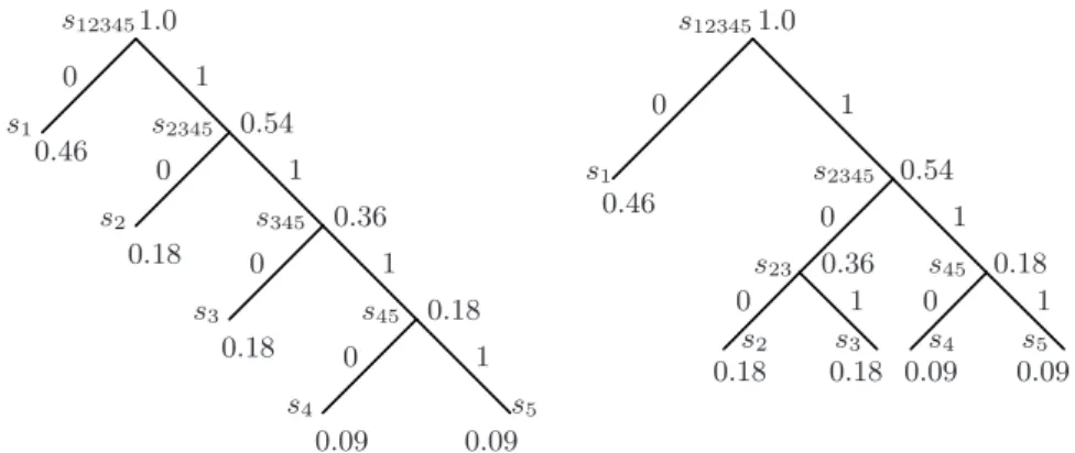
Huffman coding [6] is a widely used and known lossless compression method. It can be found as the only algorithm applied for compression, or as one of many methods used in combination to obtain a more compressed result. One such example is the use of Huffman to compress the result of the transforma-tion done in the joint photographic experts group (JPEG) image compression. The idea behind Huffman is to represent frequently occurring symbols with fewer bits than less frequently occurring symbols. The simplest way to describe the Huffman coding algorithm is by an example. If we consider five symbols s1, s2, s3, s4 and s5 with occurrence probabilities: 0.46, 0.18, 0.18,

0.09 and 0.09. We can build a Huffman tree by merging the two smallest values, these can be chosen arbitrary if more than two values values fits the requirement. This will generate a new node with a value equal to the sum of its child nodes. In our example s4 and s5 are the two smallest values, they

merge into a node with value 0.09 + 0.09 = 0.18. This new node replaces the two smallest values it has merged. The next step in the building process now considers the remaining symbols and the newly created node. There are three instances of the minimum value at this point, we choose the newly created node with value 0.18 and a free node of value 0.18. At this point we have three nodes with the following values 0.36 (the newly created node), 0.18 and 0.46. There are no ambiguities at this point, and the two nodes with smallest values create a node with value 0.54. Then finally the root node is created out of two nodes with values 0.54 and 0.46. The resulting Huffman tree can be seen in Figure 2.1 to the left. Another possible Huffman tree of these probabilities is shown to the right in Figure 2.1. This version is built by selecting the nodes that are not in a subtree when it is possible to choose between free nodes and nodes of a subtree.

Decoding a Huffman encoded stream is also fairly simple, and is also best explained through an example. The method to generate the decoded stream encoded with the Huffman tree seen to the left in Figure 2.1 is as follows: First one simply reads the encoded stream from the beginning and traverses the Huffman tree with the values found in the bitstream, and whenever a leaf node is reached, start at the root again. Let us consider an encoded stream that looks like the following: 0101011011111110, with the first bit to the left. To decode this bitstream, one looks at one bit at a time while traversing the Huffman tree from the root down to the leaves. Which branch to take is given by the value of the bit. When a leaf is reached its symbol is emitted to the output stream. Since the encoded stream can only be interpreted in one way, there is no ambiguity of what symbol to emit.

For the given stream the first two symbols are found as follows: Starting at the root we follow the branch marked with a 0, which leads us directly to a leaf node with symbols1. Then the next bit in the bitstream is considered,

starting at the root node, which leads us to the right, to node s2345. This

is not a leaf node, therefore the next bit in the bitstream is evaluated, and the result is a leaf node, s2, thus this symbol is emitted to the output. If

this is done with the whole bitstream the result is the following output:

s1s2s2s3s5s4. 0 0 0 0 0 0 0 0 1 1 1 1 1 1 1 1 s1 s1 s2 s2 s3 s3 s4 s4 s5 s5 s12345 s12345 s2345 s2345 s345 s45 s45 s23 1.0 1.0 0.46 0.46 0.54 0.54 0.36 0.36 0.18 0.18 0.18 _0.18 0.18 0.18 0.09 0.09 0.09 0.09

Figure 2.1: Two different Huffman trees for the probabilities s1 to s5

2.1.4

Parallel approaches

Huffman decoding and decoding of run-length encoded streams are algo-rithms that are sequential in their nature. While decoding a Huffman com-pressed bit string it is impossible to tell at which position the next symbol will occur without processing the previous bits. There are methods to par-allelize decoding of Huffman bit strings, as will be discussed in Section ??.

2.1. COMPRESSION 9

One simple method that does not scale well is to introduce an offset table before the bit string. This offset table could tell where the different blocks of output data can start their decoding within the encoded bit string. The down side is that this would also require storage and that it does not scale very well for many processing units. One reason is obviously the growth of the lookup table too support a given number of process, and too many entries would give an overhead so great that it would actually result in a growth in the data.

2.1.5

Image compression

The main idea of image compression is the same as for other compression scenarios, exploit the redundancy in the data to make it smaller. There are basically two ways of doing this on images, lossless and lossy. Given that noise to some degree is acceptable in images without perceptible visual artifacts, lossy compression is often used. The lossy compression schemes used on images uses a transformation to compact the information. Gathering the information into a small region due to decorrelation result in possibility to discard data with coefficients close to zero (Salomon [5]). As for lossless compression, it does not introduce any noise, but the compression ratio is not as good as the lossy compression.

The are three major steps in compressing an image with lossy compres-sion:

1. Decorrelation (through a transformation) 2. Quantization

3. Entropy encoding

More details about these steps are given in Section 2.2.

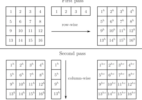
The first step, decorrelation, is achieved through a transformation. If this transformation is separable it can be done in one dimension then in another, and produce the correct result. Separable filters are desirable due to their lower computational complexity. Details around separable filtering are given in Section 2.2.6.

The layout of the three-dimensional (3-D) seismic data is as depicted in Figure 2.2. It consists of two-dimensional (2-D) images stacked upon each other in the depth direction. Image compression for 3-D seismic data is based on the same methods as for 2-D images. Instead of using two passes with a separable filter, one for each dimension, there are three passes. First all the images in the stack are processed as the two dimensional case. Second

height height width width depth depth

Figure 2.2: Arrangement of images in a stack for 3-D seismic data

the filter is applied on all the images in the depth direction. That is as interpreting the values in the depth and height directions as another 2-D image.

Compressing seismic data while considering three dimensions is of great advantage, because of the correlation that exists between the images in dif-ferent directions. An example is the correlation that exists between values in the horizontal direction of seismic images both in depth and in width. As the changes in these directions are small and similar to each other, that is, slow varying.

2.2

Subband coding

The following sections will describe theory related to subband decomposition and coding. Starting out with decimation and interpolation in Section 2.2.2, followed by quantization in Section 2.2.3. Then in Section 2.2.4 and Section 2.2.5 representation of of these stages will be presented.

It can be shown that block transforms are a special case of filter banks that have filter length N, N channels, and a down-sampling by N.

2.2.1

Overview of subband coding

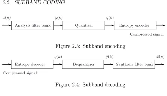
The encoding and decoding processes are presented in Figure 2.3 and 2.4. As can be seen both encoding and decoding is accomplished in three stages. Encoding starts with the analysis transformation, then quantization and fi-nally the entropy encoding. As for the decoding this process is reversed, and the stages are entropy decoding followed by an inverse quantizer and at the final stage synthesis transformation.

2.2. SUBBAND CODING 11 replacemen

Analysis filter bank Quantizer Entropy encoder

Compressed signal

x(n) y(k) q(k)

Figure 2.3: Subband encoding replacemen

Entropy decoder Dequantizer Synthesis filter bank

Compressed signal

q(k) yˆ(k) ˆx(n)

Figure 2.4: Subband decoding

2.2.2

Decimation and interpolation

Decimation and interpolation are operators that processes the samples of a signal. Decimation is the process of reducing the number of samples by an integer factor of M. This results in a reduced sample rate of the same factor. As for the interpolation operator, it does the opposite of the decimation operator, it increases the sampling rate by an integer factor of M. Both of these operations is done after a filter that usually is low-pass. The filter is followed either by a sub sampler, also called down-sample, for decimation, and for interpolation an up-sampler.

The up-sampler inserts zeros between the samples, such thatM−1 zeroes are inserted between the samples. What the down-sampler does is to pick each Mth sample from the original stream, creating a new list of samples indexed 0 for the first sample and 1 for the Mth _{sample taken from the} original stream, and so forth.

As we shall see later, these operators are used in the different stages of the transformation. The down-sampler in the analysis stage, and the up-sampler in the synthesis stage. They are depicted as ↓M for the down-sampler and

↑M for the up-sampler.

2.2.3

Quantization and inverse quantization

There are two well known quantization methods mentioned through out liter-ature, scalar quantization (SQ) and vector quantization (VQ). We will only focus on scalar quantization in this text. SQ is a special case of VQ where the number of dimensions is equal to one. We will use scalar quantization and quantization interchangeably in the rest of the text, unless stated otherwise. Quantization is a process that “ ‘. . . restrict[s] a variable quantity to dis-crete values rather than to a continuous set of values’ ” as described by

Salomon [5] who refers to a dictionary. One way to quantize values is by finding the largest absolute value in the input, then use this when scaling the input data into the integer representation. Mapping into the signed integer range can be done with

$ y(k) max(abs(y(k))) × I 2 % , (2.1)

where I is a constant representing a value that is one greater than the maximal value of the integer representation. As examples of natural choices for the value of the constant I are byte (octet) representation1 _{or word}

representation (here two bytes). This gives I = 28 _{= 256 for bytes and}

I = 216 = 65536 for words.

Equation 2.1 will map the source data into the range of the integer rep-resentation2_{, except at the positive end, where it will be possible to get an}

integer value 1 integer outside the range, as an example 128 is one outside the range of 8-bits signed values. If necessary this will be corrected in the quantization process when the index is calculated, as will soon be explained. This is the stage in the signal compression that introduces the loss of in-formation by using coarser representation of the data values. Therefore it is important to set the quantization to adjust the desired compression ratio and thus the loss.

We use the mid-tread uniform threshold scalar quantizer as described in the PhD thesis of Røsten [2]. The quantizer is actually called a mid-tread uniform threshold scalar quantizer with dead-zone, but for convenience we will just present it as in the previous sentence. This scalar quantization has a dead-zone with a total width T = 2β ×∆ where β > 0, around zero. In the equation for T the ∆ symbol represents the distance between quantizer decision levels, and is known as step-size. The variable β adjusts the size of the dead-zone, and for image compression β = 0.5 is often used, this gives no dead-zone. It is common to use β = 0.6 for compression of seismic data. Compression ratio below 1:10 requires a β < 0.5 to avoid too much quantization noise according to Røsten [2].

i=      I/2 +b(y(k) +T /2)/∆c, y(k)≤ −T /2 I/2, −T /2< y(k)< T /2 I/2 +d(y(k)−T /2)/∆e, y(k)≥T /2 (2.2a)

Equation (2.2a) gives the quantizer indices into the γ function of the quantizer. According to Røsten [2], SQ can be described as a non-linear

1_{An octet is 8 bites in size. The bytes in this text has the same size as an octet.} 2_{Assuming two’s complement.}

2.2. SUBBAND CODING 13

mapping of ym(k) ≡ y(k) ∈ R to a finite set γ ={γ(0), γ(1), . . . , γ(I−1)}. Where the indices i = 0,1, . . . , I − 1 of the γ(i) function are called the quantizer indices and the results of the gamma function is the quantizer levels.

γ(i) = (i−I/2)×∆ (2.2b)

In the subband coding system, quantization and inverse quantization is the stage just after the analysis filter bank and just before the synthesis filter bank, respectively (see Figures 2.3, 2.4 and 2.5). The output of the quantizer is denoted by q(k) and the reconstructed signal by ˆy(k). q(k) can be seen in Figure 2.3 and ˆy(k) in Figure 2.4 (the inverse quantizer is called “dequantizer” in this figure). The quantizer selects the index i according to Equation (2.2a), where I is even. The inverse quantizer finds the quantizer representation level by equation (2.2b). The dynamic range of the quantizer is given by

y(k)<−I/2×∆−T /2 and y(k)>(I/2−1)×∆ +T /2.

and is exceeded if any value is outside. If that happens the value ofi should be replaced with i= 0 andi=I−1 for the given equation, respectively.

2.2.4

Analysis stage

The analysis stage is where the input signal is decomposed into subbands. This results in a decorrelation of the signal as well as concentration of the energy into a minimum number of subbands [2]. After this stage quantization takes place as described above in Section 2.2.3. This introduces compression noise due to an approximation of the samples, since it is assumed that perfect reconstruction is possible. Consequently it is at the quantization stage that loss is introduced to the compressed signal.

Our subband coding scheme is based on the works of Røsten [2] and will now be described. It consists of M-channel parallel-structured uniform filter banks with non-unitary linear-phase near-perfect reconstruction (PR) properties for both analysis and synthesis filters. An illustration of such a system with M-channels can be seen in Figure 2.5. The number of subband filter banks, M, is equal to eight, and the number of taps (denotedL) is 32. If given an one-dimensional (1-D) input by x(n) for n = 0,1, . . . , N −1 the uniform analysis filter bank will produce a decomposition into M subbands with K subband samples in each.

The analysis filter is denoted by hm(l) for m = 0,1, . . . , M −1 and l = 0,1, . . . , L−1 and the subband signals by ym(k) for k ∈ N. The function

for reconstructed signals is denoted by ˆym(k). For the synthesis filter the function is given by gm(l). The filters for analysis and synthesis is given by the following equations (which can be found in Røsten [2], and Ramstad et al. [7]) ym(k) = ∞ X n=−∞ hm(kM −n)x(n) (2.3a) and ˆ x(n) = M−1 X m=0 ∞ X k=−∞ gm(n−kM)ˆym(k), (2.3b) respectively.

For 2-D and 3-D subband decomposition and reconstruction separate fil-tering in each dimension is performed. For the 2-D case this can be done by first filtering row-wise then column-wise, or the other way around, at the analysis stage, and for the synthesis stage the ordering of filtering is re-versed. The 3-D case is similar to the 2-D case just with an expansion of one more dimension, see Section 2.1.5. For details concerning separable filters see Section 2.2.6.

When doing subband decomposition, expansion of the signal is prevented by adhering to three constraints. Firstly, the length of the input signal, N, divided byM must give K whereK is the number of samples in a subband, ideally this should be equal for all the subbands. Secondly, extension of the input signal at the edges has to be considered. Thirdly, the subband samples has to be critically down-sampled by M. The result of following these constraints is a reconstructed signal ˆx(n) that has the same length as the original x(n). Furthermore, it gives a maximally decimated filter bank system that has the property K ×M = N. More details of the second constraint is given in Section 2.2.7.

2.2.5

Synthesis stage

In this stage signals are reconstructed from subbands into the original signal, if the signal from the analysis stage is used without modification near-PR is achieved. Loss of precision is mainly due to the quantization that introduces noise, as mentioned earlier.

Otherwise the synthesis stage is basically equal to the analysis stage, except for different filter and transformation function. The equation for the synthesis filter banks is given in Equation 2.3b.

2.2. SUBBAND CODING 15 x(n) ˆ x(n) ↓M ↓M ↓M ↑M ↑M ↑M Σ Σ h0(l) g0(l) y0(k) yˆ0(k) h1(l) g1(l) y1(k) yˆ1(k) hM−1(l) gM−1(l) yM−1(k) yˆM−1(k)

Analysis filter bank Synthesis filter bank

B

la

ck

b

ox

Figure 2.5: Figure adapted from Fig. 1.10 and Fig. 2.5 in [2]. Overview of a M-channel maximally decimated filter bank system with a black box in the middle.

2.2.6

Separable filters

Applying filter transformation to a 2-D image can be done in two ways, as a convolving mask or as two separate transformations one in the horizontal direction followed by one in the vertical direction, or vice versa. This last method works on filters that are separable and has great benefits with respect to amount of calculations performed. Let us consider the Sobel operator as described by Gonzalez and Woods [8]. The filter mask of the Sobel operator with size 3×3 is as shown in Table 2.1.

Table 2.1: Sobel operator of size 3×3.

-1 0 1

-2 0 2

-1 0 1

If we use the method of spatial filtering, described by Gonzalez and Woods [8], of an image of size M ×N and a mask of size m×n. The transformed image is given by,

g(x, y) = a X s=−a b X t=−b w(s, t)f(x+s, y+t) (2.4) where,a= (m−1)/2 andb= (n−1)/2. Equation 2.4 has to be applied for

all the values ofxandyin the image, that is forx= 0,1, . . . , M−2, M−1 and

y= 0,1, . . . , N −2, N−1. As can be seen the number of multiplications for each element ism×n. This filter mask can also be written as a combination of two vectors multiplied together. If denoted as v for vertical and h for horizontal they may be represented as,

v =    1 2 1    h= [−1 0 1] (2.5)

This equation shows how a separable 2-D filter can be decomposed into two vectors. Now, it is possible to transform an input image with the Sobel operator by first doing a vertical transformation then a horizontal transfor-mation. Doing the transformation this way results in m+n multiplications per transformed element. Thus, it is easy to see that the amount of calcula-tions needed to do the transformation is drastically reduced with separable filters. The amount of calculation to filter an image without using separable filters isM N mn versus M N m+M N n =M N(m+n) for separable filters.

A figure illustrating the process of doing filtering in two separate steps, first horizontal then vertical is seen in Figure 2.6.

1 1 2 3 4 2 3 4 5 6 7 8 9 10 11 12 13 14 15 16 1h 1h 1h 2h 2h 3h 3h 4h 4h 5h 5h 5h 6h 6h 7h 7h 8h 8h 9h 9h 9h 10h 10h 11h 11h 12h 12h 13h 13h 13h 14h 14h 15h 15h 16h 16h 1hv ₂hv ₃hv ₄hv 5hv 6hv 7hv 8hv 9hv 10hv 11hv ₁₂hv 13hv₁₄hv ₁₅hv ₁₆hv First pass Second pass row-wise column-wise

2.2. SUBBAND CODING 17

2.2.7

Filter extension

To preserve the perfect reconstruction (PR) property of a signal in an analysis-synthesis filter bank, care has to be taken at the boundaries of a signal. This is due to the the overlapping of unit pulse responses of both the analysis and synthesis filter channels. The reason is that signal segments are reconstructed with an added influence from adjacent signal parts [7].

The solution is extension of the signal, according to Ramstad et al. [7], there are only two known methods of extending the finite length input signal while still preserving the PR property. This without generating additional information to be sent along with the signal. The methods are known as, circular extension and mirror extension.

Circular extension is achieved through repeating the finite input signal at its extremities. Given an input signal with a length of K samples, its extended signal will have a periodicity of K. As pointed out by Ramstad, et al. [7] it can be proved that the periodic property of an input signal is preserved after time-invariant linear filtering. Thus, each channel signal have a period ofK before decimation. The period after after decimation is given by

K =pN, (2.6)

where N is the decimation factor and p is the period for each of the sub-band signals. Furthermore, given that the decoder has to know each infinite subband signal for perfect reconstruction, which is fulfilled through the peri-odicity pof each subband, it is thus sufficient to transmitp samples for each subband [7].

Finally, we take at look at the mirror extension method. This method is similar to that of circular extension with a little twist, the signal is first mirror reflected at one endpoint, then periodic extensions are performed at the signal that now has double length. The benefits of mirror extension compared to circular extension is the avoidance of discontinuities present in circular extension [7].

Instead of taking advantage of periodicity, the mirror extension preserves the symmetry on both sides of the mirror points. As stated by Ramstad et al. [7], if a linear phase filter is applied to a symmetric signalx(n) the output is symmetric. In general if an input signal have the same symmetry as the filter, symmetric or not, the result is symmetric, and if they differ the result is anti-symmetric. This same relation is valid for whole-sample symmetry and half-sample symmetry. Half-sample symmetry is the case when the symmetry is between two samples contrary to whole-samples where the symmetry is at a sample.

an even-length symmetric filter, h. Assume that the filter has half-sample symmetry and a length of four. Extension of the input signal can be done with either whole- or half-sample symmetry. Since we want an output that has whole-sample symmetry we should exploit the facts mentioned in the previous paragraph. Thus, we do a half-sample expansion of the input signal, giving us two half-sample sources which results in a whole-sample output. An illustration showing how this might look, is given in figure 2.7. The figure illustrates the extended input and the result before any decimation is performed.

Figure 2.7: At the top the extended input, and at the bottom the filtered output.

The filtered signal now has 17 distinct values. Since the critical decima-tion with factor N result in a transfer of 16/N out of the 17 samples, care has to be taken while choosing the samples. Ramstad et al. [7], gives two criteria that has to be fulfilled: First, avoid picking whole-sample symmetry samples, that is -1 and 17. Second, it is important that the samples on the opposite side of the symmetry points have the correct distance. If the correct samples are chosen they have the same value at both sides.

2.2.8

The “black box” stage

Within the “black box” two sub-stages takes place, quantization (Section 2.2.3) and entropy coding. The entropy coding is to reduce the data amount

2.2. SUBBAND CODING 19

used to represent the information. It may be a single method such as Huff-man coding, arithmetic coding or simply RLE, or a combination of several compression methods. The entropy encoding and decoding takes place after the quantization, and before the inverse quantization, respectively. Details about these compression methods was given in Section 2.1 and quantization was presented in Section 2.2.3.

Chapter 3

GPU programming

Since the the topic is decompression of seismic data on GPUs we will look at the architecture of modern GPUs, focusing on the NVIDIA Tesla archi-tecture. Given that the application of interest is not designed with a CPU in mind, description of the CPU architecture is not described here. Section 3.1 and 3.2 and its subsections is taken from an earlier work of mine [9], and contains minor changes.

3.1

NVIDIA’s Tesla architecture

To get a better understanding of how the GPU works, a presentation of the NVIDIA Tesla architecture will be given, based on [10] and [11].

Within Tesla based GPUs you will find groupings of texture/processor clusters (TPCs). Within a TPC you will find 2 streaming multiprocessors (SMs). Further, inside a SM there are 8 streaming-processors (SPs) cores. An overview figure of this architecture can be seen in Figure 3.1, and more detailed figures of the TPC (Figure 3.2) and SM (Figure 3.3). At the highest abstraction level we find the streaming processor array (SPA), which contains all from one TPC and up wards. As an example the NVIDIA QuadroFX 5800 has 240 SPs and 30 SMs.

The TPC contains the following elements: a geometry controller, a streaming multiprocessor controller (SMC), two streaming multiprocessors (SMs), and a texture unit (see Figure 3.2). The most interesting parts within a TPC for us is the SMs. Inside the SM you will find an instruction cache, a mul-tithreaded instruction fetch and issue unit (MT issue), a read-only constant cache, 8 SP cores, 2 special-function units (SFUs), and a 16 kilobytes of read/write shared memory, shown in Figure 3.3).

A SP core contains a scalar multiply-add (MAD) unit, resulting in eight 21

MAD units for a SM. For transcendental functions and attribute interpo-lation the SFU is used. Each SFU contains four floating-point multipliers. The texture unit can be used as a third execution unit by the SM within the TPC. The SMC and raster operation processor (ROP) units implement ex-ternal memory load, store as well as atomic access. Between the SPs and the shared-memory banks there is a low-latency interconnect network providing shared-memory access.

The SM is hardware multithreaded to be able to execute several hundreds of threads in parallel while running several programs. The number of threads that can be executed concurrently in hardware with zero overhead for a SM, varies from 768 to 1024 with compute capability 1.0 and 1.2 respectively [11].

3.1. NVIDIA’S TESLA ARCHITECTURE 23

The SM in the Tesla architecture uses what NVIDIA calls single-instruction, multiple-thread (SIMT). The SM’s SIMT multi-threaded instruction unit’s responsibility is creating, managing, scheduling and executing threads. Threads are executed in groups of 32 parallel threads known as warps. Creation of threads is lightweight, as is fast barrier synchronization between threads, which can be issued with an instruction. This gives a very efficient and fine-grained parallelism. Each SM manages a pool of 24 warps, with a total of 768 threads, or 32 warps with a total of 1024 threads for compute capability 1.2 or higher, an example is GeForce GTX 280 [11], we will assume 24 warps in a pool for the rest of the document, unless stated otherwise. The SM selects one of the warps, in the pool of 24, to execute a SIMT warp instruction, each cycle. A warp instruction issued is executed as two sets of 16 threads over a period of four processor cycles. It should be noted that the SP cores and the SFU units executes instructions independently, so by issuing instructions between them on alternate cycles, it is possible for the scheduler to keep both working. The choice of warp is based on a scoreboard that qualifies each warp every cycle. Warps that are ready is prioritized by the instruction scheduler, it then select the one with highest priority for issue. Prioritizing is based on warp type, instruction type, and “fairness” to executing warps within the SM.

Memory instructions provided by the Tesla architecture are of the type load/store. These instructions use integer byte addressing and registers with offsets through address arithmetic. There are three kinds of memory spaces accessible through these load/store instructions: local memory, shared mem-ory and global memmem-ory. The properties of the different memmem-ory spaces gives varying performance, care has to be taken to utilize the correct memory space for optimal performance. We will consider this aspect in greater detail later, when we look at coalesced memory access. Each of the memory spaces have their own instructions for load and store, they are load-global, store-global, load-shared, store-shared and load-local, store-local. Memory bandwidth is improved by coalescing load/store instructions when accessing global and local memory.

3.2

NVIDIA CUDA

NVIDIA compute unified device architecture (CUDA) was introduced by NVIDIA to allow programmers access to the graphics hardware without go-ing through a graphics application programmgo-ing interface (API), such as OpenGL or DirectX. It is a programming model that extends the C program-ming language through the use of special declarations and an API. The

ap-3.2. NVIDIA CUDA 25

Figure 3.3: Figure of the SM from [10]

plication is built on top of a NVIDIA CUDA driver that communicates with the targeted device. Over this driver there are abstractions, such as NVIDIA CUDA runtime and NVIDIA CUDA libraries. NVIDIA CUDA runtime is an abstraction that simplifies the programming as is the NVIDIA CUDA libraries. The libraries include CUFFT and CUBLAS, that implements fast Fourier transform (FFT) and basic linear algebra subprograms (BLAS) re-spectively.

3.2.1

NVIDIA CUDA extensions to the C

program-ming language

Programming C for CUDA provides some extension to the C language:

• Function type qualifiers

• Variable type qualifiers

• Built-in variables

Function type qualifiers specify if a function executes on the host, or on the device. It also specifies if it is callable from the host or the device. The qualifiers are device , global and host . Functions having

device qualifier is only callable from the device, and executes on a device. In contrast to those having global , they are callable only from the host, but executes on the device. Finally, the code that are handled only by the host have host as a qualifier, or simply no qualifier. It is possible to combine host with device , in which case code for both host and device is compiled.

Variable type qualifiers specify where a variable is to reside in memory. They are device , constant and shared . For variable type qual-ifiers as with function qualqual-ifiers the device specifies that the variable shall reside on the device. In addition to this qualifier it is possible to specify which memory space on the device, being either constant or shared . The execution configuration specifies how the kernel is executed on the device from the host. It is specified by the use of

¡¡¡DimGrid, DimBlock, NumSharedMem, Stream¿¿¿

Both DimGrid and DimBlock are of type dim3, it has three members: x, y and z. NumSharedMem is of type size t and Stream of type cudaStream t. DimGrid specifies the dimension of the grid, that is the number of blocks. DimBlockspecifies the dimension of each block in the grid, that is the num-ber of threads per block. NumSharedMem specifies the number of bytes in shared memory that is dynamically allocated. Finally, Stream specifies the associated stream, default is 0. An example of calling a function is given in listing 3.1.

The built in variables are the following:

• gridDimof type dim3, holds the dimensions of the grid.

• blockIdx of type uint3, a vector type with the components accessed through x, y and z as with dim3. It has the block index within the grid while running a kernel.

• blockDimis of dim3and holds the dimensions of a block, and thus the number of threads.

• threadIdx of typeuint3 contains the thread index within a block.

• warpSize is an int type containing the size of the warp in number of threads.

3.2. NVIDIA CUDA 27

Listing 3.1: Calling a NVIDIA CUDA kernel g l o b a l void f o o (f l o a t ∗a r g ) ; // p r o t o t y p e o f f o o

f o o<<<DimGrid , DimBlock , NumSharedMem , Stream>>>(a r g ) ;

These built-in variables cannot be assign values, and it is not allowed to take the address of them.

3.2.2

NVIDIA CUDA’s memory hierarchy

Knowing the memory hierarchy is of great importance to able to write ef-ficient code with NVIDIA CUDA. Since there are no cache on the local memory or global memory, accessing these gives a penalty between 400 and 600 clock cycles of memory latency.

The hierarchy is as follows [11]. Each thread has a per-thread local mem-ory, each block contains a shared memory seen by all threads in the block, having a lifetime as long as the block. Then there is global memory acces-sible by all threads. In addition to these, there are special type of memory, known as texture and constant memory, both are actually constant. All of the mentioned memory spaces are optimized for different purposes. Texture memory for instance, offers different addressing modes, and it also has data filtering support for some specific data formats.

To maximize memory bandwidth, it is crucial to access the underlying memory hierarchy in the correct manner. If possible, for global memory what is called coalesced memory access should be used. Shared memory access should be done without bank conflicts to avoid reduced bandwidth [11]. Details around how this is done follows in the subsequent sections.

3.2.3

Shared memory

Because of the limited number of registers, 8192 for devices with compute capability below 1.2 and 16384 for devices supporting 1.2. This is the number of registers for each multiprocessor, in addition to this there are 16 kilobytes of shared memory for each multiprocessor. This memory is organized into 16 banks for devices of compute capability 1.x. Accessing different banks can be done simultaneously, therefore accessing n different addresses falling into

ndifferent banks yields bandwidth that isn times that of one single memory module (bank).

If bank conflicts occur, those addresses that map to same bank are serial-ized. This is done by the hardware, and results in as many separate conflict-free requests as necessary. The number of separate memory requests, if there

are n of them, is called a n-way bank conflict. Consecutive 32-bit words in shared memory goes into subsequent banks, and each bank has a bandwidth of 32-bits per two clock cycles.

Further, devices having compute capability 1.x have warp size of 32, and the bank count is 16. When a warp issues a memory request for shared memory, is it split into two request, one for each half-warp. Handling the first half-warp then the second, thus there are no bank conflicts between threads in the two half-warps.

3.2.4

Global memory

Due to the importance of utilizing the memory when doing high performance computation on GPUs, the coalescing of memory access will be described [11]. There are differences of the first NVIDIA CUDA capable devices and the new ones, classified by what is called compute capability. Devices with compute capability 1.0 and 1.1 are more restricted than that of 1.2 or higher when it comes to coalesced memory access.

The implementation was written with the strictest of the coalesced mem-ory access patterns in mind, such that devices with compute capability below 1.2 and those compatible with 1.2 should be able to make use of coalesced memory access. Even if the kernels was designed to follow the strictest pat-tern as best as possible, both the access patpat-terns are presented, that is for devices below and those including and above 1.2. The latter to show how it eases the way to get coalesced memory access on newer devices.

Now, coalesced memory access is presented based on NVIDIA’s CUDA programming guide [11]. Coalesced memory access makes what could be several single memory transactions into one single memory transaction. First, devices with compute capability below 1.2 is described, followed by those including and above 1.2.

Compute capability below 1.2 Three conditions have to be satisfied for global memory access to be coalesced into one or two accesses. Coalescing is valid for all the threads within a half-warp if the following three conditions is fulfilled.

It is a requirement that the threads access either, 32-bit, 64-bit or 128-bit words. The latter case gives two memory transactions each of 128 bytes. Further all the 16 words that are accessed has to lie in the same segment or twice size for the 128-bit case. According to the programming guide for NVIDIA CUDA [11], the global memory is partitioned into segments that are of size 32, 64 or 128 bytes, and aligned to those sizes. The third condition

3.2. NVIDIA CUDA 29

that has to be satisfied is that the threads accesses the words in sequence. Which means that the ith thread in a half-warp has to access the ith word. If not all of the above conditions is satisfied, a memory access is issued for each of the threads. Accessing words of greater sizes reduces the bandwidth, for example accessing 64-bit words gives reduced bandwidth compared to 32-bit words, and so on. Figure 3.4 shows a coalesced memory access on the left side, and the right side shows a non-coalesced memory access.

Compute capability 1.2 and above Now, that the coalesced memory access conditions for compute capability 1.2 and below has been described, it is in place do describe that of compute capability 1.2 and above.

Coalesced memory access to global memory occurs for a half-warp when-ever the words accessed by all the threads lie in the same segment. The segment has to be of size 32 bytes, 64 bytes and 128 bytes, for accesses to respectively 8-bit, 16-bit and for the last case 32-bit or 64-bit words, it is assumed that each thread accesses the the same word size.

The access pattern for addresses requested for a half-warp is not re-stricted, it is even possible for multiple threads to access the same address. Clearly this is not as strict as for devices of lower compute capabilities. An example of this can be given as follows: A half-warp addresses words in n

different segments, this results in n memory transactions for devices of com-pute capabilities above 1.2. Now, devices with comcom-pute capabilities below that, issues 16 different transactions, which occurs as soon asn is above 1.

Even if not all words in a segment is used, all words are read. To reduce the waste of memory bandwidth, the smallest segment that contains the requested words is chosen. So if all the words lie in one half of a segment, and there exists a segment half of the original, the smaller one is chosen for transaction. Figure 3.5 shows different scenarios for devices of compute capabilities above 1.2.

Figure 3.4: Coalesced memory access versus non-coalesced memory access for devices with compute capability 1.0 and 1.1, [11].

3.2. NVIDIA CUDA 31

Figure 3.5: Coalesced memory access patterns for compute capability above 1.2

Chapter 4

Methodology

This chapter describes details concerning the implementation of different parts of the system. Starting with RLE in Section 4.1, then subband trans-formations in 4.2. Furthermore in Section 4.3 the Huffman implementation details are presented. Then the transpose functions are presented in Section 4.4.

4.1

Run-length encoding implementation

In this section we will present the GPU implementation of RLE decoding. It is a fairly straight forward implementation of RLE with minor modifications to speed it up on GPUs.

4.1.1

Layout of the RLE data

The format of the RLE is as described in Section 2.1.2. That is, a counter followed by a single value or a number of different values. The implemented RLE encoder uses a 32-bit type. The counter either gives the number of times to repeat a value or the number of following bytes that should be copied to the output stream. This is marked by the counter by having a positive value if the next byte is to be repeated, and a negative value if the following bytes are to be copied directly to the output, the absolute value gives the actual count.

Furthermore the modification done to the RLE-decoding on the GPU is the addition of a table with offsets into the input stream where the decoding can start. The motivation for this offset table is mainly to increase per-formance. A run-length encoded stream has to be decoded from the start because there are no way of telling where a counter starts without following

the counters from the start of the input.

To distribute the workload of decoding a RLE encoded stream among several processors the encoded stream is partitioned into smaller sections. This allows the different processors to work on their section of the encoded stream and produce their own output section. The decomposition of an encoded stream is such that the sections produced by each processors are about the same size. This is achieved by choosing the counters that are close to the given positions in the original stream. If we have a table with two offsets, we would start at the beginning of the encoded input stream and at a position in the encoded stream that would start writing close to the middle of the decoded output stream.

The offset table contains three variables for each entry: input position,

output positionand atag count. The input position gives the offset in number of bytes from the beginning of the encoded stream. The output position gives the offset in number of bytes from the beginning of the decoded stream. Finally, tag count gives the number of the tag from the beginning of the encoded stream. This last variable is used to keep track of the extent of the section being decoded, by knowing the tag count of the next section, decoding can proceed until the tag count of the section being decoded equals the tag count of the next section. A pseudocode of the RLE-decoding can be seen in Algorithm 4.1.1.

4.1.2

The RLE decoding kernel

Instead of using branches to select which section of the encoded stream a group of threads should handle, the thread number is used to select the correct section. The kernel is designed to handle a RLE-stream that is divided into eight parts. To be able to fully utilize coalesced memory accesses it has 128 threads assigned to it. This way each section has 16 threads available to utilize coalesced memory access while reading or writing to global memory.

The partitioning is as follows: First, the thread ID is shifted to the right such that the three most significant bits of the maximum number of threads in a block, here 128, can be found as the three least significant bits. Then a mask is used to ensure that the only valid values are in the range 0 to 7. The result is that thread IDs in the range 0–15 belong to section 0, thread IDs in range 16–31 in section 1 and so on. An illustration of this scheme is given in Figure 4.1. Figure 4.1 illustrates how the binary number with range 0002 to 1112 maps to the different sections in the decoded stream1.

1_{We denote the radix by subscript, e.g. 11}

2is 3 (decimal) in radix 2, and assume radix 10 as the natural radix (decimal).

4.1. RUN-LENGTH ENCODING IMPLEMENTATION 35

Algorithm 4.1.1: _rle-decode(input, output, lenOut, threadID)

local currentP os, posOut, startT ag, stopT ag, currentT ag

(currentP os, posOut)←_GetPositions(input, threadID) (startT ag, stopT ag)←_{GetTagNumbers}(threadID)

repeat

comment:Read counter from input stream.

count←_getCount(input[currentP os])

if count≥0 then          symbol ←_{getNextSymbol}() for i←1to count do (

write(output[posOut], symbol)

posOut←posOut+ 1

else

 



comment:Copy countsymbols from input to output.

copy(output[posOut], input[currentP os],abs(count))

currentP os←currentP os+_abs(count)

currentT ag ←currentT ag+ 1

Starting with the initial length at the top, where binary numbers starting with a zero as the leftmost digit handles the first part of the output stream. Furthermore binary numbers starting with 00 handle the first quarter of the output stream. At the bottom of the figure, section 0 to 1 and section 1 to 2 are handled by binary numbers 000 and 001.

Initial length

0xx 00x

0 1 2 3 4 5 6 7 8

Figure 4.1: Illustration of division based on a binary number

4.2

Subband transform implementation

The kernel of the implementation doing the most compute intensive task, subband transformation, is presented in this section. There will be given a thorough description of how it was designed to gain the performance it has. First the serial implementation of the synthesis stage in the subband coding (CPU) is briefly described, then the conversion to a parallel version is given (GPU).

4.2.1

Description of the implementation

First, the serial implementation is described to give a natural transition for the parallel implementation, and because the serial version maps closer to Equation 2.3b than the parallel version.

A pseudocode of the serial version is given in Algorithm 4.2.1, this algo-rithm gives an overview of the synthesis stage. Pseudocode for the upSample-AndFilterfunction is given in Algorithm 4.2.2 The coefficients used is given in Appendix A, the algorithms presented use the coefficients for synthesis which can be see in Table A.2 and A.4.

The 1-D subband synthesis algorithm starts by padding (mirroring) the input signal at both ends, that is, at the start and at the end. The procedure