Performance Modeling of Softwarized Network
Services Based on Queuing Theory with
Experimental Validation
Jonathan Prados-Garzon, Pablo Ameigeiras, Juan J. Ramos-Munoz, Jorge Navarro-Ortiz, Pilar Andres-Maldonado,
and Juan M. Lopez-Soler
Abstract—Network Functions Virtualization facilitates the au-tomation of the scaling of softwarized network services (SNSs). However, the realization of such a scenario requires a way to determine the needed amount of resources so that the SNSs per-formance requisites are met for a given workload. This problem is known as resource dimensioning, and it can be efficiently tackled by performance modeling. In this vein, this paper describes an analytical model based on an open queuing network of G/G/m queues to evaluate the response time of SNSs. We validate our model experimentally for a virtualized Mobility Management Entity (vMME) with a three-tiered architecture running on a testbed that resembles a typical data center virtualization environment. We detail the description of our experimental setup and procedures. We solve our resulting queueing network by using the Queueing Networks Analyzer (QNA), Jackson’s networks, and Mean Value Analysis methodologies, and compare them in terms of estimation error. Results show that, for medium and high workloads, the QNA method achieves less than half of error compared to the standard techniques. For low workloads, the three methods produce an error lower than 10%. Finally, we show the usefulness of the model for performing the dynamic provisioning of the vMME experimentally.
Network Softwarization, NFV, performance modeling, queuing theory, queuing model, softwairzed network services, resource dimensioning, dynamic resource provisioning.
I. INTRODUCTION A. Contextualization and Motivation
At present, Network Softwarization (NS) is radically trans-forming the network concept, and its adoption constitutes one of the most critical technical challenges for the networking community. Network Functions Virtualization (NFV) is one of the main enablers of the NS paradigm. The NFV concept decouples network functions from proprietary hardware, en-abling them to run as software components, which are called Virtual Network Functions (VNFs), on commodity servers.
Considering the ETSI NFV architectural framework [1], a VNF may consist of one or several Virtual Network Function Components (VNFCs), each implemented in software and performing a well-defined part of the VNF functionality. In turn, a VNFC might have several instances, each hosted in a
Jonathan Prados-Garzon, Pablo Ameigeiras, Juan J. Ramos-Munoz, Jorge Navarro-Ortiz, Pilar Andres-Maldonado, and Juan M. Lopez-Soler are with the Research Centre for Information and Communications Technologies of the University of Granada (CITIC-UGR); and the Department of Signal Theory, Telematics and Communications of the University of Granada, Granada, 18071 Spain (e-mail: [email protected]; [email protected]; [email protected]; [email protected]; [email protected]; [email protected])
single virtualization container like a Virtual Machine (VM). Here we will consider a Softwarized Network Service (SNS) as an arbitrary composition of VNFs. In an SNS, packets enter through an external interface, follow a path across the VNFs, and finally leave through another external interface.
One of the most exciting aspects of the adoption of the NS concept is that it enables the automation of the management operations and orchestration of the future networks [2], thus reducing the Operating Expenditures (OPEXs) of the network. Such management operations include to automatically deploy (e.g., SNSs planning) [3] and scale on-demand (e.g., Dynamic Resource Provisioning (DRP)) [4]–[7] network services to cope with the workload fluctuations while guaranteeing the performance requirements. It involves increasing and reducing resources allocated to the services as needed. However, to realize such a scenario, it is required to determine the required amount of computational resources so that the service meets the performance requisites for a given workload. This problem is known as resource dimensioning, and performance modeling can tackle it efficiently. That is using performance models to estimate the performance metrics of the SNSs in advance and reverse them to decide how much to provision.
Besides the resource dimensioning, the performance models have the following exciting applications in the NS context:
• Network embedding (i.e., how to map VNFC instances to physical infrastructures), in which the system must verify whether some given computational resources assignment will cater to the particular Service-Level Agreement (SLA) end-user demands. The authors in [8] illustrate this QT application.
• Request policing which allows the system to decline ex-cess requests during temporary overloads. The probability of discarding an incoming packet at the edge network elements might be determined by using performance models from the monitored workload and the number of resources currently allocated to the system.
B. Objective and Proposal Overview
The objective of this work is to investigate the application of Queueing Theory (QT) to predict the SNS performance. More specifically, we aim at proposing a QT model of closed-form expressions that predicts the mean end-to-end (E2E) delay suffered by packets as they traverse the SNS. Some works in the literature also propose analytical models to estimate
the performance metrics or carry out resource dimensioning in NFV and multi-tier Internet services (see a related work summary in Section II). Some of these works are also based on QT and have shown its usefulness for the dimensioning problem. However, they lack an experimental validation, which is of utmost importance as otherwise, the validity of the proposed model is questionable. Some other works are based on experimental measurements, but they either do not focus on NFV, or they model a single VNF instead of a composition of VNFs. In this paper, we cover this gap. To the best of our knowledge, this is the first work that experimentally validates a QT-based model that predicts the mean E2E delay of an SNS.
Given the plethora of SNS services with different SLA requirements, different types of VNFs and VNFCs with dis-tinct resource limitations (central processing unit (CPU), I/O, bandwidth), heterogeneous physical hardware underlying the provisioned VMs, and the sharing of common resources in data centers, proposing a model for all possible conditions is a vast task. For this reason, we concentrate on SNSs whose constituent VNFCs execute CPU-intensive applications for packet processing (e.g., virtualized Evolved Packet Core (vEPC), Internet Multimedia Subsystem (IMS), and SGi Local Area Network (SGi-LAN) processing chains like video opti-mizers.). We also assume that VMs do not suffer significant dynamic changes in performance at runtime (DCR) due to resource sharing in the data center [9] (space-shared policy [10]). Moreover, for simplicity reasons, we will further assume that the VNFCs do not apply Quality of Service (QoS) prioritization in the packet processing.
In this work, we use an open network of G/G/m queuing nodes to capture the behavior of the SNSs and estimate their mean E2E delay. Particularly, each VNFC instance is modeled by a queuing node of the queuing network. If the VNF consists of a single VNFC, then the VNF instance is also modeled by a queuing node. The model allows several instances of a given VNFC running in parallel and being hosted in isolated virtualization containers. Additionally, the model considers that different packet flows may follow different routes across the instances of the VNFCs. The model also permits that different virtualization containers (e.g., VM) might offer dis-tinct computing performance, even if they host instances of the same VNFC. The different queues might be attended by multiple servers, each of which stands for a CPU core allocated to the corresponding VNFC instance. Please note that here, the term server is QT jargon, not referring to a Physical Machine (PM).
The resulting network of queues, which models the SNS, is solved by using the technique proposed by Whitt in [11] for the Queuing Network Analyzer, from now on referred to as the QNA method. It is an approximate method to derive the performance metrics of a network of G/G/m queues. It assumes that the queues are stochastically independent even though, they might not be. As a result, the mean E2E delay of an SNS can be estimated by a set of closed-form expressions. This has the benefit that its execution time is meager. Despite that, as we will later show, it provides quite accurate results.
C. Contributions
This article introduces a QT-based performance model for SNSs. The model is targeted at SNSs whose components run CPU-intensive tasks under a space-shared resource allocation policy [10]. The model consists of an open network of G/G/m queues, which is solved using the QNA method [11]. In this way, we can estimate the E2E mean response time of an SNS. The main application of the model is the sizing of the computational capacity to be allocated to a given SNS. Expressly, the model permits to jointly perform the dimensioning of the number of CPU cores to be allocated to each constituent VNFC of the SNS from an E2E delay budget. The main contribution of this paper compared to the existing related literature is the experimental validation of the proposed model. To that end, we consider a Long-Term Evolution (LTE) virtualized Mobility Management Entity (vMME) with a three-tier design (i.e., it is decomposed into three VNFCs) which is inspired by web services. The operation considered for our vMME is similar to that one described in [12]. We developed the three-tiered vMME and deployed it on a virtualized envi-ronment with a substrate hardware infrastructure that emulates a data center. Both the PMs and the virtualization layer were configured to operate under a space-shared resource allocation policy. Besides, we developed a traffic source and a network emulator. The traffic source generates LTE signaling workload according to the compound traffic model described in [13]. The network emulator emulates the inter LTE entities latency, and the control plane functionality of the Serving Gateway (S-GW) and eNodeB (eNB) by answering the request control messages generated by the vMME.
An initial version of the performance model proposed in this paper was described in our previous work [14]. After, it has been applied to the planning and DRP for specific scenarios in [3] and [6], [7], respectively. All those previous works have reported satisfactory simulation results on the accuracy and usefulness of the model. In contrast to our previous work, this article includes the following novelties:
• Enhancement of the generality and accuracy of the per-formance model by considering the impact of the Virtual Links (VLs) on the SNS response time.
• Experimental validation of the performance model for a real SNS deployed on top of the virtualization layer of a micro cloud. Moreover, we extend the validation study by assessing the estimation error of the QNA method for predicting the second-order moments of the internal arrival processes.
• Experimental validation of the model for DRP. We show-case the usefulness of our model in a real scenario for the resource dimensioning and request policing.
Finally, we compare the QNA method with the standard methodologies for analyzing queuing networks (e.g., Jackon’s approach and Mean Value Analysis (MVA)). For example, the methodology for solving Jackson’s networks assumes that arrival and service processes are Poissonian to solve the open network of queues. Results show that for medium and high workloads, QNA method achieves less than half of error
compared to the standard approaches. For low workloads, the three methods produce an error lower than 10%.
The remainder of the paper is organized as follows: Section II provides some background on performance modeling based on queuing networks and briefly describes the related works. Section III describes the system model. In Section IV, we detail the queuing model for SNSs and the QNA method. In Section V, we particularize the model to a specific three-tier vMME use case. Section VI explains experimental procedures, including the description of the experimental setup, the pa-rameter estimation, and the conducted experiments. Section VII provides experimental results for model validation and includes a subsection for measured input parameters of the model. Finally, Section VIII summarizes the conclusions.
II. BACKGROUNDANDRELATEDWORKS
This section provides some background on queuing net-works and briefly reviews models proposed in the literature to assess the performance of softwarized networks. This review also includes some models for multi-tier Internet applications.
A. Queuing Networks
Queueing Networks (QNs) are models that consist of multi-ple queuing nodes, each with one or several servers [15], [16]. In these models, jobs arrive at any node of the QN to be served. Once a job is served at a node, it might either move to another node or leave the QN. The arrival and service processes at any node are typically described as stochastic processes. QNs resemble the operation of communication networks and are thus suitable models to estimate its performance.
In contrast to the performance analysis considering each element in isolation, QNs capture the behavior of the whole system holistically. Then, in the context of softwarized net-works, a QN-based performance modeling approach brings attractive benefits such as:
i) The performance of the whole system can be estimated from the characteristics of external arrival processes. Then it is only required to monitor incoming packet flows to the edge network elements, thus avoiding to install monitors at each network element and saving computational resources for monitoring purposes [17]. ii) The resource dimensioning of the different VNFCs of an
SNS, which is a fundamental part of the proactive DRP, can be performed at once from the overall performance targets. For instance, given an overall delay budget of the system, it is possible to define algorithms that rely on QN models to optimally distribute the delay budget among the different VNFCs. This approach leads to resources saving, as shown in [6].
Given the present state of the art, only those QNs that admit a product-form solution, i. e., the joint probability of the QN states is a product of the probabilities of the states in individual queuing nodes, can be analyzed precisely [15], [16]. Specifically, mainly BCMP (Baskett-Chandy-Muntz-Palacios) networks [18] have a product-form solution. There are three primary methodologies to solve exactly a network with a product-form solution: i) Jackson’s network methodology, ii)
MVA, and iii) the convolution algorithm (for more information on these methods, please refer to [15], [16]).
However, few real network systems meet the conditions of BCMP networks (see [18]) and admit exact solutions to predict their performance measurements. By way of example, exponential services are required for those queuing nodes with a First Come, First Served (FCFS) discipline, but in general, this assumption does not hold in network systems. When an exact solution cannot be found for the system under analysis, two main approaches are considered: i) simulation (see [19]), ii) approximation methods such as those proposed in [11] and [20]. On the one hand, simulation offers a high degree of flexibility and accuracy, though it requires a significant amount of computational effort, which is not admissible for all application scenarios.
On the other hand, approximation methods aim to generalize the ideas of independence and product-form solutions from BCMP networks to more general systems. More precisely, they assume that the system admits a product form solution, even though it does not. Additionally, they usually apply some reconfigurations to the original queuing model, e.g., adding extra queuing nodes to handle systems with losses [20], [21] or eliminating the immediate feedback at every node by increasing its service time [11], [20]. The primary advantage of the approximation methods is their relative simplicity. Nevertheless, the validation process is of utmost importance to ensure they can predict the performance metrics of the target system with enough accuracy.
B. Performance Models For Softwarized Network Services
There are several QT-based performance models proposals tailored for multi-tier Internet services. Thus, in general, they do not take into account the particularities of SNSs. For instance, invariably, these models are built on the assumption of session-based clients, where the session consists of a succession of requests, and it utilizes the resource of only one tier instance at a given time [17], [22]. Then, these models cannot capture the behavior of the traffic flows in typical chains of VNFs, such as a video optimizer [23]. In [17], Urgaonkaret al.propose and validate experimentally a closed queuing network tailored to model Internet applications. The model assumes processor sharing scheduling at the different tiers and captures the concurrency limits at tiers and different classes of sessions. To compute the mean response time of a multi-tier application, they use the iterative algorithm MVA. In [22], Bi et al. address the DRP problem for multi-tier applications. The model considers the typical architecture of Internet services. Explicitly, the front-end tier is modeled as an M/M/m queue and the rest of the tiers as M/M/1 queues.
There exist several QT-based performance models in the literature for specific SNSs [4], [5], [13], [24]–[29]. In our previous work [13], [26], we propose a model based on an open Jackson’s network for the dimensioning and scalability analysis of a vMME with a three-tier design. Satisfactory simulation results were reported supporting the accuracy of the proposed model to perform the dimensioning of the vMME computational resources. In [5], Tanabe et al. develop a bi-class (e.g., machine-to-machine -M2M- and mobile broadband
-MBB- communications) queuing model for the vEPC. The Control Plane (CP) and Data Plane (DP) of the vEPC are respectively modeled as M/M/m/m and M/D/1 nodes. The authors assume that the Mobility Management Entity (MME) and Serving Gateway (SGW)/PDN (Packet Data Network) Gateway (PGW) nodes run on the same PM. They formu-late and solve the problem of distributing the PM resources among the MME and PGW nodes in order to minimize the blocking rate of M2M sessions. In [27], Quintuna et al.
propose a model for sizing a Cloud-Radio Access Network (RAN) infrastructure. More precisely, they suggest the bulk arrival model M[X]/M/C to predict the processing time of a subframe in a Cloud-RAN architecture based on a multi-core platform. The model is validated through simulation. The works [4], [25], [29] address the dynamic scaling of the virtualized nodes in a 5G mobile network. The system model of those works takes into account the capacity of the already deployed legacy network equipment. The performance model of the virtualized nodes employed in those works relies on enhanced versions of the M/M/m/K queuing node. Specifically, Ren et al. in [4], [29] propose adaptive scaling algorithms to optimize the cost-performance tradeoff in a 5G mobile network. On the other hand, Phung-Duc et al. in [25] propose a deadline and budget-constrained autoscaling algorithm for addressing the budget-performance tradeoff in the same context. Finally, Azodolmolky et al. in [24] and Koohanestaniet al.in [28] address the modeling of Software-Defined Networking (SDN). Both works employ deterministic network calculus theory to model SDN switches and their interactions with the SDN controller. In contrast to the works described above, addressing the performance modeling of concrete scenarios (e.g., virtualized components and network devices in 4G and 5G networks), our proposal is targeting a generic SNS.
Some works have tackled the modeling of the building-block of an SNS (i.e., a single VNFC instance) [30], [31]. In [30], Gebertet al.present a performance model for a VNFC in-stance running on commercial-off-the-shelf (COTS) hardware. In order to capture the behavior of the interrupt moderation techniques, the model relies on a generalization of the clocked approach and is evaluated using discrete-time analysis. Finally, the model is validated experimentally, though the experimental setup does not include the virtualization layer. In [31], Faraciet al. propose a Markov model of an SDN/NFV node consisting of a Flow Distributor, a processor, and different Network Interface Cards. That work provides numerical results derived from the model for different input parameters. As mentioned, those previous works develop performance models for VNFC instances, whereas this article deals with the performance modeling of an SNS as a whole. In this way, our model enables the estimation of the SNS E2E performance metrics.
Last, there are generic performance models proposed in the literature for softwarized services [32]–[34]. In [32], Duan copes with the composite network-cloud service provisioning assuming Service-Oriented Architecture (SOA) for both net-work virtualization and cloud computing. The author models the composite network-cloud service provisioning as a queue system with the different entities and employs deterministic
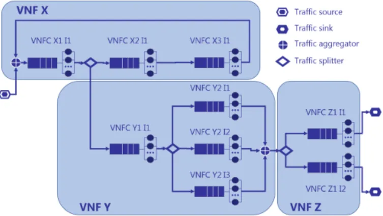
Fig. 1: SNS that is composed of the VNFsX,Y, andZ. VNFs
X,Y, andZ have respectively 3 (e.g.,X1,X2, andX3), 2 (e.g.,
Y1, andY2), and 1 (e.g.,Z1) VNFCs. VNFCsY2andZ1have respectively 3 and 2 instances.
network calculus theory to derive the worst-case performance. Unlike the model proposed in this paper, that one is not applicable to SNSs with feedback such as network control planes. Besides, only numerical results are provided, but the tightness of the provided performance bounds is not assessed [35]. Yoon and Kamal propose a performance model for an SNS in [33]. Specifically, they employ a mixed multi-class BCMP closed-network to model a service chain and apply the model for the NFV resource allocation problem. They use the iterative algorithm MVA to solve their performance model. The time complexity of the model depends on the number of active flows, which may hinder its applicability in scenarios with a large number of ongoing sessions. Finally, Ye et al. also propose a performance model for an SNS in [34]. They assume the decoupling of different flows in the packet processing in each NFV node to characterize the delay of packets traversing the NFV node as an M/D/1 queue. They evaluate their model through simulation. The models mentioned above rely on approximations such as (σ,ρ)-upper constrained [32] or Pois-sonian [34] arrival processes, deterministic service processes [32], [34] and BCMP networks assumptions [33]. Then, their accuracy remains uncertain due to the lack of experimental validation. In this work, we cover this research gap through experimentally evaluating the tightness of our model in a real scenario.
III. SYSTEMMODEL
Let us assume an SNS consisting of a composition of VNFs (see Fig. 1), where each VNF might be composed of one or multiple VNFCs working together. The different VNFs and VNFCs of the SNS are interconnected through VLs with any associated target performance metrics (e.g., bandwidth and latency). Each VNFC provides a well-defined part of the VNF functionality. In turn, each VNFC may have one or several instances, and each VNFC instance is placed on a single VM on which it runs. Please note that in this work,
we do not address the containerization, which is an OS-level virtualization method. Two different instances of the same VNFC might offer distinct computing performance because of the hardware heterogeneity, or they have a different number of allocated CPU cores. The SNS may serve multiple packet flows, which may follow different routes across the VNFCs instances. The packets enter and leave the SNS through its external interfaces.
Without loss of generality, we consider that all the VNFs of the SNS are running in the same data center (NFV Infrastruc-ture). This data center comprises several PMs interconnected through physical switches (see Fig. 2). Each PM hosts a Virtual Machine Monitor or hypervisor and one or several VNFCs instances running in isolated VMs. The different VMs are configured in bridged mode, i.e., they have their own identity on the physical network. The hypervisor includes a virtual switch (vSw) to interconnect the different VMs hosted on the PM [36]. The vSw steers the incoming packets from the physical Network Interface Card (NIC) to the virtual NIC (vNIC) of the corresponding VM. The reception of a packet at the vNIC generates a software interruption that the guest OS handles when the VM is executed. On the VM side, this interruption triggers the load and execution of a service routine to process the packet headers and finally store the packet in the transport layer queue, located in the random-access memory (RAM) (see Fig. 2), until the VNFC instance reads it for processing [30]. The transmission of packets is conducted by the VM on the opposite path in a similar way.
As described in the introduction, here we only concentrate on SNSs whose constituent VNFCs execute CPU-intensive applications for packet processing. Under this assumption, the CPU becomes the computational resource acting as the bottleneck of the VNFCs. Then, the processing time Tk (i.e.,
waiting and serving times) of any VNFC j depends on the number CPU coresmk allocated to it. We consider that these
CPU cores are dedicated (space-shared policy [10]). Thus, any VNFC instance running in the VM does not experience significant dynamic changes in performance at runtime (no DCR assumption) [9]. Each VNFC instancekruns in parallel as many threads of execution as CPU cores mk are allocated
to it. Furthermore, we assume that the SNS does not apply QoS prioritization, and hence, every VNFC instance reads and processes the packets stored in the transport layer queue se-quentially. That is, as long as there are packets in the transport layer queue (e.g., busy period), each thread keeps repeating the same procedure, i.e., it reads the head-of-line packet from the transport layer queue and performs its processing until the end (run-to-completion threads with work-conserving service process). This behavior implies an FCFS serving discipline.
Given two interconnected VNFCs instances k and i, we define the virtual link delay dki as the time elapsed since the
VNFC instancektransmits a packet until the VNFC instance
i receives it. The virtual link delay between two VNFCs hosted on different PMs include mainly the following latency components:
• The processing time of the protocol stack at the source and the destination.
Physical Machine P1 Physical NIC Hypervisor vNIC RAM Queue CPU Pool vSwitch Physical Machine P3 Physical NIC Hypervisor vSwitch vNIC RAM Queue CPU Pool VNFC Y2 I1 VNFC Z1 I1 VNFC Z1 I2 VNFC Y2 I2 VNFC X1 I1 VNFC X2 I1 Physical Machine P2 Physical NIC Hypervisor vSwitch VNFC Y1 I1 VNFC Y2 I3 VNFC X3 I1 Other SNS Physical Switch
Fig. 2: Possible embedding of the SNS depicted in Fig. 1 into a physical infrastructure that consists of three PMs and a physical switchisinterconnecting them.
Fig. 3: Queuing model for the chain of VNFs shown in Fig. 1.
• The back-end driver processing time and the packet transmission to the pNIC through the virtual bridge at the source physical server and the opposite path at the destination physical server [36].
• The processing, queuing, and transmission delay at every physical switch, and propagation delays of the physical links that support the respective virtual link.
Please note that the virtual link delay between two VNFCs instances hosted on the same PM only includes the latency components described in the first two bullet points.
IV. QUEUINGMODEL FORSNSS
This section explains the queuing model for a chain of VNFs and the QNA method. QNA is the methodology of analysis considered to derive the system response time from the model.
A. Queuing Model
Let us consider an SNS that is composed of J different VNFCs. To model this system, we employ an open network of K G/G/m queuesQ1, Q2,· · · , QK (see Fig. 3). As every
a given VNFC can be instantiated on-demand), each queue represents either a VNFC instance running on a VM or a virtual link. For the sake of illustration, Fig. 3 shows the queuing model associated with the SNS depicted in Fig. 1, has
J = 6 VNFCs and 9 VNFCs instances. Specifically, VNFCs Y2 and Z1 have three and two instances, respectively, whereas the rest of VNFCs have only one instance.
The packet processing procedure at each VNFC instance, described in the previous section, is well captured by a G/G/m queuing node1. Them
k servers of the queuing node kstand
for the threads of the corresponding VNFC instance running in the CPU cores allocated to it. These threads process the packets stored in the transport layer queue in FCFS order, in parallel, and as a work-conserving service process.
The virtual link delays dki are taking into account by
introducing a G/G/1 queue and an infinite server in tandem for each virtual link. The G/G/1 queue represents the main bottleneck of the virtual link, while the infinite server accounts for the rest of the delaysθ(kiV L), i.e., the different propagation delays, and the mean service times experienced by the packet when traverses the virtual link. The previous consideration does not preclude to employ more complex models that might consider all the potential bottlenecks of every virtual link. For simplicity, the queuing nodes associated with the virtual links are not included in Fig. 3.
Regarding the external arrival process to each queueQk, it
is assumed to be a generalized inter-arrival process, which is characterized by its mean λ0k and its Squared Coefficient of
Variation (SCV), calculated as c2
0k =variance/(mean)2.
We consider that all servers of the same queue have an identical and generalized service process, which is also char-acterized by its mean µk (service rate) and its SCV c2sk.
However, servers belonging to different queues may have distinct service processes, even if they pertain to the same VNFC. This feature is useful to model the heterogeneity of the physical hardware, underlying the provisioned VMs, inherent to non-uniform infrastructures like computational clouds [9].
Furthermore, every queue has associated a parameter νk,
which is a multiplicative factor for the flow leaving Qk that
models the creation or combination of packets at the nodes. That means that if the total arrival rate to queue Qk is λk,
then the output rate of this queue would be νkλk.
For the transitions between queues, we assume probabilistic routing where the packet leaving Qk is next moved to queue
Qi with probabilitypki or exits the network with probability
p0k = 1−P K
i=1pki. We also consider the routing decision
is made independently for each packet leaving queue Qk.
Please note that although here we are considering probabilistic routing, QNA method, which is the methodology used to solve the resulting network of queues, also includes an alternative analysis for multi-class with deterministic routing [11], [16].
The transition probabilities pki are gathered in the routing
matrix denoted as P = [pki]. This approach allows to define
any arbitrary feedback between VNFC instances and to model
1In Kendall’s notation, a G/G/m queue is a queuing node withmservers, arbitrary arrival and service processes, FCFS (First-Come, First-Served) discipline, and infinite capacity and calling population.
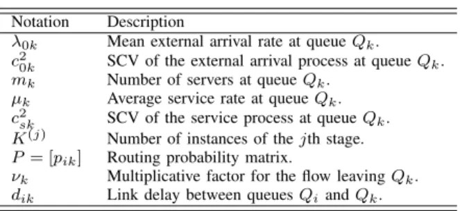
TABLE I: Model input parameters.
Notation Description
λ0k Mean external arrival rate at queueQk.
c2
0k SCV of the external arrival process at queueQk.
mk Number of servers at queueQk.
µk Average service rate at queueQk.
c2
sk SCV of the service process at queueQk.
K(j) Number of instances of thejth stage.
P = [pik] Routing probability matrix.
νk Multiplicative factor for the flow leavingQk.
dik Link delay between queuesQiandQk.
caching effects and different load-balancing strategies at any VNFC.
B. System Response Time
To compute the system response time, we use the QNA method which is an approximation technique [11]. The QNA method uses two parameters, the mean and the SCV, to characterize the arrival and service time processes for every queue. Then, the different queues are analyzed in isolation as standard GI/G/m queues.
Finally, to compute the global performance parameters, the QNA method assumes the queues are stochastically indepen-dent, even though the queuing network might not have a product-form solution. Thus, QNA method can be seen as a generalization of the open Jackson’s network of M/M/m queues to an open Jackson’s network of GI/G/m queues. In fact, QNA is consistent with the Jackson network theory, i.e., if all the arrival and service processes are Poisson, then QNA is exact [11].
As we will show in Section VII-B, although the QNA method is approximate, it performs well to estimate the global mean response time of a VNF. In the following subsections, we describe the main steps of the QNA method in detail. Additionally, Table I summarizes the input parameters of our model, whereas Table II contains the primary notation used through the article.
1) Internal Flows Parameters Computation: The first step of the QNA method is to compute the mean and the SCV of the arrival process to each queue.
Let λk denote the total arrival rate to queue Qk. As in
the case of Jackson’s networks, we can computeλk, ∀ {k∈ N|1 ≤ k ≤ K} by solving the following set of linear flow
balance equations: λk =λ0k+ K X i=1 λiνipik (1)
Let c2ak be the SCV of the arrival process to each queue
Qk. To simplify the computation of thec2ak, the QNA method
employs approximations. Specifically, it uses a convex com-bination of the asymptotic value of the SCV (c2
ak)A and
the SCV of an exponential distribution (c2
exp = 1), i.e.,
c2
ak=αk(c2ak)A+ (1−αk).
The asymptotic value can be found as (c2ak)A =
PK
i=1qikc2ik, where qik is the proportion of arrivals to Qk
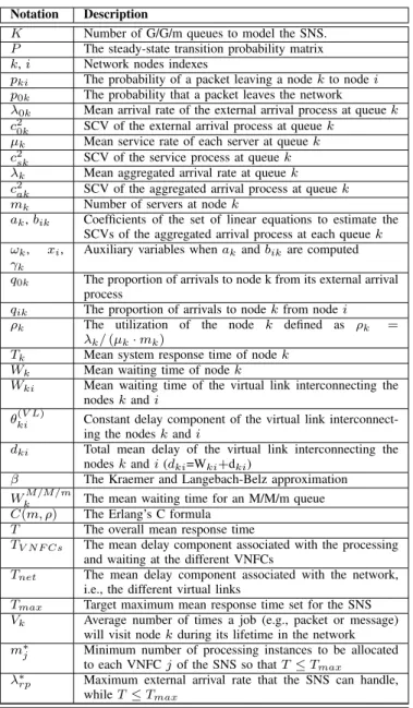
TABLE II: Primary notation.
Notation Description
K Number of G/G/m queues to model the SNS.
P The steady-state transition probability matrix
k,i Network nodes indexes
pki The probability of a packet leaving a nodekto nodei
p0k The probability that a packet leaves the network
λ0k Mean arrival rate of the external arrival process at queuek
c2
0k SCV of the external arrival process at queuek
µk Mean service rate of each server at queuek
c2sk SCV of the service process at queuek λk Mean aggregated arrival rate at queuek
c2
ak SCV of the aggregated arrival process at queuek
mk Number of servers at nodek
ak,bik Coefficients of the set of linear equations to estimate the SCVs of the aggregated arrival process at each queuek ωk, xi,
γk
Auxiliary variables whenakandbikare computed
q0k The proportion of arrivals to node k from its external arrival process
qik The proportion of arrivals to nodekfrom nodei
ρk The utilization of the node k defined as ρk =
λk/(µk·mk)
Tk Mean system response time of nodek
Wk Mean waiting time of nodek
Wki Mean waiting time of the virtual link interconnecting the nodeskandi
θ(kiV L) Constant delay component of the virtual link interconnect-ing the nodeskandi
dki Total mean delay of the virtual link interconnecting the nodeskandi(dki=Wki+dki)
β The Kraemer and Langebach-Belz approximation
WkM/M/m The mean waiting time for an M/M/m queue
C(m, ρ) The Erlang’s C formula
T The overall mean response time
TV N F Cs The mean delay component associated with the processing and waiting at the different VNFCs
Tnet The mean delay component associated with the network, i.e., the different virtual links
Tmax Target maximum mean response time set for the SNS
Vk Average number of times a job (e.g., packet or message) will visit nodekduring its lifetime in the network
m∗j Minimum number of processing instances to be allocated to each VNFCjof the SNS so thatT ≤Tmax
λ∗rp Maximum external arrival rate that the SNS can handle, whileT ≤Tmax
a function of the server utilization ρk = λk/(µk ·mk) and
the arrival rates. This approximation yields the following set of linear equations, which may be solved to getc2
ak, ∀ {k∈ N|1≤k≤K}: c2ak=ak+ K X i=1 c2aibik, 1≤k≤K (2) ak = 1 +ωk (q0kc20k−1) + K X i=1 qik[(1−pik) +νipikρ2ixi] (3) bik=ωkqikpikνi(1−ρ2i) (4) xi= 1 +m−i0.5(max{c 2 si,0.2} −1) (5) ωk = 1 + 4(1−ρk)2(γk−1) −1 (6) γk = K X i=0 qik2 !−1 (7) The most interesting feature of the QNA method is that it estimates the SCV of the aggregated arrival process to each queuec2
ak from the above set of linear equations.
2) Response Time Computation per Queue: Once we have foundλk andc2ak for all internal flows, we can compute the
performance parameters for each queue, which are analyzed in isolation (i.e., considering that the queues are independent of each other).
LetWk be the mean waiting time at queue Qk. Then, the
mean response time at queueQk is given byTk =Wk+1/µk.
IfQk is a GI/G/1 queue (Qk has only one server),Wk can
be approximated as: Wk = ρk·(c2ak+c 2 sk)·β 2·µk(1−ρk) (8) with β= ( exp(−2·(1−ρi)·(1−c2ai)2 3·ρi·(c2ai+c2si) ) c2 ai<1 β = 1 c2 ai≥1 (9) If, by contrast,Qk is a GI/G/m queue,Wk can be estimated
as: Wk = 0.5· c2ai+c 2 si ·WkM/M/m (10)
whereWkM/M/mis the mean waiting time for a M/M/m queue, which can be computed as:
WkM/M/m= C(mk,
λk µk) mkµk−λk
(11) andC(m, ρ)represents the Erlang’s C formula which has the following expression: C(m, ρ) = (m·ρ)m m! · 1 1−ρ Pm−1 k=0 (m·ρ)k k! + (m·ρ)m m! · 1 1−ρ (12)
3) Global Response Time Computation: For the overall mean response time of the SNS, T, we can distinguish two delay contributions, e.g., the overall mean sojourn time associated with the waiting and processing at the VNFCs instances,TV N F Cs, and the overall mean sojourn time of the
network,Tnet. More specifically, Tnet denotes the total time
that any packet spends in the virtual links during its lifetime in the SNS. Then: T =TV N F Cs+Tnet (13) TV N F Cs= K X k=1 (Wk+ 1 µk )·Vk (14) Tnet= K X k=1 K X i=1 dki·pki·Vk = K X k=1 K X i=1 Wki+θ (V L) ki ·pki·Vk (15)
Where Vk denotes the visit ratio for VNFC instance k (Qk)
Qk by a packet during its lifetime in the network. That is
Vk = λk/(P K
k=1λ0k). And, Wki is the waiting time of
the bottleneck in the virtual link interconnecting the VNFC instancesk andi, which can be estimated using (8).
V. PARTICULARUSECASE:ATHREE-TIER VMME The MME is the central control entity of the LTE/Evolved Packet Core (EPC) architecture. It interacts with the evolved NodeB (eNB), Serving Gateway (S-GW), and Home Sub-scriber Server (HSS) within the EPC to realize functions such as non-access stratum (NAS) signaling, user authenti-cation/authorization, mobility management (e.g., paging, user tracking), and bearer management, among many others [13].
In this section, we first motivate the vMME decomposition and describe its operation. Next, we particularize our model to a vMME with a three-tier architecture whose operation is described in [12].
A. vMME decomposition
The VNFs decomposition is of paramount importance for exploiting all the advantages NFV offers. Under this paradigm, a VNF is decomposed into a set of VNFCs, each of which implements a part of the VNF functionality. The way the VNFCs are linked is specified in a VNF Descriptor (VNFD). The VNFs decomposition brings a finer granularity, which might entail some advantages such as better utilization of the computational resources, higher robustness of the VNFs, or to ease the embedding of the VNFs. However, these advantages come at the cost of increasing the complexity of NFV orchestration.
In [37], Taleb et al. describe a1:N mapping option (also referred to as multi-tier architecture), inspired by web ser-vices, for the entities of the EPC. In this mapping, each EPC functionality is decomposed into multiple VNFCs of the following three types: front-end (FE), stateless worker (W), andstate database(DB). Each VNFC instance is implemented in one running virtualization container like a VM. This VNF decomposition has several advantages like higher scalability and availability of the VNF, and it reduces the complexity of VNF scaling [37].
However, the 1:N mapping approach might increase the VNF response time as every packet has to pass through several nodes. That is the main reason why this kind of VNF decomposition has been considered mainly to virtualize control plane network entities, where the delay constraints are less stringent than in the data plane. Several works consider the1:N mappingarchitecture to virtualize an LTE MME [12], [38], [13]. It is also applied to virtualize the IP Multimedia Subsystem (IMS) entities [39].
B. Three-tier vMME Operation
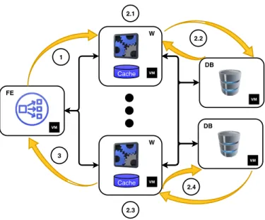
In this subsection, we describe the operation of a vMME with a 1:3 mapping architecture inspired by web services. Figure 4 presents the considered vMME architecture, together with its main operation steps.
The FE is the communication interface with other LTE entities (e.g., eNB, S-GW, and HSS) and balances the load
Cache FE W DB Cache W DB 1 3 2.1 2.2 2.3 2.4
Fig. 4: Architecture and operation of a three-tiered vMME.
among the Ws. Each worker implements the logic of the MME, and the DB contains the User Equipment (UE) session state making the Ws stateless.
The FE acts as the communication interface with the outside world. Thus all packets enter the vMME at the FE with a mean rateλ0F E. Then, the FE sends the packet to the corresponding
W according to its load-balancing scheme (labeled as ”1” in Figure 4). According to the operation described in [12] and [38], the FE tier balances signaling workload equally among the W instances on a per control procedure basis. The FE sends to the same W instance all control messages associated with a given control procedure and UE. We assume that the W instance has enough memory to store all the necessary state data (e.g., UE context) to handle a control procedure during its lifetime.
Once the packet arrives at the W, it parses the packet and checks whether the required data for processing the packet are stored in its cache memory (labeled as ”2.1” in Figure 4). This cache memory could be implemented inside the RAM allocated to the VM, where the W is running on. If a cache mismatch occurs, then the W forwards a query to the DB to retrieve the data from it (labeled as ”2.2” in the same figure). Please note that this data retrieval pauses the packet processing at the W, during which the W might process other packets.
When the DB gathers the necessary state variables, it sends them encapsulated in a packet back to the W. The W can then finalize the packet processing (labeled as ”2.3” in Figure 4). After processing finishes, it might be necessary to update some data in the DB (labeled as ”2.4”). Then, the W generates a response packet and forwards it to the FE (labeled as ”3”). Finally, the packet exits the vMME.
Here, we consider that the W will retrieve the UE context from DB when the initial message of a control procedure arrives. Furthermore, the W will save the updated UE context into the DB when the W finishes processing the last message
vMME
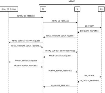
Fig. 5: Three-tiered vMME call flow for handling the service request signaling procedure.
Fig. 6: Queuing model for the vMME with a three-tier design shown in Fig. 4 .
of a signaling procedure [12] [38]. Figure 5 illustrates the messages exchanged between the different virtualized Mobil-ity Management EntMobil-ity (vMME) components for handling a service request procedure.
C. Queuing Model for the vMME
Figure 6 depicts the queuing model associated with the three-tiered vMME shown in Fig. 4. As previously mentioned, this model is a particular case of the performance modeling approach described in Section IV. More precisely, we model the vMME as an open network of G/G/m queues, where each queuing node represents an instance of a given VNFC (e.g., FE, W, DB) of the vMME. The model comprises
K = KF E +KW +KDB G/G/m queues, where KF E,
KW, andKDB denote the number of front-end, worker, and
database instances, respectively. The servers of a queuing node represent the CPU instances, allocated to the corresponding VNFC instance, processing control messages in parallel.
The traffic source and sink are respectively located at the input and output of the FE instances, as the FE tier is the external interface with the rest of the network.
1) Signaling Workload for the vMME: The UEs run ap-plications that generate or consume network traffic. This
UE activity and mobility trigger the LTE network control procedures. These signaling procedures allow the control plane to manage the UE mobility and the data flow between the UE and Packet Data Network Gateway (P-GW). Each of these control procedures yields several signaling messages to be processed by the vMME.
Here, we only consider the most frequent LTE signaling procedures, e.g., Service Request (SR), S1-Release (S1R), and X2-Based Handover (HR) [40].
LetfCP andnCP respectively denote the relative frequency
of occurrence and the number of packets to be processed by the MME for each control procedureCP ∈ {SR, S1R, HR}. Specifically, nSR = nS1R = 3 and nHR = 2. Then, we
can compute the average number of packets per signaling procedureNpp as
Npp=
X
CP
fCP ·nCP = 3·fSR+ 3·fS1R+ 2·fHR (16) 2) Transition Probabilities: We assume perfect load bal-ancing for all tiers [41]. That is, each FE, W, and DB instance respectively processes 1/KF E, 1/KW, and 1/KDB fraction
of the total workload of the tier they belong to.
According to the vMME operation described in [12], there are two DB accesses per control procedure. Therefore, the visit ratio per packet at each DB and W instance will respectively
beVDB = 1/KDB·2/Npp andVW = 1/KW ·(1 + 2/Npp).
The FE maintains 3GPP standardized interfaces towards other entities of the network (e.g., eNBs, HSS, and S-GW). Thus all the control messages are processed by the FE tier two times: once when they enter the vMME and one before they leave it. We can model this process by considering that each packet served at any FE instance leaves the vMME (queuing network) with probability p0F E = 0.5. That is because half
of all packets arriving at any FE instance will exit vMME (queuing network). As mentioned, each packet visits the FE tier two times. Thus its visit ratio equals two. Considering we have KF E instances and the workload is equally distributed
among them, the visit ratio of each FE instance is given by
VF E= 2/KF E.
Consequently, the transition probabilities between the VNFC instances of the vMME are given by:
pF E→W = 1 KW · 1 2 (17) pW→F E= 1 KF E · 1 (1 +N2 pp) (18) pW→DB= 1 KDB · 2 Npp (1 + N2 pp) (19) pDB→W = 1 KW (20) VI. EXPERIMENTALPROCEDURES
In this section, we present our experimental setup, the procedures used to measure the input parameters for the model, and a description of the experiments carried out to measure the response time of the three-time vMME described in the previous section.
A. Experimental Setup
To validate our model, we developed the following software tools: i) a traffic source, ii) an LTE network emulator, and iii) a vMME with a three-tier design. All of these tools were implemented in C/C++.
The traffic source generates LTE procedure calls according to the compound traffic model and the scenario considered in [13]. It only emulates the triggering of the most frequent LTE signaling procedures (e.g., Service Request, S1-Release, and X2-based handover) [40]. The minimal inter-departure time supported by the traffic source is5 µs.
The LTE network emulator reproduces the eNodeB and S-GW behavior. It processes and generates the signaling mes-sages the eNB and S-GW would exchange with the vMME. It also emulates the latencies between the vMME and these LTE network entities by introducing a constant delay to every incoming and outgoing packet. For all the experiments carried out, the two-way delay between the vMME and network emulator was set to 9 ms, which we expect to be within the range of round trip times from an MME in an LTE commercial network. The three-tier vMME follows the behavior described in Section V. Although our implementation is not fully 3GPP compliant, it performs similar operations. The database tier was implemented by using SQLite 3 entirely loaded in RAM. Regarding the hosting environment, our experimental frame-work includes different kinds of physical servers. There are three servers with Intel(R) Core(TM) i7-6700K CPU at 4.00GHz with 4 core, which are referred to astype I servers. And one server with two Intel(R) Xeon(R) E5-2603 CPUs at 1.70GHz, with 6 cores each, which is referred to as type II
server. All the servers have a 10 Gbps Ethernet NIC, 32 GB of RAM, and run Ubuntu Server 16.0. All these servers are interconnected through an 8-port 10 Gbps Ethernet switch.
For the virtualization environment, we used Kernel-based Virtual Machine (KVM) for the Linux kernel. Each of the physical servers runs a KVM hypervisor [42]. For all KVM guests, the NICs were paravirtualized with the Linux standard
virtio, and bridged networking was used [42]. In our experi-ments, each VNFC instance of the vMME (e.g., FE, W, and DB) runs on a different VM. The VMs hosting the FE and DB instances run on separated type I servers, whereas the VMs hosting the W instances run on the type II server. The traffic source and network emulator run on the other type I server.
In order to enhance vMME performance, we set several CPU related configurations [43]. Explicitly, we disabled the hyperthreading feature, the dynamic frequency scaling gover-nor, and the processor C-States. Also, we used CPU pinning and configured the affinity of the processes in order to allocate one dedicated physical core to each VNFC instance [42].
The Linux kernel version 4.4.0-81-generic default settings were used for all the networking buffers, e.g., the receive
rmem default and send wmem default socket buffers were fixed at 212992 bytes; and the buffer reception at any interface,
netdev max backlog, was fixed at 1000 packets. With this setting, a negligible probability of packet loss was observed in all our experiments.
B. Parameter Estimation
This section explains the methodology and procedures used to estimate the input parameters (see Table I).
1) External arrival process: We estimated it by recording the arrival times of the packets at the external interfaces of the VNF. Samples of the inter-arrival time, IAT, can be obtained as the difference between the arrival instants of two consecutive packets. Then, the first and second-order moments,
E[IAT] = 1/λ0andV AR[IAT] =ca20·E[IAT]2, ofIAT can
be respectively estimated as the sample mean and variance.
2) Service processes: We characterized the service process for each VNFC by taking measurements of the service time directly from the source code of the application. That is, by reading the system clock at the beginning and the end of the execution of the code which implements the packet processing. Samples of the service time, sk, were taken for
every processed packet at the VNFC instance k. Then, we estimated the first and second-order moments, E[sk] = 1/µk
andV AR[sk] =c2sk·E[sk]2, ofsk as the sample mean and
variance.
In order to ensure that the above measurements are good approximations of the actual service time at any VNFC instance, the following measurement process was tried. With the VNFC instance sufficiently overloaded (i.e., the queue is never empty), we monitored and recorded the departure times of the outgoing packets. Then actual samples of the service time can be obtained as the difference between the departure instants of two consecutive outgoing packets. This estimation allows us to consider the VNFC as a black box, i.e., the source code is not required.
We carried out an experiment where we estimated the service time process of a VNFC instance by using both techniques above. The values measured for the mean and SCV of the service time were 155.08 µs and 1.06, respectively, by using the first methodology, and 157.29 µs and 1.03, respectively, with the second one. Hence, we conclude that both measurement methods provide similar results in the considered scenario.
3) Transition probabilities: As mentioned in Section V-C2, in our case, the probability transition matrix (or equivalently the visit ratios) depends on the VNF internal operation and the percentages of each type of LTE control procedure. Since we know the VNF internal operation beforehand, we only needed to monitor the frequency of occurrence of each considered signaling procedure,fCP, at the front-end.
In a more general scenario, the transition probability matrix can be estimated by using counters at each VNFC instance to monitor the number of incoming packets and the outgoing packets towards other VNFC instances.
4) Virtual link delays: In our experimental setup, there was no mechanism to synchronize the clock of the different physical servers. Then, in order to estimate the virtual link delays, dki, between the VNFC instances k and i, we
em-ployed an echo service. Let us assume we want to measure
dki, and the echo server is running in the same VM as i.
At the VNFC instance k, the departure time of the query message,Q(kout), and the arrival time of the response message,
R(kin), were recorded. At the VNFC instancei, the arrival and departure instants of the query and response messages, Q(iin)
and R(iout), were collected. Then, we assumed symmetric virtual links betweenkandi, i.e.,dki=dik, and estimated the
virtual link delay,dki, between kandias the sample average
(1/2)·Rk(in)−Q(kout)−Ri(out)−Q(iin).
C. Experiments
We considered five scenarios with 1, 2, 3, 4, and 5 worker instances, respectively. We refer to these scenarios asS1,S2,
S3, S4, and S5, respectively. There was only one database and front-end instance for all of them. Several signaling workload points were evaluated for each of them. Specifically, we assessed 10, 11, 13, 16, and 19 workload points for S1,
S2, S3, S4, and S5, respectively. The maximum signaling workload evaluated for S5 was 17000 control packets per second. Each experiment, i.e., a signaling workload point for a given scenario, was repeated 5 times. The processing of 200000 by the vMME was the stop condition for all the validation experiments.
The measurement tools employed in all our experiments were network sniffers monitoring the incoming and outgoing traffic at the vNIC of the VM hosting each VNFC instance. To measure the vMME response time, we recorded the arrival time of each control message and the departure time of its corresponding response at the FE instance.
VII. EXPERIMENTALRESULTS
In this section, we validate the proposed QT-based per-formance model for a vMME with a 1:3 mapping archi-tecture. For this purpose, we provide the results from the analytical model and compare them with the results obtained from our experimental testbed. In addition, we compare the QNA method [11] with the Jackson’s networks and MVA methodologies. We chose these methodologies because they are the standard methodologies employed in queuing theory to solve a network of queues. To the best of our knowledge, all the related works using a performance modeling approach based on queuing networks rely on those methodologies.
A. Measured Input Parameters for the Model
Figure 7 depicts the measured service time distribution for each VNFC, i.e., the time required by a processing instance for processing allocated to the respective VNFC for processing a single control message.
The results show that the FE, W, and DB service times present a ladder shape. This behavior is because each tier type has to carry out different processing tasks depending on the kind of incoming packet, as described in [14]. More precisely, the FE has to run the load balancing strategy for the incoming packets to the vMME, but not for the outgoing packets. The DB has to process two different classes of packets, e.g., queries and updates. Last, the W tier has to execute a specific code to each kind of control message. Leaving aside the specificities for processing each type of message, we observed there are operations with a high computational burden in our
W implementation that significantly influence the shape of the W service time distribution FsW. Those operations are
the encryption and integrity protection of the packets and the W cache update. On the one hand, the security-related operations affect roughly 60% of the total number of packets processed by the W VNFC, as our W implementation does not encrypt and does not provide integrity protection for the packets exchanged with the DB tier (e.g., DB_QUERY and
DB_UPDATE). On the other hand, the W cache update is
only carried out after receiving the DB_QUERY_RESPONSE
message (refer to Fig. 5), thus it approximately affects 20% out of the total number of packets processed by the W. This fact explains the two particularly evident jump discontinuities of FsW when FsW ≈0.4 andFsW ≈0.8.
Although the fact described above is the primary source of variability in the service processes, their distributions present non-negligible tails (see Fig. 7). Despite the CPU related settings configured (e.g., CPU pinning, and disabling the hyperthreading, frequency scaling governor, and processor C-states), the virtualization environment does not provide a real-time operation for the hosted VNFCs instances. For instance, there are still kernel-level processes sharing the CPU cores with the VNFCs instances. These processes might eventually interrupt the execution of the VNFC instance and inflate the service time of its ongoing control messages during a busy period.
Interestingly, the tail of the FE service time is longer than the DB one, though both tiers run on the same type of PM (type Iserver). The explanation of this phenomenon might be associated with the fact that the FE has to process 2.76 times more control messages than the DB in our setup. In other words, the realization of the FE service process showed in Fig. 7 was estimated using 2.76 times more samples than the DB one. Then, it is more likely to observe rare events (e.g., kernel-level processes disrupting the VNFC instance execution for more extended periods) in the FE service time distribution. From the sample mean and variance of the application service time collected from our experimental testbed, we estimate the service rate µ and the SCV c2
s (see Table III).
These values are provided with a 95% confidence interval. The results show that the FE application has the highest service rate, whereas the W has the lowest service rate of all considered VNFCs. This fact is the motivation behind the horizontal scaling of the W VNFC.
Additionally, we have measured the virtual link delay dki
between different VNFC instances (see Table III) from our testbed up to a rate of 17000 packets per second. The mea-surements have yielded a nearly constant mean delay within the evaluated range.
Finally, we estimated the transition probabilities between VNFCs using (16), (17), (18), (19), and (20) (see Table III). As shown in Section V-C, for our case, they only depend on the VNF internal operation and the frequency of occurrence for each type of control procedure. For all our experiments,fSR≈
fSRR ≈0.44 andfHR≈0.12. Consequently, the visit ratio
of each VNFC instance areVF E = 2,VW = (1/KW)·1.69,
TABLE III: Measured input parameters for the model.
Service Processes
FE service rate (µF E) 115126 packets per second FE service time SCV (c2sF E) 0.0225±0.0088 W service rate (µW) 6716 packets per second W service time SCV (c2
sW) 0.6457±0.0016
DB service rate (µDB) 23874 transactions per second DB service time SCV (c2 sDB) 0.0280±0.0001 Transition Probabilities pF E→W K1W·0.5 pW→F E 0.59 pW→DB 0.41 pDB→W K1W
Virtual Link Delays
dF E→W =dW→F E 29.54±0.22µs dW→DB=dDB→W 31.33±0.38µs Service time (7s) 100 101 102 103 CDF 0 0.2 0.4 0.6 0.8 1 Front-end Worker Database
Fig. 7: Service time process for each VNFC.
B. Model Validation
In order to validate the parameters of the arrival processes for each VNFC instance, first, the relative error between the estimation of the SCVs of the internal arrival processes c2ak, provided by (2), and the measured SCVs was computed. A relative error sample was computed for each tested external arrival rate, and each scenario (from 1 to 5 workers) and minimum, maximum, average, and standard deviation values were calculated with these samples, see Table IV. As shown, the average error is approximately 26%, 24%, and 8.5% for the FE, the Ws, and the DB, respectively. We have observed that, for each scenario, the estimation error decreases with the load. One potential approach to enhance the accuracy in the estimation of the SCVs of the internal arrival processes might be the use of predictive Machine Learning-based techniques. For instance, an artificial neural network could be trained through simulation to predict the SCVs, depending on the setup of the system.
Fig. 8 shows the overall mean response time of the vMME,
T, obtained experimentally (labeled as ’Exp’) and computed using our model (labeled as ’QNA’) and the method for analyzing Jackson’s networks (labeled as ’Jackson’). As in
TABLE IV: Characterization of the relative error for the estimation of the SCVs of the internal arrival processes.
VNFC min max avg sdt
FE 2.29% 62.30% 26.20% 12.50% W 0.03% 63.34% 24.10% 15.74% DB 0.16% 40.88% 8.55% 9.36%
External arrival rate, 60, (packets per second)
0 2000 4000 6000 8000 10000 12000 14000 16000 18000
Mean response time, T, (
7 s) 500 1000 1500 2000 2500 Exp QNA Jackson KW=1 KW=2 KW=3 KW=4 KW=5
Fig. 8: Overall mean system response time.
Worker utilization, ; W, (%) 0 0.1 0.2 0.3 0.4 0.5 0.6 0.7 0.8 0.9 1 Relative error, 0 , (%) 0 10 20 30 40 QNA Jackson
Fig. 9: Model validation.
[14], the MVA algorithm yielded similar results to Jackson’s methodology. Then, for clarity purposes, the corresponding results have not been included in Fig. 8. This figure combines the results from the 5 executed scenarios, i.e., using from 1 to 5 workers. Additionally, each load point is executed 5 times and the mean value, and the 95% confidence intervals are included. As shown, the QNA model closely follows the empirical curve. Similarly, Fig. 9 presents a scatter plot of the relative error for the different analytical models considered. This error is calculated as = |Texp−Ttheo|/Texp, where Texp and
Ttheoare the mean response time obtained experimentally and
computed by using the corresponding model, respectively. As shown, the QNA model outperforms Jackson’s approach for medium and high loads, achieving less than half of error. For low loads, both methods produce an error lower than 10 %.
Please observe that the relative error of both methodologies decreases whenρW >0.8. This result can be explained by the
fact that (8) and (10) were derived by assuming heavy traffic conditions [44]. Then, it is expected that the model performs better whenρW →1. In the same way, Jackson methodology
also performs better, since the mean waiting time of an M/M/m queue is roughly proportional to the actual mean waiting time of a G/G/m queue for heavy loads, see (8) and (10).
C. From Theory to Practice
In this subsection, we showcase the application of the proposed model for the proactive DRP of the three-tiered vMME. The proactive DRP mechanism considered is triggered periodically every∆Tprovunits of time. The DRP mechanism
performs three essential steps:
i) It predicts the maximum external arrival rate to the FE from the current instant until the time scheduled for the next triggering of the DRP mechanism.
iii) If necessary, a provisioning request is issued to scale in/out the vMME components.
Besides, we consider an Admission Control Mechanism (ACM) to decline the excess incoming signaling procedures during unexpected workload surges. The ACM is aware of the maximum workload λrp the vMME can handle at every
instant in order to meet a given mean response time threshold
Tmax. Then, ifλ0F E(t)> λrpat any instant t, the ACM will
reject the new incoming signaling procedures to the vMME. We rely on the following closed-form expression derived in [45] for the resource dimensioning of the SNSs:
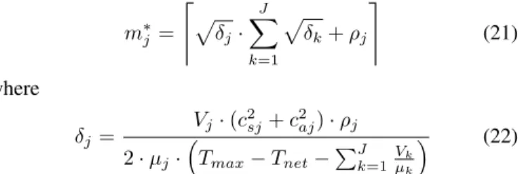
m∗j = & p δj· J X k=1 p δk+ρj ' (21) where δj= Vj·(c2sj+c2aj)·ρj 2·µj· Tmax−Tnet−P J k=1 Vk µk (22)
Equations (21) and (22) enable the estimation of the optimal number of processing instances m∗j to be allocated to each
VNFC j ∈ [1, J] of an SNS so that T ≤ Tmax. Where Vj
denotes the visit ratio to the VNFC j, and c2
aj is the SCV
of the internal arrival process to each instance of the VNFC
j. The rest of the parameters are defined in Section IV. The authors in [45] derive (21) and (22), considering the waiting time at each VNFCjis given by (8). Also, they suppose there is an auxiliary mechanism that can estimatec2aj. To that end, we used (2)-(7).
The maximum workloadλrp that the vMME can handle at
every instant so thatT ≤Tmaxis also estimated from (21) and
(22) given that λj=Vj·λrp for T =Tmax andρj =λj/µj.
Then, λrp=φrp· J ^ j=1 m∗j q δ0 j· PJ k=1 p δ0 k+ Vj µj (23) whereV
stands for the minimum operator, andδj0 is given by:
δj0 = V 2 j ·(c2sj+c2aj) 2·µ2 j· Tmax−Tnet−P J k=1 Vk µk (24)
Please observe we have introduced the new parameter φrp∈
[0,1] in (23) to avoid the SNS reaches the operation point whereT =Tmax. As observed in Fig. 8, the model
underes-timated the mean response time for some experimental runs at high loads (utilizations of 90%). Using (23) and (24), we can properly update the configuration of the ACM after every provisioning decision.
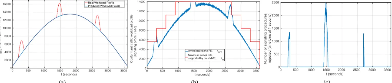
The conducted DRP experiment lasted one hour. We set
φrp = 0.95 and Tmax = 1 ms. Figure 10a shows the
considered workload profile (i.e., mean arrival rate to the vMME over time) labeled as “Real Workload Profile”. The profile resembles the shape of the sinusoidal function with an image between 500 and 13500 signaling procedures per second. Also, we introduced three synthetic workload bursts with a maximum additional rate of3250control procedures per second and 180 seconds of duration. The workload predictor of the DRP mechanism is unaware of those bursts. Specifically,
the workload profile predicted by the DRP mechanism is labeled as “Predicted Workload Profile” in Fig. 10a.
We implemented the request policing of the ACM by using a sliding window rate limiter with a window size of τ = 1
second. Then, the ACM will accept an incoming signaling procedure arriving at time t iff the number of signaling procedures accepted previously during the period t −τ is lower than λrp(t) ·1s. Figure 10b depicts λrp over time
estimated by using (23) and (24), and the workload profile after passing through the ACM (labeled as “Arrival rate to the FEλ0F E”). Last, Fig. 10c shows the number of signaling
procedures rejected per second versus the time. As observed, the ACM prevents the vMME from being overloaded by the sudden bursts of control traffic.
Figure 11 shows the measured vMME mean response time over time. We set ∆Tprov= 300 seconds. The top of Figure
11 includes labels indicating the number of W instances at any time. The vertical dashed lines highlight the time instants at which the DRP mechanism issued scaling requests to instantiate or remove W instances. The vMME mean response time was estimated using a moving average filter with a window size of20000samples. These results prove the validity of the performance model proposed in this work for the DRP of SNSs. As observed, the maximum vMME mean response time is always kept below Tmax= 1 ms.
Last, it is noteworthy to mention that we observed that for some experiments, the vMME violated the performance requirement T ≤ Tmax right after the scale in operation,
i.e., when the number of workers was decreased, at the third unexpected burst (see Fig. 10b). This undesirable behavior is due to the scale in operation took place prematurely when the system was still serving an ongoing high load. A solution to avoid this issue is to delay the scale in operations until the number of ongoing packets in the SNS is lower thanλrp·Tmax
(little’s law), whereλrp here denotes the maximum workload
to be supported by the SNS after the scale in operation.
VIII. CONCLUSIONS ANDFUTUREWORK
In this article, we have proposed and validated an analytical model based on an open queuing network to estimate the mean response time of a Softwarized Network Service (SNS). The proposed model is sufficiently general to capture many of the complex behaviors of such systems. To analyze the queuing network, we adopt the Queuing Network Analyzer method proposed in [11], which is an approximate method to derive the performance metrics of a network of G/G/m queues from the second-order moments of the external arrival and service processes.
We have validated our model experimentally for an LTE virtualized Mobility Management Entity (vMME) with a three-tier design use case. We have shown that the transition probabilities of a three-tiered vMME depend on the fre-quency of occurrence of each LTE control procedure. We have provided a detailed description of our testbed, which includes a typical data center virtualization layer. We also describe the experimental procedures employed to measure the input parameters for the model (e.g., external arrival process,