Improved entropy based test of uniformity using ranked set samples

Transactions

[email protected] ISSN: 1696-2281

eISSN: 2013-8830 www.idescat.cat/sort/

Improved entropy based test of uniformity

using ranked set samples

M. Mahdizadeh and N. R. Arghami∗

Abstract

Ranked set sampling (RSS) is known to be superior to the traditional simple random sampling (SRS) in the sense that it often leads to more efficient inference procedures. Basic version of RSS has been extensively modified to come up with schemes resulting in more accurate estimators of the population attributes. Multistage ranked set sampling (MSRSS) is such a variation surpassing RSS. Entropy has been instrumental in constructing criteria for fitting of parametric models to the data. The goal of this article is to develop tests of uniformity based on sample entropy under RSS and MSRSS designs. A Monte Carlo simulation study is carried out to compare the power of the proposed tests under several alternative distributions with the ordinary test based on SRS. The results report that the new entropy tests have higher power than the original one for nearly all sample sizes and under alternatives considered.

MSC: 62G30; 62F03

Keywords: Information theory, ranked set sampling, test of fit.

1. Introduction

When the sampling units are difficult to measure but are reasonably simple and cheap to order according to the variable of interest, ranked set sampling (RSS) serves as an appealing alternative to the usual simple random sampling (SRS). Examples of this setup can be found in areas such as agriculture, environment and ecology. The RSS design works by ranking randomly drawn sampling units and quantifying a selected subset of them. McIntyre (1952) introduced this sampling technique while studying the yield of pasture in Australia. He suggested that a fairly accurate ordering of a set of adjacent plots by yield can be made using visual perception, although measuring the

* Department of Statistics, School of Mathematical Sciences, Ferdowsi University of Mashhad, P.O. Box 91775-1159, Mashhad, Iran. Corresponding author E-mail address: [email protected]

Received: June 2010 Accepted: December 2010

yield of each plot is expensive. As a similar situation, consider the following example mentioned by Gulati (2004). Suppose it is of interest to count the number of specific bacterial cells per unit volume in a cell suspension. A set of test tubes, containing the cell suspension, can be ordered by concentration using an optical device without actual measurement on them.

The RSS method can be elucidated as follows.

1. Drawkrandom samples, each of sizek, from the target population.

2. Apply judgement ordering, by any cheap method, on the elements of the ith (i=1, . . . ,k) sample and identify theith smallest unit.

3. Actually measure thekidentified units in step 2.

4. Repeat steps 1-3,htimes (cycles), if necessary, to obtain a ranked set sample of sizen=hk.

The set of measured observations makes up a ranked set sample of sizen denoted by

{X[i]j:i=1, . . . ,k;j=1, . . . ,h}, whereX[i]j is theith judgement order statistic from the jth cycle. To have better understanding of difference between the ranked set sample and simple ranked set sample of the same size, we consider the case of single cycle (h=1) and perfect judgement ranking. In this case, the ranked set sample observations are also the respective order statistics. LetX1, . . . ,Xkbe a simple random sample of sizek from

a continuous population with probability density function (PDF) f(x) and cumulative distribution function (CDF)F(x), and letX_[1], . . . ,X_[k]denote a ranked set sample of size

kobtained as described above.

In the SRS case, the k observations are independent and each of them represents a typical value from the population. Letting X₍1)≤. . . ≤X(k) be the order statistics associated with these SRS observations, we note that they are dependent random variables with joint PDF given by

gSRS(x(1), . . . ,x(k)) =k!

k

∏

i=1

f(x₍i)).

In the RSS settings, additional information and structure is provided by through the judgement ranking process. ThekmeasurementsX_[1], . . . ,X[k]are also order statistics but in this case they are independent observations and each of them provides information about a different aspect of the population. The joint PDF forX_[1], . . . ,X_[k]is given by

gRSS(x[1], . . . ,x[k]) =

k

∏

i=1

fi(x[i]),

where fi(.) is the PDF for theith order statistic of a simple random sample of size k

the independence of the resulting order statistics that enables RSS-based procedures to be more efficient than their RSS competitors with the same number of quantified units. A detailed discussion on the theory and applications of RSS can be found in the recent book by Chen et al. (2004).

Consider estimating the population mean under the aforesaid designs. Let ¯XSRS=

∑k_i=1Xi/kand ¯XRSS=∑ki=1X[i]/kbe the SRS and RSS sample mean, respectively. Hence, we have E(_X¯_{RSS) =} 1 k k

∑

∑

Since the summation in equation (1) is just the sum over entire sample space of the probabilities for a binomial random variable with parametersk−1 andF(x), it follows that

E(_X¯_{RSS) =}Z ∞

−∞x f

(x)dx=µ.

Lettingµ_[i]=E(X[i]), fori=1, . . . ,k, we note that

E(X[i]−µ)2=E(X[i]−µ_[i]+µ_[i]−µ)2=E(X[i]−µ_[i])2+ (µ[i]−µ)2,

since the cross-product terms are zero. So

Var(_X¯_{RSS) =} 1 k2 k

∑

∑

Now, proceeding as we did with E(_X¯_{RSS), we see that}

k

∑

∑

∑

Once again, using the binomial expansion, the interior sum is equal to 1 and we obtain

k

∑

Combining equations (2) and (3) yields Var(_X¯_{RSS) =}σ2 k − 1 k2 k

∑

Al-Saleh and Al-kadiri (2000) extended the usual concept of RSS to to double ranked set sampling (DRSS) with the aim of constructing improved estimators of the population as compared with those associated with RSS and SRS. Subsequently, Saleh and Al-Omari (2002) introduced multistage ranked set sampling (MSRSS), as a generalization of DRSS, and showed that estimators based on MSRSS dominate those obtained by DRSS. The MSRSS scheme can be summarized as follows.

1. Randomly identify kr+1 units from the population of interest, where r is the number of stages.

2. Allot thekr+1units randomly intokr−1sets ofk2units each.

3. For each set in step 2, apply 1-2 of RSS procedure explained above, to get a (judgement) ranked set of size k. This step gives kr−1 _{(judgement) ranked sets,} each of sizek.

4. Without actual measuring of the ranked sets, apply step 3 on thekr−1_{ranked set to} gainkr−2second stage (judgement) ranked sets, of sizekeach.

5. Repeat step 3, without any actual measurement, until an rth stage (judgement) ranked set of sizekis acquired.

6. Actually measure thekidentified units in step 5.

7. Repeat steps 1-6,htimes, if necessary, to obtain anrth stage ranked set sample of sizen=hk.

In analogy with the previous notation, therth stage ranked set sample will be denoted by{X_[(_ir_])_j :i=1, . . . ,k;j=1, . . . ,h}. Two special cases of r=1 and r=2 in MSRSS coincide with RSS and DRSS, respectively.

Goodness-of-fit tests are used to decide whether an observed sample can be consid-ered as a set of independent realization from a given CDFF0. More precisely, they are used to test the hypothesisH0:F=F0, withF being the true CDF of the observations. For a review of goodness-of-fit tests based on SRS refer to the book by D’Agostino and Stephens (1986). Testing hypotheses on the parameters of classical distributions using ranked set samples have been developed in a large number of papers. However, this is not true in the case of test of fit, and a limited number of works are available on this topic. Stokes and Sager (1988) exploited RSS in estimating CDF. They proposed RSS analogue of Kolmogorov-Smirnov (KS) test and derived the null distribution of the test statistic.

Some distributions like normal, exponential and uniform have received much atten-tion in the literature because of their tractable mathematical form. This is true in the

case of RSS and its variations. For example, estimation of parameters and quantiles of uniform distribution using generalized ranked-set sampling have been investigated (e.g., Adatia, 2003; Adatia and Ehsanes Saleh, 2004). In practical situations, however, the dis-tributional form of the population is rarely known. Thus, application of these customized inferential methods is dependent on the availability of appropriate testing procedures for the assumptions of uniformity. Given a sample size, relative precision (RP) of the RSS estimator of the population mean with respect to its SRS counterpart (defined as the variance of the SRS mean divided by the variance of the RSS mean) differs according to the underlying distribution of the data, and is bounded above by(k+1)/2 for continu-ous distributions (1<RP<(k+1)/2) (wherekis the set size with which the ranked set sample is collected), with the upper bound achieved only for the uniform distribution. We may be interested to know whether the RSS has the highest efficiency over SRS in estimating the population mean in a specific situation. This could be another reason for developing uniformity test based on RSS.

As an information-theoretic measure of uncertainty, Shannon (1948) proposed en-tropy of a distribution, and proved that the enen-tropy of normal distribution exceeds that of any other distribution with a density having the same variance. Vasicek (1976) used this property to introduce a test of the composite hypothesis of normality, and impressed de-velopment of tests of fit for other distributions. Such entropy-based tests of fit are avail-able for some other distributions. See Dudewicz and van der Meulen (1981), Gokhale (1983), Grzegorzewski and Wieczorkowski (1999), and Mudholkar and Tian (2002). In this paper, we tackle the problem of testing uniformity, with an entropy-based approach, when the researcher obtains data using RSS and MSRSS. Similar procedures for the inverse Gaussian law was suggested by Mahdizadeh and Arghami (2010).

The paper proceeds as follows. In Section 2, some basic notions from information theory are reviewed, entropy based tests of uniformity based on RSS and MSRSS are suggested, and critical values of the respective test statistics are provided for some sample sizes. Power properties of the new tests are assessed by means of simulations whose results are reported in Section 3. A summary completes the paper in Section 4.

2. The tests

Entropy of a distributionF(x)with density function f(x)is defined as

H(f) =−

Z ∞

−∞ f(x)logf(x)dx. (4) Vasicek (1976) presented a nonparametric entropy estimator forH(f)based on spacings of sample order statistics. The estimator called sample entropy is given by

Vm,n(fX) = 1 n n

∑

where X₍1), . . . ,X(n) are the ordered values of a random sample of size n from F,

X(j)=X(1), if j<1, X(j)=X(n), if j>n and the window sizemis a positive integer such thatm≤n/2. This estimator is derived by expressing (4) in the form

H(f) = Z 1 0 log d duF −1_(u) du,

replacing the distributionFby the empirical distribution function, and using a difference operator instead of the differential operator.

Since entropy estimator (5) is based on spacings, one would need ordered values of the ranked set sample to estimate entropy in RSS. Imitating the SRS case, we first pool the units in all cycles and then form the estimator based on the ordered pooled sample. The MSRSS analogue ofVm,n(fX)turns out to be

V_m(r_,)_n(fX) = 1 n n

∑

whereX₍(_ar₎) is the ath(a=1, . . . ,n) order statistic of therth stage ranked set sample. From now on, the estimator (5) will be denoted byVm(0,n)(fX).

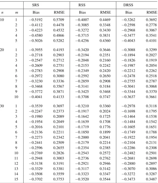
A simulation study was undertaken to compare the proposed estimators of entropy when the uniform U(0,1) is the underlying distribution. Table 1 displays simulated biases and root mean square errors (RMSEs) ofVm(r,n) forr=0,1,2 based on 10,000 samples

with n=10,20,30, and k =10 in MSRSS design (this setup is retained throughout the paper). It is seen that MSRSS improves entropy estimation with respect to SRS for givenmandn. Besides, as the stage number increases, the absolute bias, and RMSE of the corresponding estimator diminishes.

Consider a random sampleX1, . . . ,Xn from a population having a density function f with the support (0,1) and suppose it is of interest to verifyH0:X∼U(0,1) versus

H1:∼H0. It is well-known that for an f concentrated on (0,1) we haveH(f)≤0, and the maximum value ofH(f)is uniquely attained by the U(0,1) density (see Ash, 1965). Based on this result, Dudewicz and van der Meulen (1981) developed a test ofH0. Their test procedure is alternatively defined by the critical region

Tm,n(fX) =exp Vm,n(fX)

≤Tm∗,n,α(fX),

whereTm∗,n,α(fX) is the 100α percentile of the null distribution of Tm,n(fX). It can be shown, using convexity and Jensen’s inequality, thatVm,n(fX)≤0 for all f on (0,1).

Table 1: Simulated biases and RMSEs of Vm(r,)n(f)(r=0,1,2)

for the U(0,1) distribution with H(f) =0.

SRS RSS DRSS

n m Bias RMSE Bias RMSE Bias RMSE

10 1 −0.5192 0.5709 −0.4007 0.4469 −0.3262 0.3692 2 −0.4112 0.4478 −0.3085 0.3348 −0.2598 0.2778 3 −0.4223 0.4532 −0.3272 0.3430 −0.2968 0.3067 4 −0.4580 0.4866 −0.3715 0.3831 −0.3477 0.3541 5 −0.5026 0.5282 −0.4256 0.4360 −0.4043 0.4101 20 1 −0.3955 0.4193 −0.3420 0.3646 −0.3088 0.3299 2 −0.2718 0.2903 −0.2194 0.2351 −0.1894 0.2027 3 −0.2547 0.2712 −0.2048 0.2160 −0.1826 0.1919 4 −0.2609 0.2751 −0.2153 0.2242 −0.1987 0.2054 5 −0.2783 0.2908 −0.2349 0.2420 −0.2212 0.2262 6 −0.2972 0.3080 −0.2592 0.2650 −0.2478 0.2518 7 −0.3230 0.3336 −0.2859 0.2908 −0.2755 0.2787 8 −0.3468 0.3567 −0.3141 0.3184 −0.3041 0.3068 9 −0.3772 0.3871 −0.3425 0.3468 −0.3344 0.3370 10 −0.4041 0.4133 −0.3708 0.3747 −0.3637 0.3661 30 1 −0.3539 0.3697 −0.3210 0.3360 −0.2978 0.3118 2 −0.2247 0.2373 −0.1917 0.2024 −0.1698 0.1795 3 −0.1980 0.2089 −0.1642 0.1725 −0.1464 0.1538 4 −0.1954 0.2049 −0.1639 0.1708 −0.1484 0.1542 5 −0.2016 0.2101 −0.1719 0.1776 −0.1605 0.1651 6 −0.2136 0.2211 −0.1850 0.1899 −0.1749 0.1788 7 −0.2273 0.2342 −0.2000 0.2041 −0.1922 0.1954 8 −0.2441 0.2509 −0.2179 0.2214 −0.2104 0.2131 9 −0.2596 0.2655 −0.2354 0.2385 −0.2286 0.2308 10 −0.2769 0.2826 −0.2543 0.2572 −0.2482 0.2501 11 −0.2948 0.3003 −0.2736 0.2762 −0.2681 0.2698 12 −0.3138 0.3191 −0.2921 0.2946 −0.2880 0.2897 13 −0.3329 0.3381 −0.3117 0.3142 −0.3070 0.3086 14 −0.3508 0.3559 −0.3323 0.3347 −0.3272 0.3287 15 −0.3702 0.3753 −0.3520 0.3544 −0.3473 0.3487

Thus, we used the exponential of the original test statistic in the above for mathematical nicety.

In order to obtain the percentiles of the null distribution,Tm,n(fX) was calculated

using the estimatorsVm(r,n)(fX)forr=0,1,2 based on 10,000 samples of sizengenerated

from the U(0,1) distribution. The values were then used to determine T_m∗_,n,0.1(fX) in

different designs and for different sample sizes. Table 2 displays 0.1 critical points for the test statistics.

Table 2: 0.1 critical points for the test statistics under SRS, RSS and DRSS designs. n m SRS RSS DRSS n m SRS RSS DRSS 10 1 0.4329 0.5186 0.5730 30 1 0.6089 0.6374 0.6557 2 0.5213 0.6197 0.6765 2 0.7215 0.7575 0.7801 3 0.5267 0.6272 0.6725 3 0.7508 0.7894 0.8129 4 0.5119 0.6084 0.6458 4 0.7569 0.7982 0.8143 5 0.4881 0.5769 0.6091 5 0.7553 0.7940 0.8094 20 1 0.5576 0.6003 0.6325 6 0.7491 0.7852 0.7980 2 0.6642 0.7185 0.7518 7 0.7387 0.7748 0.7892 3 0.6871 0.7432 0.7706 8 0.7276 0.7631 0.7758 4 0.6865 0.7425 0.7667 9 0.7153 0.7506 0.7624 5 0.6783 0.7317 0.7532 10 0.7039 0.7380 0.7485 6 0.6645 0.7178 0.7365 11 0.6914 0.7235 0.7346 7 0.6490 0.7005 0.7173 12 0.6767 0.7098 0.7211 8 0.6324 0.6811 0.6980 13 0.6640 0.6955 0.7071 9 0.6141 0.6613 0.6768 14 0.6501 0.6816 0.6912 10 0.5968 0.6416 0.6574 15 0.6379 0.6671 0.6758

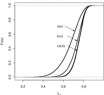
The test statistics use the entropy estimators and there is no criteria to select the optimal window size associated with a given sample size in order to calculate these estimators. As a guide mentioned by some authors, the window size producing the largest critical value for a givenn is apt to yield the highest power. In this sense, the optimal window size, denoted bym∗, at the significance level 0.1 for sample sizes 10, 20 and 30 are approximately 3, 3 and 4, respectively. Figure 1 shows a comparison of

CDF of the test statistics in differen designs. It is observed that the null distribution of

T3,10under SRS (RSS) is stochastically smaller than that under RSS (DRSS) (a similar trend is observed for sample sizesn=20,30). Thus, we expect the entropy test based on RSS (DRSS) to be more powerful than that based on SRS (RSS).

3. Simulation results

A Monte Carlo simulation experiment is carried out to compare power of the entropy tests. We considered three classes of alternatives presented by Stephens (1974) which have been used by many authors. These alternatives specified by their distribution functions are A(k):F(z) =1−(1−z)k _0≤ z≤1 (k=1.5,1.75,2), B(k):F(z) = 2k−1_zk 1−2k−1_(1−z)k 0≤z≤0.5 0.5≤z≤1 (k=1.5,1.75), and C(k):F(z) = 0.5−2k−1_(0.5−z)k 0.5+2k−1_(z−0.5)k 0≤z≤0.5 0.5≤z≤1 (k=2,2.5).

As compared with uniform, the first and second family give points closer to 0 and 0.5, respectively. And the third family gives points clustered at 0 and 1. We also considered Beta(2,2) as a symmetric distribution.

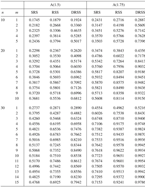
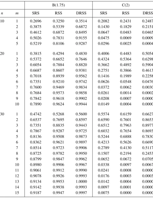
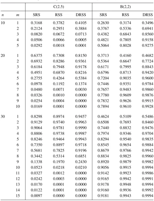
Under each design, 10,000 samples of sizesn=10,20,30 were generated from each alternative distribution and the power of the tests were estimated by proportion of the samples falling into the corresponding critical region. Tables 3–6 exhibit the estimated power of the tests.

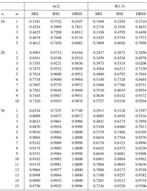
The results manifest that given a sample size, the entropy tests based on RSS and DRSS are more powerful than that based on SRS irrespective of the alternative distribution. Moreover, improved tests are obtained by increasing the sampling effort. That is DRSS has the best performance among three considered designs as is the case of entropy estimation. This could be traced to the fact that the test statistic in each design is constructed based on the corresponding entropy estimator. It is notable that RSS and DRSS do not have much to offer when power of SRS design is less than 0.1. We observe that forn=10, the valuem=4 is best (in the sense that it yields the highest power) for the tests under most alternatives except C (for whichm=1 is best). For n=20, bestmfor alternatives A, B and C are respectively 7, 10 and 2, while for n=30 these are 10, 15 and 3. Given a sample size, bestmis different according to the alternative

Table 3: Power comparison for the entropy tests of size 0.1 against alternatives A(1.5) and A(1.75).

A(1.5) A(1.75) n m SRS RSS DRSS SRS RSS DRSS 10 1 0.1745 0.1879 0.1924 0.2431 0.2716 0.2887 2 0.2182 0.2668 0.3360 0.3147 0.4198 0.5609 3 0.2325 0.3306 0.4635 0.3451 0.5276 0.7142 4 0.2397 0.3814 0.5285 0.3570 0.5766 0.7628 5 0.2436 0.3794 0.5017 0.3503 0.5728 0.7396 20 1 0.2298 0.2367 0.2620 0.3474 0.3843 0.4356 2 0.3052 0.3530 0.4098 0.4786 0.6022 0.7178 3 0.3292 0.4351 0.5174 0.5342 0.7264 0.8413 4 0.3704 0.5064 0.6030 0.5760 0.7956 0.9032 5 0.3728 0.5301 0.6386 0.5817 0.8207 0.9186 6 0.3846 0.5693 0.6962 0.5932 0.8494 0.9451 7 0.3817 0.5867 0.7092 0.5870 0.8575 0.9482 8 0.3754 0.5801 0.7126 0.5821 0.8490 0.9436 9 0.3720 0.5718 0.6996 0.5713 0.8358 0.9322 10 0.3681 0.5536 0.6812 0.5608 0.8114 0.9156 30 1 0.2737 0.2871 0.2890 0.4554 0.4962 0.5216 2 0.3795 0.4287 0.4882 0.6026 0.7538 0.8430 3 0.4260 0.5468 0.6324 0.6748 0.8710 0.9406 4 0.4556 0.6195 0.6958 0.7106 0.9175 0.9748 5 0.4821 0.6536 0.7476 0.7382 0.9387 0.9824 6 0.4926 0.6783 0.7662 0.7512 0.9435 0.9870 7 0.5016 0.6985 0.8210 0.7533 0.9516 0.9936 8 0.5137 0.7245 0.8344 0.7642 0.9578 0.9945 9 0.5068 0.7352 0.8490 0.7618 0.9622 0.9934 10 0.5184 0.7510 0.8538 0.7723 0.9651 0.9927 11 0.5170 0.7486 0.8612 0.7674 0.9601 0.9954 12 0.4996 0.7442 0.8569 0.7505 0.9570 0.9932 13 0.4954 0.7355 0.8556 0.7410 0.9513 0.9942 14 0.4825 0.7190 0.8230 0.7295 0.9372 0.9900 15 0.4768 0.6925 0.7942 0.7153 0.9241 0.9786

Table 4: Power comparison for the entropy tests of size 0.1 against alternatives A(2) and B(1.5).

A(2) B(1.5) n m SRS RSS DRSS SRS RSS DRSS 10 1 0.3181 0.3742 0.4107 0.1948 0.2245 0.2310 2 0.4254 0.5969 0.7821 0.2716 0.3520 0.4633 3 0.4635 0.7208 0.8913 0.3188 0.4795 0.6490 4 0.4674 0.7648 0.9134 0.3425 0.5734 0.7572 5 0.4612 0.7430 0.8882 0.3609 0.6026 0.7698 20 1 0.4983 0.5712 0.6344 0.2417 0.2672 0.2856 2 0.6541 0.8348 0.9318 0.3458 0.4236 0.4978 3 0.7103 0.9221 0.9830 0.3973 0.5324 0.6206 4 0.7472 0.9532 0.9926 0.4564 0.6213 0.7230 5 0.7624 0.9608 0.9952 0.4900 0.6792 0.7844 6 0.7718 0.9680 0.9964 0.5140 0.7328 0.8465 7 0.7697 0.9735 0.9972 0.5406 0.7760 0.8751 8 0.7562 0.9658 0.9948 0.5510 0.8035 0.8924 9 0.7445 0.9567 0.9931 0.5636 0.8142 0.9172 10 0.7320 0.9453 0.9876 0.5727 0.8210 0.9204 30 1 0.6324 0.7255 0.7740 0.2911 0.3128 0.3397 2 0.8009 0.9472 0.9872 0.4085 0.4939 0.5516 3 0.8613 0.9861 0.9986 0.4821 0.6174 0.7050 4 0.8870 0.9934 0.9998 0.5349 0.6960 0.7812 5 0.9010 0.9963 1.0000 0.5719 0.7486 0.8305 6 0.9084 0.9968 1.0000 0.6034 0.7764 0.8570 7 0.9142 0.9980 0.9998 0.6170 0.8123 0.8996 8 0.9175 0.9985 1.0000 0.6452 0.8375 0.9230 9 0.9151 0.9984 0.9998 0.6636 0.8681 0.9408 10 0.9182 0.9992 1.0000 0.6901 0.8894 0.9562 11 0.9135 0.9981 1.0000 0.7004 0.9045 0.9636 12 0.9064 0.9977 1.0000 0.7088 0.9173 0.9748 13 0.8998 0.9964 1.0000 0.7190 0.9257 0.9782 14 0.8890 0.9932 1.0000 0.7201 0.9212 0.9718 15 0.8756 0.9925 0.9996 0.7236 0.9220 0.9706

Table 5: Power comparison for the entropy tests of size 0.1 against alternatives B(1.75) and C(2).

B(1.75) C(2) n m SRS RSS DRSS SRS RSS DRSS 10 1 0.2696 0.3250 0.3514 0.2082 0.2431 0.2487 2 0.3875 0.5339 0.6872 0.1430 0.1829 0.2151 3 0.4612 0.6872 0.8495 0.0647 0.0483 0.0465 4 0.5026 0.7831 0.9155 0.0475 0.0069 0.0009 5 0.5219 0.8106 0.9287 0.0296 0.0025 0.0004 20 1 0.3815 0.4294 0.4830 0.4006 0.4483 0.5054 2 0.5372 0.6652 0.7646 0.4324 0.5364 0.6298 3 0.6054 0.7884 0.8820 0.3662 0.4892 0.5904 4 0.6687 0.8607 0.9381 0.2751 0.3866 0.4613 5 0.7018 0.8939 0.9562 0.1416 0.1989 0.2258 6 0.7351 0.9210 0.9742 0.0626 0.0548 0.0476 7 0.7600 0.9469 0.9834 0.0372 0.0062 0.0030 8 0.7684 0.9573 0.9858 0.0261 0.0014 0.0002 9 0.7842 0.9618 0.9902 0.0208 0.0007 0.0000 10 0.7890 0.9624 0.9944 0.0149 0.0004 0.0000 30 1 0.4742 0.5268 0.5600 0.5574 0.6159 0.6627 2 0.6537 0.7695 0.8597 0.6590 0.7601 0.8653 3 0.7351 0.8835 0.9443 0.6512 0.7963 0.8977 4 0.7867 0.9287 0.9725 0.6032 0.7654 0.8693 5 0.8136 0.9508 0.9873 0.5244 0.6888 0.7830 6 0.8362 0.9621 0.9897 0.4213 0.5626 0.6690 7 0.8514 0.9723 0.9906 0.2789 0.4130 0.5117 8 0.8725 0.9782 0.9950 0.1507 0.2194 0.2453 9 0.8799 0.9847 0.9962 0.0652 0.0672 0.0705 10 0.8980 0.9906 0.9967 0.0338 0.0097 0.0067 11 0.9061 0.9912 0.9990 0.0241 0.0008 0.0000 12 0.9078 0.9926 0.9993 0.0176 0.0003 0.0003 13 0.9134 0.9953 1.0000 0.0142 0.0004 0.0000 14 0.9142 0.9938 0.9993 0.0097 0.0001 0.0000 15 0.9187 0.9947 0.9997 0.0075 0.0000 0.0000

Table 6: Power comparison for the entropy tests of size 0.1 against alternatives C(2.5) and B(2,2).

C(2.5) B(2,2) n m SRS RSS DRSS SRS RSS DRSS 10 1 0.3168 0.3782 0.4105 0.2630 0.3174 0.3496 2 0.2124 0.2951 0.3884 0.3767 0.5336 0.6941 3 0.0820 0.0672 0.0713 0.4382 0.6843 0.8560 4 0.0506 0.0066 0.0005 0.4821 0.7805 0.9158 5 0.0292 0.0018 0.0001 0.5064 0.8028 0.9275 20 1 0.6375 0.7308 0.8150 0.3713 0.4160 0.4682 2 0.6932 0.8286 0.9361 0.5364 0.6647 0.7724 3 0.6184 0.7948 0.9178 0.6171 0.7995 0.8843 4 0.4951 0.6870 0.8216 0.6796 0.8713 0.9420 5 0.2755 0.4264 0.5384 0.7204 0.9035 0.9600 6 0.0978 0.1192 0.1374 0.7446 0.9351 0.9784 7 0.0480 0.0071 0.0030 0.7657 0.9483 0.9860 8 0.0326 0.0010 0.0000 0.7780 0.9609 0.9876 9 0.0254 0.0004 0.0000 0.7832 0.9626 0.9915 10 0.0169 0.0001 0.0000 0.7894 0.9610 0.9928 30 1 0.8298 0.8974 0.9457 0.4624 0.5109 0.5486 2 0.9129 0.9740 0.9963 0.6508 0.7693 0.8460 3 0.9064 0.9781 0.9990 0.7440 0.8832 0.9476 4 0.8806 0.9738 0.9987 0.7974 0.9346 0.9704 5 0.8246 0.9464 0.9943 0.8294 0.9540 0.9835 6 0.7350 0.8897 0.9718 0.8545 0.9654 0.9884 7 0.5681 0.7825 0.9196 0.8679 0.9766 0.9942 8 0.3442 0.5314 0.6851 0.8834 0.9825 0.9960 9 0.1338 0.1970 0.2430 0.8920 0.9879 0.9982 10 0.0523 0.0218 0.0210 0.9056 0.9915 0.9994 11 0.0327 0.0012 0.0000 0.9142 0.9923 0.9986 12 0.0242 0.0003 0.0000 0.9165 0.9942 0.9991 13 0.0170 0.0001 0.0000 0.9178 0.9948 0.9994 14 0.0122 0.0001 0.0000 0.9160 0.9936 0.9992 15 0.0097 0.0000 0.0000 0.9181 0.9943 0.9994

distribution. As a remedy, we may use data histogram to determine best window size for implementing the tests. Table 7 compares the power of RSS entropy based test for uniformity, whenmis best, with that of the KS test whose results are given in italic. It is seen that entropy test shows remarkable dominance over the KS test against alternatives B and B(2,2), whereas the KS test is better for alternatives A and C.

Table 7: Power comparison for the entropy test and KS test of size 0.1 against several alternative distributions under RSS.

Distribution

n A(1.5) A(1.75) A(2) B(1.5) B(1.75) C(2) C(2.5) B(2,2)

10 0.381 0.577 0.765 0.603 0.811 0.243 0.378 0.803 0.629 0.875 0.971 0.176 0.290 0.583 0.798 0.235 20 0.587 0.858 0.974 0.821 0.962 0.536 0.829 0.961 0.884 0.993 1.000 0.327 0.566 0.845 0.975 0.482 30 0.751 0.965 0.999 0.922 0.995 0.796 0.978 0.994 0.970 1.000 1.000 0.463 0.768 0.950 0.997 0.691

Table 8: 0.1 critical points of the test statistics under MSRSS designs. Stage Number

n(m∗_{) r=2 r=3 r=4}

10(3) 0.6725 0.6910 0.7048

20(3) 0.7706 0.7892 0.7956

30(4) 0.8143 0.8236 0.8281

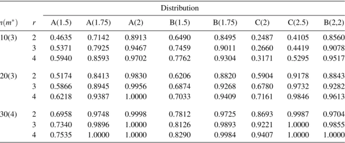
Table 9: Power comparison for the entropy tests of size 0.1 against several alternative distributions under MSRSS designs.

Distribution

n(m∗_{) r A(1.5) A(1.75) A(2) B(1.5) B(1.75) C(2) C(2.5) B(2,2)}

10(3) 2 0.4635 0.7142 0.8913 0.6490 0.8495 0.2487 0.4105 0.8560 3 0.5371 0.7925 0.9467 0.7459 0.9011 0.2660 0.4419 0.9078 4 0.5940 0.8593 0.9702 0.7762 0.9304 0.3171 0.5295 0.9517 20(3) 2 0.5174 0.8413 0.9830 0.6206 0.8820 0.5904 0.9178 0.8843 3 0.5866 0.8945 0.9956 0.6874 0.9268 0.6780 0.9732 0.9282 4 0.6218 0.9387 1.0000 0.7033 0.9409 0.7161 0.9846 0.9613 30(4) 2 0.6958 0.9748 0.9998 0.7812 0.9725 0.8693 0.9987 0.9704 3 0.7340 0.9896 1.0000 0.8126 0.9893 0.9221 1.0000 0.9855 4 0.7535 1.0000 1.0000 0.8290 0.9984 0.9407 1.0000 1.0000

Tables 2 and 3–6 were formed under MSRSS withr=3,4 to see whether further increase in power is achieved by increasing the stage number. Tables 8 and 9 contain 0.1 critical points and power of the tests, respectively. For a givenn, the results are provided only for the optimalm, except forCfamily and n=10 wherem=1 is applied. Also, results of DRSS design were included to ease comparison. From Table 9, we can see that asrincreases, some improvement in power happens. The differences in results for

r=2 andr=3,4 are less pronounced in large sample size, and thus we may restrict ourselves to DRSS in practice.

4. Conclusion

This article was directed at the problem of developing tests of uniformity under RSS and MSRSS designs. In line with the available entropy based test of fit in SRS, our tests use sample entropy based on the pre-mentioned designs. Simulation studies accompany the presentation to explore power behaviour of the proposed tests in finite sample sizes. The results disclose that RSS and its variations outperform SRS in constructing powerful entropy based test of uniformity. The authors have developed similar tests for other distributions (e.g. uniform, beta, exponential, gamma, log-normal, Pareto, Rayleigh, Weibull, normal, Laplace, etc.) using improved entropy estimators (e.g., see Ebrahimi et al. (1994) and Novi Inverardi (2003)). The results will be reported in separate works.

Acknowledgements

The authors are grateful to the referees for their helpful comments that clearly improved this article. Partial support from “Ordered and Spatial Data Center of Excellence of Ferdowsi University of Mashhad” is acknowledged.

References

Adatia, A. (2003). Estimation of parameters of uniform distribution using generalized ranked set sampling. Journal of Statistical Research, 37, 193–202.

Adatia, A. and Ehsanes Saleh, A. K. Md. (2004). Estimation of quantiles of uniform distribution using

generalized ranked-set sampling.Pakistan Journal of Statistics, 20, 355–368.

Al-Saleh, M. F. and Al-Kadiri, M. (2000). Double ranked set sampling.Statistics & Probability Letters, 48,

205–212.

Al-Saleh, M. F. and Al-Omari, A. I. (2002). Multistage ranked set sampling.Journal of Statistical Planning

and Inference, 102, 273–286.

Ash, R. B. (1965).Information Theory. John Wiley & Sons, New York.

Chen, Z., Bai, Z. and Sinha, B. K. (2004).Ranked set sampling: Theory and Applications. Springer, New

York.

Dudewicz, E. J. and van der Meulen, E. C. (1981). Entropy-based tests of uniformity.Journal of the Amer-ican Statistical Association, 76, 967–974.

Ebrahimi, N., Pflughoeft, K. and Soofi, E. S. (1994). Two measures of sample entropy.Statistics &

Proba-bility Letters, 20, 225–234.

Gokhale, D. V. (1983). On the entropy-based goodness-of-fit tests. Computational Statistics and Data

Analysis, 1, 157–165.

Grzegorzewski, P. and Wieczorkowski, R. (1999). Entropy based goodness-of-fit test for exponentiality. Communications in Statistics–Theory and Methods, 28, 1183–1202.

Gulati, S. (2004). Smooth non-parametric estimation of the distribution function from balanced ranked set

samples.Environmetrics, 15, 529–539.

Mahdizadeh, M. and Arghami, N. R. (2010). Efficiency of ranked set sampling in entropy estimation and

goodness-of-fit testing for the inverse Gaussian law.Journal of Statistical Computation and

Simula-tion, 80, 761–774.

McIntyre, G. A. (1952). A method of unbiased selective sampling using ranked sets.Australian Journal of

Agricultural Research, 3, 385–390.

Mudholkar, G. S. and Tian, L. (2002). An entropy characterization of the inverse Gaussian distribution and

related goodness-of-fit test.Journal of Statistical Planning and Inference, 102, 211–221.

Novi Inverardi, P. L. (2003). MSE comparison of some different estimators of entropy.Communications in

Statistics–Simulation and Computation, 32, 17–30.

Stokes, S. L. and Sager, T.W. (1988). Characterization of a ranked-set sample with application to estimating

distribution function.Journal of the American Statistical Association, 83, 374–381.

Shannon, C. E. (1948). A mathematical theory of communications.Bell System Technical Journal, 27, 379–

423, 623–656.

Stephens, M. A. (1974). EDF statistics for goodness of fit and some comparisons.Journal of the American

Statistical Association, 69, 730–737.

Vasicek, O. (1976). A test of normality based on sample entropy.Journal of the Royal Statistical Society: