McCreesh, N; Frost, SD; Seeley, J; Katongole, J; Tarsh, MN; Ndun-guse, R; Jichi, F; Lunel, NL; Maher, D; Johnston, LG; Sonnenberg, P; Copas, AJ; Hayes, RJ; White, RG (2012) Evaluation of Respondent-driven Sampling. Epidemiology (Cambridge, Mass), 23 (1). pp. 138-147. ISSN 1044-3983 DOI: https://doi.org/10.1097/EDE.0b013e31823ac17c
Downloaded from: http://researchonline.lshtm.ac.uk/28547/ DOI:10.1097/EDE.0b013e31823ac17c
Usage Guidelines
Please refer to usage guidelines at http://researchonline.lshtm.ac.uk/policies.html or alterna-tively [email protected].
Evaluation of Respondent-Driven Sampling
Original Article
Authors
McCreesh, Nicky1, Frost, Simon2, Seeley, Janet3,4, Katongole, Joseph3, Ndagire Tarsh.
Matilda3, Ndungutse, Richard3, Jichi. Fatima1, Tilson, Natasha1, Maher, Dermot3, Sonnenberg, Pam5, Copas, Andrew5, Hayes, Richard J1, White, Richard G1
Corresponding author
Dr Richard White, Department of Infectious Disease Epidemiology, Faculty of Epidemiology & Population Health, London School of Hygiene and Tropical Medicine, Keppel Street, London WC1E 7HT. Tel: + 44 (0) 20 7299 4626 Email: [email protected]
Keywords: Respondent-Driven Sampling, RDS,Uganda, HIV, sexual behaviour, socioeconomic status, statistical inference, method
Sources of financial support
RGW is funded by a Medical Research Council (UK) Methodology Research Fellowship (G0802414), the Gates Foundation (19790.01), and the EU FP7 (242061). SDWF is funded by the National Institutes of Nursing Research (grant NR10961), the National Institute on Drug Abuse (grant DA24998), and by a Royal Society Wolfson Research Merit Award. The general population cohort in Uganda is funded by the Medical Research Council (UK). The funders had no involvement in the design, collection, analysis or interpretation of the data, in writing the report or in the decision to submit.
Acknowledgements
The authors would particularly like thank the study participants and staff at the MRC/UVRI Uganda Research Unit on AIDS, without whom this study would not have been possible.
1Department of Infectious Disease Epidemiology, Faculty of Epidemiology & Population Health,
London School of Hygiene and Tropical Medicine, UK
2 Department of Veterinary Medicine, University of Cambridge. UK
3 MRC/UVRI Uganda Research Unit on AIDS, Entebbe, Uganda
4 School of International Development, University of East Anglia, Norwich, UK
5 Department of Infection and Population Health, University College London, UK
Background
Respondent-driven sampling(RDS) is a novel variant of snowball sampling for estimating the characteristics of hard-to-reach groups, such as HIV prevalence in sex-workers. Despite use by leading heath organisations, the performance of RDS in realistic situations is still largely unknown. This study evaluated RDS by comparing estimates from an RDS survey with total-population data.
Methods
Total-population data on age, tribe, religion, socioeconomic status, sexual activity and HIV status were available on a population of 2402 male household-heads from an open cohort in rural Uganda. An RDS survey was carried out in this population, employing current RDS methods of sampling(RDS-sample) and statistical inference(RDS-estimates). Analyses were repeated for the full RDS sample and the first 250 recruits(small sample).
Results
927 household-heads were recruited. Full and small RDS-samples were largely
representative of the total population, but under-represented men who were younger, of higher socioeconomic status, and with unknown sexual activity and HIV status. RDS statistical inference methods failed to reduce these biases. Only 31-37%(depending on method and sample size) of RDS-estimates were closer to the true population proportions than the RDS-sample proportions. Only 50-74% of RDS bootstrap 95% CIs included the population proportion.
Conclusions
RDS produced a generally representative sample of this well-connected non-hidden
population. However, current RDS inference methods failed to reduce bias when it occurred. Whether the data required to remove bias and measure precision can be collected in an RDS survey is unresolved. RDS should be regarded as a(potentially superior) form of convenience sampling method, and caution is required when interpreting RDS findings.
Introduction
Hidden or hard-to-reach population subgroups are often key to the maintenance of infectious
diseases in human populations.1 But, it is often difficult to investigate the factors that drive
transmission in these groups using representative samples because there may not be an adequate sampling frame or the groups may be associated with illicit activity or subject to stigma. Therefore researchers have typically resorted to various types of convenience sampling to gather data on hidden populations.2 While convenience sampling has its
advantages, it is unable to generate unbiased population-based estimates of infection prevalence and risk factors.
In an attempt to address these limitations, a type of snowball sampling, respondent-driven sampling was proposed in 1997.3 First, a small number of seeds are selected by
convenience or other methods. Then, these initial recruits are given coupons, typically 3, to recruit others from the target population, who themselves become recruiters. Recruits are given an incentive, usually money, for taking part in the survey and also for recruiting others. This process continues in recruitment ‘waves’until a pre-determined sample size is reached or the distribution of participant characteristics (such as the proportion infected) becomes similar between waves (called reaching ‘equilibrium’ in respondent-driven sampling
terminology). Estimation methods are then applied to account for the non-random sample selection in an attempt to generate unbiased estimates for the target population. To enable the sample to be collected, the target population must be socially well-connected.
Two main estimation methods are used The ‘RDS-1’ estimator is currently in wide use and is implemented in the standard respondent-driven sampling analysis software.3-6 RDS-1
accounts for patterns of recruitment between subgroups and the average number of other members of the target group recruiters know (the ‘network size’) in each subgroup.5,7
‘RDS-2’ is a more recently developed estimator that relates respondent-driven sampling estimation to widely used survey estimation through the use of a generalized Horvitz-Thompson
estimator.8 RDS-2 accounts for network size only.8 Initial theoretical analysis has asserted
that the RDS-2 estimator is asymptotically unbiased as long as six key assumptions are met, including that respondents accurately report the size of their ‘network’ (the number of other members of the target group they know), respondents randomly recruit from their network, and respondents have reciprocal relationships with members of the target population8
A recent study simulating respondent-driven sampling and using empirical network data found that the variance of respondent-driven sampling estimates can be much higher than commonly assumed.9 Nevertheless, respondent-driven sampling has rapidly become a
popular and widely used survey method. Outside of the US, over 123 respondent-driven sampling studies have been published that collectively recruited over 30,000 individuals10
and respondent-driven sampling is currently being employed to provide data for public health decision making by major funding bodies such as the US Centre for Disease Control and Prevention.
Despite this rapid increase in popularity and use by major funding bodies, whether respondent-driven sampling could generate unbiased estimates is largely unknown. This is primarily because the robust evaluation of respondent-driven sampling is methodologically challenging. By definition, the ‘gold-standard’ representative or total-population data that are required, are generally unavailable or are of poor quality for hidden/stigmatised groups. As such other methods of evaluation have been attempted including in-silico studies,4,8,11-12
comparing respondent-driven sampling data to data from other convenience samples,13-19
comparing cross-sectional respondent-driven sampling estimates on the same population over time20 and comparing internet-collected respondent-driven sampling data to a
population with known characteristics.21-22 Although all these studies have provided valuable
information on respondent-driven sampling, none provide a robust assessment of whether respondent-driven sampling could produce unbiased estimates, because the required ‘gold-standard’ comparison population was unavailable or an internet-based respondent-driven
sampling data collection method was used, whereas the vast majority of respondent-driven sampling studies employ a face-to-face method to collect field data.10
We present the first study to evaluate respondent-driven sampling by comparing field-collected respondent-driven sampling data with total population data on the same population. We dealt with the problem that the representative or total-population data that are required for this comparison are generally unavailable, by evaluating respondent-driven sampling in a non-hidden/non-stigmatised population on which high quality total population data were available. This also allowed us to perform a range of analyses that are not possible in typical respondent-driven sampling studies.
Methods
The aim of this study was to evaluate whether respondent-driven sampling could generate representative data on a rural Ugandan population by comparing estimates from an
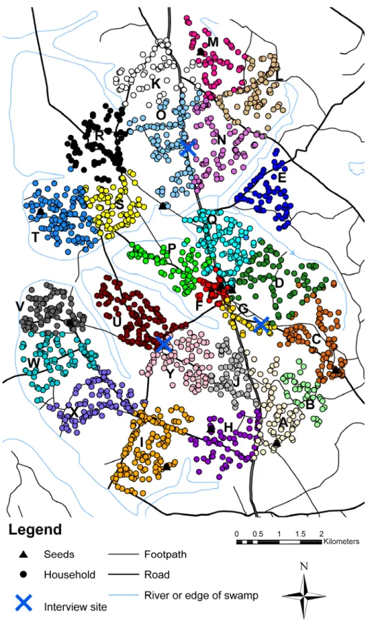
respondent-driven sampling survey with total-population data. The data used to define the target population were available from an ongoing general population cohort of 25 villages in rural Uganda covering an area of approximately 38km23-24 (Figure 1). Each year, households
in the study villages are mapped and after obtaining consent, a total-population household census and an individual questionnaire and HIV-1 serosurvey are administered. The target population consisted of 2402 men who were recorded as a male head of a household within these villages between February 2009 and January 2010 (Figure 1). The characteristics of the target population are shown in Table 1 (population proportion).
To maximise the generalisability of our results, where possible we employed currently used respondent-driven sampling data collection methods.10 Ten seeds (of varying village, age
and tribe) were selected by convenience from the target population. Figure 1 shows their locations and Table S1 summarises their characteristics. Seeds and subsequent recruits were given three coupons to recruit other men into the study. The rate of early recruitment was high and the number of people arriving each day for interviews became too large. Because of this, between day nine and 32 the probability of each recruit being offered three coupons was halved from 100% to 50% and other recruits received none. Seeds and recruits were offered incentives for participation and recruitment, either soap, salt or school books to the value of ~$1US. One incentive was offered for completing the first interview and another for each person successfully recruited.
Respondent-driven sampling estimation requires information on how many other household heads each participant could potentially recruit. The primary network size definition (NS1) was created to be comparable with other respondent-driven sampling studies25-26 and was
used in this paper unless otherwise stated. Recruits were first asked the core question “How
many men do you know who (i) were head of a household in the last 12 months in any of the Medical Research Council villages, and (ii) you know them and they know you, and (iii) you have seen them in the past week”. More detailed network data were also collected (see
supporting methods).
Pre-processing of the data was performed using Stata v11 (StataCorp, Texas).27 Networks
and trees were generated using scripts written in Stata and R v2.12.0 (R Foundation,
Vienna)28 and visualized using GraphViz (AT&T Research, New Jersey).29 To maximise the
comparability of our methods with those used in a typical respondent-driven sampling study, we analysed the dataset following current respondent-driven sampling definitions and the statistical inference methods employed in RDSATv6.0.1, the custom written software package for the analysis of respondent-driven sampling studies.6 (ie the ‘RDS-1’ point
estimator3-5 and the bootstrap 95% interval estimator11). We also analysed the dataset using
the more recently developed point estimator ‘RDS-2’ and the same bootstrap 95% interval estimator,11 employing R. Simple respondent-driven sampling sample proportions and
respondent-driven sampling estimates were calculated for two different sample sizes. The first was the ‘Full’ sample (n=927 including the 10 seeds). The second was a ‘Small’ sample consisting of the first 250 recruits (including the 10 seeds) and was chosen to be more typical of the sample sizes used in respondent-driven sampling studies.10
Root mean squared errors were calculated for the difference between the population proportions and the full and small sample proportions, and for the difference between the population proportions and the RDS-1 and RDS-2 estimates, for each variable and in total. For comparison with the RDS-1 and RDS-2 estimates, we used the true population
proportions to calculate recruitment probabilities for the target population using predictions from a logistic regression model30 as weights. The variables shown in Table 1 were included
in the model if they were significant at the 95% confidence level.
Sensitivity analyses were used to assess the robustness of our results to different network size definitions, potential network size bias and respondent-driven sampling sample size.
To compare network size of the whole target population to the respondent-driven sampling recruits, 300 men in the target population who had not been recruited in the respondent-driven sampling study were selected using simple random sampling to be interviewed using the first respondent-driven sampling questionnaire. Mean network size of the whole target population was estimated as the weighted average of the mean network size of RDS recruits and the mean network size of a simple random sample of eligible non-recruits. T-tests were used to test for difference between means. To help understand the quantitative study findings, 54 members of the population in the study villages or Medical Research Council staff were selected using random or purposive sampling for qualitative interview. Full details are shown in supporting methods.
Results Recruitment
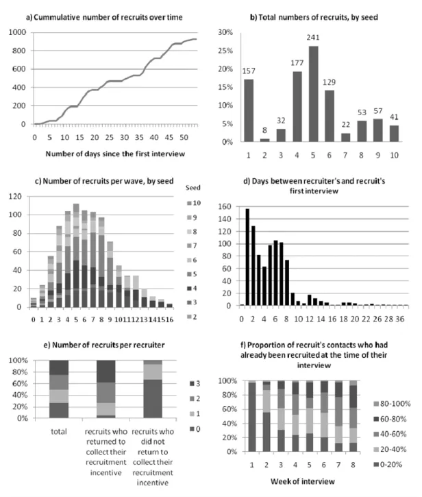
The dynamics of the respondent-driven sampling survey recruitment is shown in Figure 2 and the recruitment networks from each seed are shown in Figure 3. A total of 1141 people (including the 10 seeds) were assessed for eligibility over a period of 54 days (8th March – 30th April 2010) (Figure 2a). No new coupons were distributed after day 47. 196 men attended but were ineligible, 16 were eligible but had already been recruited, 2 were eligible but did not give consent, and 927 were eligible, consented and were recruited. A video illustrating recruitment in space and time is shown in the supporting results. A roughly linear recruitment rate was achieved in the respondent-driven sampling survey (Figure 2a), due, in part, to changes in the probability of each recruit being offered coupons during the survey. All 10 seeds recruited people into the study, with one seed recruiting one person, four recruiting two people, and five recruiting three people. The total number of recruits
originating from each seed ranged from 8 to 241 (1% to 26% of the full sample) (Figure 2b). 77% of the total recruitment was from four seeds. Full details of the seeds and recruitment by seed are given in supporting Table S1. The number of waves ranged from 3 to 16 for the full sample and 2 to 6 for the small sample Most recruitment occurred in wave five (12% of all recruits, excluding seeds) and 57% of recruitment occurred in waves four to eight (Figure 2c). 81% of recruits (including the recruits of seeds) were interviewed within 7 days of their recruiter’s interview (Figure 2d).
Overall, 75% of recruits (including seeds) (684) were offered coupons to recruit others, and of these 90% (612) accepted (called ‘recruiters’). 66% of recruiters (401) returned for a second interview and to collect their secondary incentives. A similar proportion of recruiters (including seeds) recruited zero, one, two and three recruits (Figure 2e, left bar). Recruits who returned to collect secondary incentives were more likely to have recruited (Figure 2e, middle and right bar). The proportion of the recruit’s network who had already been recruited at the time of their interview increased rapidly during the survey (Figure 2f, includes seeds).
The average number of recruits per recruiter (including seeds) decreased from 2.57 in the first week of the study to 0.62 in the last week that coupons were given out. Only 30% of recruits were given as a contact by their recruiter (and identified) at their recruiter’s first interview,
In the simple random sample survey, 55% (164/300) of the men selected were interviewed (4th - 28th May 2010; supporting results ‘simple random sample survey’). In the qualitative
survey, 98% of (53/54) people selected were interviewed (16th June - 19th Oct 2010;
supporting results ‘Qualitative survey’).
The target population was well-connected. Data from the respondent-driven sampling and simple random sampling surveys showed that at least 73% were linked in a single network (see supporting methods). The distribution of the reported network size (NS1) of
respondent-driven sampling recruits was approximately Normal but with a slight positive skew, and shows likely over-reporting of multiples of 5 (supporting Figure S1, excluding seeds). The distributions of the other network size measures were very similar, with the exception of definition NS5, which, by definition, showed a smaller proportion of larger network sizes, because it was a subset of NS4 (supporting Figure S2, including seeds). Pearson correlations between different network size definitions reported by respondent-driven sampling recruits varied between 0.96 (NS1 vs NS2) and 0.75 (NS1 vs. NS5)
(supporting Table S2, including seeds). The mean network size (NS1) of respondent-driven sampling recruits (including seeds) was higher than that of the whole target population(12.1 vs 9.2, p<0.001) (supporting Figure S3). The number of times members of the target population were reported to be in the network of recruits ranged between 0 and 42 (supporting Figure S4).
There were high levels of homophily indicating high within-group recruitment by religion, tribe, village and in the highest socioeconomic status group, but not by age, the other
socioeconomic status groups, sexual activity or HIV status (supporting Table S3 and Table S4). There was no evidence of low within-group recruitment for any characteristic, i.e. preferentially recruiting men who differed from themselves. Comparing actual recruitment proportions with expected recruitment proportions calculated from individual level network data, there was evidence of non-random recruitment by age, tribe, socioeconomic status, village and sexual activity (supporting results ‘Recruitment pattern’ section and supporting tables S5 and S6).
The other RDS2 estimator assumptions8 were not met. In common with current practice for
all RDS studies, respondents were not limited to recruiting only one other individual and recruited individuals were ineligible for re-recruitment. It is likely that a low proportion of the relationships between members of the target population were reciprocated and/or the population may not have accurately reported their network size as only 30% of recruits were mentioned by their recruiter during the recruiter’s first interview.
Comparison with target population data
Table 1 shows the comparison between the population proportions, sample proportions, and RDS-1 and RDS-2 estimates with 95% CIs, for the full and small sample. The sample proportions were often similar to population proportions, with the following exceptions. In both samples, younger men (<30 years) were underrepresented and older men (≥40 years) were overrepresented. In the small sample, Catholics were overrepresented. In both samples men in the highest socioeconomic group were underrepresented and men in the lowest socioeconomic group were overrepresented. The proportions of men with unknown number of sexual partners or unknown HIV status were underrepresented in both samples. Due to the size of the differences between the population and sample proportions for these groups, it is unlikely that they occurred by chance (p≤0.0001 for all except p=0.04 for the highest socio-economic status group using the small sample).
Respondent-driven sampling inference methods generally failed to reduce bias where it occurred. Adjustment resulted in an improved estimate of the population proportion in only 37% (19/52) of comparisons using RDS-1 and 33% (15/52) using RDS-2 for the full sample, and 31% (8/26) using RDS-1 and 37% (18/49) using RDS-2 for the small sample. Based on these estimates, the 95% bootstrap confidence intervals included the target population proportion in 69% (36/52) of comparisons using RDS-1 and 50% (13/26) using RDS-2 for the full sample, and 69% (18/26) using RDS-1 and 74% using RDS-2 for the small sample.
The root mean squared error for the difference between the population proportions and the sample proportions was 6% for the full sample. The root mean squared error for the
difference between the population proportions and the respondent-driven sampling estimates for the full sample were 7% for both RDS-1 and RDS-2 (supporting table S7). Root mean squared errors were slightly larger for the small sample.
In general the respondent-driven sampling adjustments that did not improve the estimates were small, and therefore did not add substantial bias. The exception to this was village. Due to the large number of subgroups for village, however, the sample size was not sufficiently large to reliably estimate the parameters used in making RDS-1 adjustments.
By comparison, using the predictions from the logistic regression as recruitment probability weights, adjustment resulted in an improved estimate of the target population proportion for 87% (45/52) of the full sample estimates, and 59% (29/49) of the small sample estimates (supporting Table S6), showing recruitment was associated with characteristics other than network size.
For those specific cases where the sample estimates were biased estimates of the population proportions, current respondent-driven sampling inference methods generally failed to reduce bias. For age group, using either the RDS-1 or the RDS-2 estimator only 2/5
estimates were closer to the population proportion when applied to the full sample, and only 1/4 when applied to the small sample. Neither RDS-1 nor RDS-2 improved the
over-representation of Catholics in the small sample; the over-over-representation of the lowest socioeconomic group in the full sample; the under-representation of the highest
socioeconomic group in either sample; or the underrepresentation of men with unknown number of sexual partners in either sample. Applying RDS-2 to the full sample very slightly reduced the under-representation of men with unknown HIV status. Applying RDS-2 to the small sample or RDS-1 to either sample slightly increased the under-representation of men with unknown HIV status.
Respondent-driven sampling inference methods failed to reduce bias because groups tended to be under or over-recruited by all groups, rather than being under-recruited by some groups and over-recruited by other groups (limiting the ability of RDS-1 to improve estimates), and under-represented groups tended not to have markedly smaller network sizes (limiting the ability of RDS-1 and RDS-2). For example, men aged 50+ years were over-recruited by all age groups and network sizes in all age groups were relatively similar (supporting Table S3). Therefore neither RDS-1 nor RDS-2 improved the estimates. Qualitative data suggested explanations for these findings. Recruiters did not consider younger unmarried men to be household heads in contrast with the definition used in the ongoing general population cohort
(“…they were being left out because some of the older men didn’t take them as household heads because they didn’t have any wives” [recruit, male, 45]). The respondent-driven
sampling incentives were likely to be a greater incentive to men in lower socioeconomic groups (“…the token might look small to some people and big to others." [community
member, female, 42]). The under-recruitment of men with unknown number of sexual partners or unknown HIV status was likely to be, at least in part, because men who had refused to participate in the ongoing general population cohort in the past were also less likely to participate in the respondent-driven sampling study.
There was very little difference in the performance of the respondent-driven sampling
estimators when different network size definitions were used (see supporting results). There was no evidence that collecting detailed network size data reduced the performance of the respondent-driven sampling estimators (see supporting results).
Discussion
The respondent-driven sampling method of recruitment produced a sample that was largely representative of the target population for most variables. The exceptions to this were an underrepresentation of younger men and men of higher socio-economic status, and an underrepresentation of men of unknown HIV status or unknown number of sexual partners in both samples, and an overrepresentation of Catholics in the small sample. The most
plausible reason for the bias in the sample with regards to age is that younger men were not considered to be heads of household. The most plausible reason for the bias in the sample with regards to socio-economic status is that men of higher socio-economic status were less attracted by the incentives given to recruits. Men who refused to participate in the ongoing general population cohort were probably more likely to also have refused to participate in respondent-driven sampling and that was probably at least partially responsible for the under-recruitment of men of unknown HIV status or with an unknown number of sexual partners. These biases may increase the design effect of respondent-driven sampling. Neither of the respondent-driven sampling inference methods was designed to correct for these sources of bias.
The bias in recruitment by socio-economic status is likely to be generalisable to most if not all respondent-driven sampling studies because different sub-groups of the target population are likely to be differentially incentivised by whatever (range of) incentives are offered. Although an ‘unknown’ category for HIV status and other variables will not exist in most other respondent-driven sampling studies, the differential recruitment of individuals in the
population by willingness to participate in surveys is likely to be a generalisable finding, but it is not limited to respondent-driven sampling. However, it is difficult to estimate the size of this bias using respondent-driven sampling data, as information on people who refuse to participate can only be obtained indirectly from the subset of recruiters who return to collect their secondary incentives. The bias in recruitment by age may not exist in other
driven sampling studies, but it does highlight another challenge for
driven sampling if the community understanding of target group membership does not (quite) correspond with the researcher’s definition. As in this case, the bias may be quite subtle and difficult to detect. Quantification of the size of the bias would require triangulation with other sources of quantitative data, and the explanation for the bias may only become clear if qualitative data are collected.
Overall, the sample proportions were closer to the population proportions than the respondent-driven sampling estimates more than 60% of the time, for both sample sizes. Both RDS-1 and RDS-2 adjustment slightly increased the total root mean squared error compared to the sample proportions. The overall failure of the respondent-driven sampling inference methods to reduce bias is likely to be due to the assumptions behind the
respondent-driven sampling method not being met, so that the methods imperfectly accounted for the patterns of recruitment between subgroups (RDS-1) and differences in network size (RDS-1 and RDS-2). Recruitment was associated with characteristics other than network size. The rather surprising finding that respondent-driven sampling inference methods increased bias more often than not was because, even when the respondent-driven sampling adjustments were in the right direction (eg. they reduced the size of estimate when the sample estimate was larger than the population proportion), the magnitude of the
adjustment was often more than twice the size of the bias, so that after adjustment the respondent-driven sampling estimate was further away from the population proportion.
The reason that the 95% confidence intervals included the population proportions substantially less than 95% of the time may be due either to the fact that the CIs are too narrow as has been suggested in another study,9 or because the respondent-driven sampling
estimates were biased, or a combination.
We have identified four primary potential limitations to our study. First, empirical evaluation of respondent-driven sampling is problematic. The representative or total-population data
that are required for robust evaluation are generally unavailable on the hidden and
stigmatised groups that respondent-driven sampling is most commonly used to survey. As such, we chose to evaluate respondent-driven sampling in a non-hidden/non-stigmatised population of male household heads, because of the availability of high quality
total-population data. This may limit the generalisability of our results. However it may also be a ‘best case scenario’ for an empirical evaluation of respondent-driven sampling. Respondent-driven sampling data on hidden and stigmatised populations may suffer from higher levels of bias than our sample. If respondent-driven sampling estimators are as unsuccessful at reducing this bias as our findings suggest, then estimates on hidden populations may be less representative than ours were. Second, the findings of this study are based on one
respondent-driven sampling sample only, and therefore the biases that we observed in the sample proportions could have arisen by chance. The differences between the population and sample proportions were highly unlikely to have occurred by chance however (p≤0.0001 for all differences except the under-representation of men in the highest socioeconomic group where p=0.04). In addition in each case where we identified a likely bias the qualitative data suggested a plausible reason why the bias occurred. Third, although we ordered the network size questions so that the first to be asked was similar to the question asked in most respondent-driven sampling studies,25-26 statements made by respondent-driven sampling
interviewers during the qualitative study suggested that the more detailed network questions may have caused later recuits to under-report network size so that the interview took less time. However, sensitivity analysis showed there was no evidence that collecting detailed network data reduced the performance of the respondent-driven sampling estimators and therefore we believe that our results and conclusions are robust to this potential limitation. Finally, our decision to not offer all recruits the chance to recruit others, to slow the rate of recruitment, could have biased the results. However, in general the respondent-driven sampling sample estimate was representative of the population proportions, and where the sample estimates were not, plausible explanations were identified for these biases. As such we believe that our results and conclusions are likely to be robust to this limitation.
In line with other studies respondent-driven sampling was demonstrated to be an effective data collection method.10,31 However, this study suggests that the current respondent-driven
sampling statistical inference methods can fail, and the confidence intervals may be too narrow. Whether the data required to reliably remove bias and measure precision can be collected in an respondent-driven sampling survey is unresolved. Respondent-driven sampling should be regarded as a (potentially superior) form of convenience sampling method, and caution is required when interpreting respondent-driven sampling study findings.
It is recommended that further empirical studies are carried out to investigate the size of biases in respondent-driven sampling studies in other populations, particularly in those rare examples of hidden/stigmatised populations on which representative data are available. In addition, the effect of these biases on both simple and adjusted estimates should be investigated using simulations of respondent-driven sampling recruitment, and theoretical work should develop improved point and interval estimators.
References
1. Anderson R, May R. Infectious Diseases of Humans: Dynamics and Control. Oxford:
Oxford University Press, 1991.
2. Magnani R, Sabin K, Saidel T, Heckathorn D. Review of sampling hard-to-reach and hidden populations for HIV surveillance. Aids 2005;19 Suppl 2:S67-72.
3. Heckathorn DD. Respondent-Driven Sampling: A New Approach to the Study of Hidden Populations. Social Problems 1997;44(2):174-199.
4. Salganik MJ, Heckathorn DD. Sampling and Estimation in Hidden Populations Using Respondent-Driven Sampling. Sociological Methodology 2004;34(1):193-240.
5. Heckathorn DD. Respondent-Driven Sampling II: Deriving Valid Population Estimates from Chain-Referral Samples of Hidden Populations. Social Problems 2002;49 (1):11-34.
6. Volz E, Wejnert C, Deganii l, Heckathorn D. Respondent-Driven Sampling Analysis Tool (RDSAT). 6.0.1 ed. Ithaca, NY: Cornell University, 2007.
7. Heckathorn DD. Extensions of respondent-driven sampling: analyzing continuous variables and controlling for differential recruitment. Sociological Methodology
2007;37(1):151-207.
8. Volz E, Heckathorn D. Probability Based Estimation Theory for Respondent Driven Sampling. Journal of Official Statistics 2008;24(1):79-97.
9. Goel S, Salganik MJ. Assessing respondent-driven sampling. Proceedings of the National Academy of Sciences;107(15):6743-6747.
10. Malekinejad M, Johnston L, Kendall C, Kerr L, Rifkin M, Rutherford G. Using respondent-driven sampling methodology for HIV biological and behavioral surveillance in international settings: a systematic review. AIDS and Behavior
2008;Volume 12(S1):105-130.
11. Salganik MJ. Variance estimation, design effects, and sample size calculations for respondent-driven sampling. J Urban Health 2006;83(6 Suppl):i98-112.
12. Gile KJ, Handcock MS. Respondent-driven sampling: an assessment of current methodology. Sociological Methodology 2010.
13. Platt L, Wall M, Rhodes T, Judd A, Hickman M, Johnston LG, Renton A, Bobrova N, Sarang A. Methods to recruit hard-to-reach groups: comparing two chain referral sampling methods of recruiting injecting drug users across nine studies in Russia and Estonia. Journal of Urban Health 2006;83:39-53.
14. Robinson WT, Risser JM, McGoy S, Becker AB, Rehman H, Jefferson M, Griffin V, Wolverton M, Tortu S. Recruiting injection drug users: a three-site comparison of results and experiences with respondent-driven and targeted sampling procedures. J Urban Health 2006;83(6 Suppl):i29-38.
15. Burt RD, Hagan H, Sabin K, Thiede H. Evaluating respondent-driven sampling in a major metropolitan area: Comparing injection drug users in the 2005 Seattle area national HIV behavioral surveillance system survey with participants in the RAVEN and Kiwi studies. Ann Epidemiol 2010;20(2):159-67.
16. Abdul-Quader AS, Heckathorn DD, McKnight C, Bramson H, Nemeth C, Sabin K, Gallagher K, Des Jarlais DC. Effectiveness of respondent-driven sampling for recruiting drug users in New York City: findings from a pilot study. J Urban Health
2006;83(3):459-76.
17. Kendall C, Kerr L, Gondim RC, Werneck GL, Macena RHM, Pontes MK, Johnston LG, Sabin K, McFarland W. An Empirical Comparison of Respondent-driven Sampling, Time Location Sampling, and Snowball Sampling for Behavioral
Surveillance in Men Who Have Sex with Men, Fortaleza, Brazil. AIDS and Behavior
2008;12:97-104.
18. Johnston L, Trummal A, Lohmus L, Ravalepik A. Efficacy of convenience sampling through the internet versus respondent driven sampling among males who have sex with males in Tallinn and Harju County, Estonia: challenges reaching a hidden population. AIDS Care 2009;21(9):1195.
19. Ramirez-Valles J, Heckathorn DD, Vazquez R, Diaz RM, Campbell RT. From networks to populations: the development and application of respondent-driven sampling among IDUs and Latino gay men. AIDS Behav 2005;9(4):387-402. 20. Ma X, Zhang Q, He X, Sun W, Yue H, Chen S, Raymond HF, Li Y, Xu M, Du H,
McFarland W. Trends in prevalence of HIV, syphilis, hepatitis C, hepatitis B, and sexual risk behavior among men who have sex with men. Results of 3 consecutive respondent-driven sampling surveys in Beijing, 2004 through 2006. J Acquir Immune Defic Syndr 2007;45(5):581-7.
21. Wejnert C, Heckathorn DD. Web-Based Network Sampling: Efficiency and Efficacy of Respondent-Driven Sampling for Online Research. Sociological Methods & Research
2008;37:105 - 134.
22. Wejnert C. An empirical test of respondent-driven sampling: point estimates, variance, degree measures, and out-of-equilibrium data. Sociological Methodology
2009;39(1):73-116.
23. Shafer LA, Biraro S, Nakiyingi-Miiro J, Kamali A, Ssematimba D, Ouma J, Ojwiya A, Hughes P, Van der Paal L, Whitworth J, Opio A, Grosskurth H. HIV prevalence and incidence are no longer falling in southwest Uganda: evidence from a rural population cohort 1989-2005. AIDS 2008;22(13):1641-9.
24. Kamali A, Carpenter LM, Whitworth JA, Pool R, Ruberantwari A, Ojwiya A. Seven-year trends in HIV-1 infection rates, and changes in sexual behaviour, among adults in rural Uganda. AIDS 2000;14(4):427-34.
25. McCarty C, Killworth PD, Bernard HR, Johnsen EC, Shelley GA. Comparing two methods for estimating network size. Human Organization 2001;60(1):28-39. 26. McCormick T, Salganik M, Zheng T. How many people do you know?: Efficiently
estimating personal network size. Journal of the American Statistical Association
2010;105(489):59-70.
27. StataCorp. Stata Statistical Software: Release 11.0. 9 ed. College Station, Texas: Stata Press, 2010.
28. R Development Core Team. R language and environment for statistical computing and graphics Vienna, Austria: R Foundation for Statistical Computing,
http://www.R-project.org., 2010.
29. Gansner ER, North SC. An open graph visualization system and its applications to software engineering. Softw. Pract. Exper 1999;S1:1-5.
30. Kirkwood BR, Sterne JAC. Essential medical statistics Wiley-Blackwell, 2003.
31. Frost SD, Brouwer KC, Firestone Cruz MA, Ramos R, Ramos ME, Lozada RM, Magis-Rodriguez C, Strathdee SA. Respondent-driven sampling of injection drug users in two U.S.-Mexico border cities: recruitment dynamics and impact on
estimates of HIV and syphilis prevalence. J Urban Health 2006;83(6 Suppl):i83-97.
Figure 1 Map of study area showing location of target population and seed households and respondent-driven sampling interview sites. Colours are used to represent households in different villages. Each village has been labelled with a letter for confidentiality.
Figure 2 Summary of the dynamics of respondent-driven sampling survey recruitment, (a) The cumulative number of recruits over time (including seeds). (b) The total number of recruits per seed (excluding seeds). (c) The number of recruits by wave and seed (including seeds). (d) The number of days between recruiters’ interview and their recruits’ first
interview. (e) The number of recruits per recruiter, overall and by whether the recruiters returned for incentive collection (including seeds). (f) The proportion of recruit’s network who had already been recruited at the time of their interview (using network size definition NS5, including seeds).
Figure 3 Recruitment networks showing HIV infection status, by seed. Seeds are shown at the top of each recruitment network. Symbol area is proportional to network size. HIV serostatus is shown by shading: black = HIV positive, white = HIV negative, grey = HIV status unknown. HIV status omitted for seeds for confidentiality.
24
Population proportion (n=2402)
Full RDS sample
(n=927 including seeds) (n=250 including seeds) Small RDS sample
Sample Estimate (95% CI) Sample Estimate (95% CI)
RDS 1 RDS 2 RDS 1 RDS 2 Age group (years) 0-19 20-29 0.020 0.202 0.004 0.005 (0.000-0.012) 0.005 (0.001-0.009) 0.000 0.133 0.133 (0.106-0.156) 0.129 (0.109-0.159) 0.104 0.104 (0.052-0.150) 0.108 - - - - - 30-39 0.275 0.250 0.243 (0.208-0.275) 0.242 (0.215-0.279) 0.267 0.251 (0.175-0.313) 0.239 - 40-49 0.206 0.240 0.225 (0.193-0.263) 0.230 (0.194-0.257) 0.246 0.233 (0.169-0.313) 0.248 - 50+ 0.297 0.373 0.394 (0.356-0.437) 0.395 (0.351-0.429) 0.383 0.412 (0.334-0.505) 0.405 - Tribe Muganda 0.697 0.667 0.663 (0.619-0.709) 0.661 (0.624-0.709) 0.654 0.714 (0.620-0.812) 0.662 (0.623-0.806) M'rwanda/kole 0.179 0.210 0.222 (0.182-0.261) 0.212 (0.174-0.244) 0.167 0.152 (0.084-0.220) 0.165 (0.085-0.201) Mukiga 0.017 0.021 0.016 (0.005-0.029) 0.022 (0.009-0.033) 0.038 0.011 (0.000-0.039) 0.036 (0.004-0.044) Murundi 0.047 0.061 0.065 (0.005-0.089) 0.069 (0.046-0.089) 0.092 0.086 (0.036-0.140) 0.100 (0.039-0.133) Other * 0.060 0.040 0.035 (0.021-0.051) 0.036 (0.025-0.054) 0.050 0.037 (0.010-0.073) 0.038 - Religion Catholic 0.598 0.624 0.640 (0.595-0.684) 0.645 (0.597-0.685) 0.733 0.740 (0.659-0.812) 0.752 (0.669-0.816) Protestant 0.170 0.171 0.151 (0.121-0.182) 0.153 (0.131-0.188) 0.100 0.086 (0.046-0.133) 0.085 (0.051-0.126) Muslim 0.227 0.202 0.207 (0.166-0.249) 0.198 (0.159-0.233) 0.158 0.170 (0.099-0.250) 0.155 (0.098-0.228) Other ** 0.005 0.003 0.003 (0.000-0.008) 0.004 - 0.008 0.004 (0.000-0.014) 0.008 - Socio-economic status Highest 0.257 0.179 0.167 (0.136-0.200) 0.170 (0.141-0.200) 0.200 0.190 (0.120-0.271) 0.188 (0.135-0.269) Higher 0.249 0.242 0.231 (0.197-0.266) 0.238 (0.207-0.270) 0.258 0.242 (0.174-0.314) 0.247 (0.186-0.314) Lower 0.229 0.275 0.266 (0.233-0.300) 0.269 (0.238-0.302) 0.238 0.247 (0.181-0.319) 0.244 (0.179-0.302) Lowest 0.214 0.266 0.303 (0.263-0.346) 0.290 (0.252-0.326) 0.254 0.281 (0.206-0.358) 0.284 (0.206-0.348) Unknown 0.052 0.038 0.033 (0.019-0.047) 0.033 (0.022-0.046) 0.050 0.040 (0.011-0.069) 0.036 (0.015-0.064) Village A 0.033 0.021 0.032 (0.001-0.096) 0.025 - 0.042 - - 0.043 - B 0.017 0.017 0.017 (0.000-0.075) 0.017 - 0.021 - - 0.022 - C 0.042 0.070 0.028 (0.000-0.094) 0.060 - 0.104 - - 0.073 - D 0.032 0.047 0.019 (0.000-0.052) 0.040 - 0.017 - - 0.014 - E 0.027 0.027 0.072 (0.011-0.259) 0.025 - 0.000 - - - - F 0.067 0.016 0.013 (0.000-0.026) 0.013 - 0.013 - - 0.007 - G 0.025 0.028 0.012 (0.000-0.059) 0.030 - 0.050 - - 0.046 - H 0.031 0.010 0.004 (0.000-0.052) 0.012 - 0.021 - - 0.024 - I 0.060 0.045 0.047 (0.000-0.144) 0.042 - 0.008 - - 0.005 - J 0.028 0.034 0.014 (0.000-0.111) 0.045 - 0.075 - - 0.090 - K 0.031 0.045 0.060 (0.007-0.232) 0.037 - 0.000 - - - - L 0.040 0.047 0.026 (0.006-0.082) 0.056 - 0.071 - - 0.082 - M 0.026 0.033 0.016 (0.004-0.052) 0.035 - 0.071 - - 0.066 - N 0.033 0.038 0.030 (0.007-0.074) 0.041 - 0.038 - - 0.041 - O 0.049 0.062 0.026 (0.004-0.073) 0.067 - 0.079 - - 0.081 - P 0.034 0.023 0.024 (0.000-0.057) 0.020 - 0.021 - - 0.016 - Q 0.086 0.047 0.034 (0.001-0.067) 0.041 - 0.025 - - 0.019 - R 0.038 0.055 0.061 (0.003-0.151) 0.045 - 0.013 - - 0.015 - S 0.038 0.038 0.107 (0.002-0.266) 0.040 - 0.071 - - 0.055 - T 0.050 0.061 0.147 (0.002-0.367) 0.060 - 0.046 - - 0.048 - U 0.050 0.065 0.064 (0.000-0.161) 0.064 - 0.042 - - 0.051 - V 0.039 0.045 0.034 (0.000-0.318) 0.043 - 0.017 - - 0.022 - W 0.040 0.033 0.054 (0.001-0.273) 0.028 - 0.004 - - 0.002 - X 0.043 0.035 0.030 (0.000-0.126) 0.033 - 0.004 - - 0.005 - Y 0.041 0.059 0.030 (0.000-0.124) 0.082 - 0.150 - - 0.175 - Number of sex partners in last year 0 0.113 0.148 0.170 (0.136-0.206) 0.161 (0.133-0.190) 0.133 0.142 (0.087-0.203) 0.139 (0.095-0.192) 1 0.419 0.577 0.572 (0.534-0.609) 0.574 (0.537-0.611) 0.558 0.573 (0.498-0.652) 0.571 (0.502-0.648) 2-3 0.114 0.140 0.125 (0.099-0.154) 0.128 (0.104-0.151) 0.163 0.147 (0.091-0.207) 0.141 (0.093-0.189) 4+ 0.037 0.035 0.039 (0.021-0.059) 0.040 (0.024-0.056) 0.033 0.029 (0.006-0.058) 0.036 (0.011-0.065) Unknown 0.316 0.100 0.094 (0.069-0.122) 0.098 (0.077-0.122) 0.113 0.108 (0.054-0.174) 0.113 -
HIV status Positive 0.063 0.079 0.075 (0.054-0.097) 0.074 (0.054-0.096) 0.075 0.075 (0.032-0.126) 0.078 (0.033-0.124)
Negative 0.600 0.817 0.820 (0.794-0.848) 0.820 (0.790-0.846) 0.813 0.821 (0.763-0.872) 0.818 (0.758-0.874)
Unknown 0.337 0.105 0.104 (0.082-0.128) 0.106 (0.084-0.132) 0.113 0.104 (0.065-0.153) 0.105 (0.064-0.156)
Closer Within Closer Within Closer Within Closer Within
to target CI to target CI to target CI to target CI Number of comparisons 52 52 52 26 26 26 49 19
Number met criteria 19 36 17 13 8 18 18 14
% met criteria 37% 69% 33% 50% 31% 69% 37% 74%
Table 1 Population proportions, sample proportions, and RDS-I and RDS-II estimates with 95% confidence intervals (CI), for the full and small sample. Respondent-driven sampling estimates are shown in bold if they are closer to the population proportion than the sample proportion. CI’s are shown in bold if they include the population proportion. * = Category includes other known tribe and unknown tribe. ** = Category includes other known, none and unknown religion. Point estimates marked ‘-' = could not be calculated because subgroups recruited exclusively from within themselves or because (excluding seeds) no one was recruited from certain subgroups.