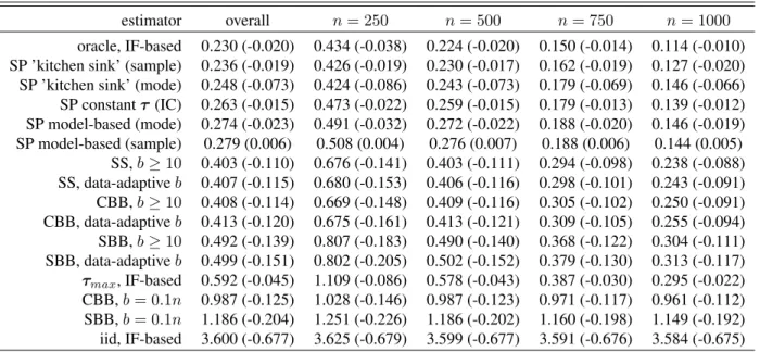
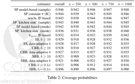
Sieve Plateau Variance Estimators: A New Approach to Confidence Interval Estimation for Dependent Data

They would not only become aware of their own inner strengths and characteristics (Seligman et al., 2009), but they would also feel the use of true partnership of the family

Anti-inflammatory effects of the preparation were studied according to the below methods: S.Salamon– burn induced inflammation of the skin, caused by hot water (80 0 C) in white

Una posible interpretación, obviando las razones inmedia- tas que seguramente tuvo Meyrink para utilizar este escenario en su novela (que son, básicamente, que él habitaba en la

Based on the results, theory surpasses practice in which restructuring TESOL programs is a demand to utilize an optimal integration of a core and complimentary segments of

The instrument contained 13 attitudinal statements related to the newsletter received, measured on a seven-point Likert scale: reactions to the site (newsletter frequency, drop

L1-Japanese L2 learners of English were tested on three prosodic patterns–deaccentuation, a regular high pitch accent (H*), and a contrastive pitch accent (L+H*)–and their link

When the construction sector (which, again, benefits from the increased demand created by greater public expenditure) is excluded, export agriculture (Senegal and Uganda) or

• Develop and communicate a profession wide mantra regarding need for exams and other care. • Manage pricing and communicate value to avoid