Asymptotic properties of Local Polynomial
regression with missing data and correlated
errors
Pérez-González, A.
1∗; Vilar-Fernández, J. M.
2and González-Manteiga, W.
31
Dep. Statistics and Operations Research,(Univ. of Vigo)
Faculty of Business Sciences, Campus South, Ourense, Spain.
e-mail: [email protected]
2
Dep. Mathematics (Univ. of A Coruña)
Faculty of Computer Science, Campus de Elviña, A Coruña, Spain.
e-mail: [email protected]
3
Dep. Statistics and Operations Research
(Univ. of Santiago de Compostela)
Faculty of Mathematics, Campus South, Santiago de Compostela, Spain
e-mail: [email protected]
March 7, 2007
Abstract
The main objective of this work is the nonparametric estimation of the regression function with correlated errors when observations are missing in the response variable. Two nonparametric estimators of the regression function are proposed. The asymptotic properties of these estimators are studied; expresions for the bias and the variance are obtained and the joint asymptotic normality is established. A simulation study is also included.
Keywords: Local Polynomial Regression, Missing Response and Corre-lated Errors
1
Introduction
The local polynomial fitting is a attractive technique used for estimating the regression function. Many authors have studied the asymptotic properties of the local polynomial fitting in a context of dependence (Masry, 1996a; Masry, 1996b; Masry and Fan, 1997; Härdle and Tsybakov, 1997; Hardle et al., 1998; Vilar and Vilar 1998, etc.). A broad study of the local polynomial modelling can be found in Fan and Gijbels (1996).
Most of the statistical methods are designed for complete data sets and problems arise when missing observations are present, which is a common situation in biomedical, environmental or socioeconomic studies, for example. Classic examples are found in thefield of social sciences with the problem of non-response in sample surveys, in Physics, in Genetics (Meng, 2000), etc.
In the regression context, a common method is to impute the incom-plete observations and then proceed to carry out the estimation of the con-ditional or unconcon-ditional mean of the response variable with the completed sample. The methods considered include linear regression (Yates, 1933), ker-nel smoothing (Cheng, 1994; Chu and Cheng, 1995; González-Manteiga and Pérez-González, 2004), nearest neighbor imputation (Chen and Shao, 2000), semiparametric estimation (Wang et al., 2004), nonparametric multiple im-putation (Aerts et al., 2002), empirical likelihood over the imputed values (Wang and Rao, 2002), etc.
For dependent data, the problem of missing observations has been studied using various techniques like the likelihood estimation (Peña and Tiao, 1991; Jones R. H., 1980), least squares (Beveridge, 1992; Chow and Lin 1976; etc.) and kernel estimation (Robinson, 1984), among others.
The objective of this paper is to introduce a nonparametric estimator of the regression function with correlated errors when observations are missing in the response variable. The observations can be missed for various reasons, for example in a time series: the fault of an equipment of measurement, the inability of to observe the series at some instants, for example on holidays or
due to a tempest, etc.
In this paper, we propose two nonparametric estimators when we have missing observations in the response variable based on the local polyno-mial estimator for complete data studied by Francisco-Fernández and Vilar-Fernández (2001) for fixed design and correlated errors.
The first one is the Simplified Local Polynomial Smoother(SLPS), which only uses complete observations. The second one is based on the techniques of simple imputation already used by Chu and Cheng (1995) or González-Manteiga and Pérez-González (2004). This estimator, that we will refer to as Imputed Local Polynomial Smoother (ILPS), consists in using SLPS to estimate the missing observations of the response variableY; then, the local polynomial estimator for complete data is applied to the completed sample. Let us consider thefixed regression model where the functional relation-ship between the design points,xt,n, and the responses,Yt,n, can be expressed
as
Yt,n=m(xt,n) +εt,n, 1≤t≤n,
where m(·)is a regression function defined in[0,1],without any loss of gen-erality, andεt,n, 1≤t ≤n, are unobserved random variables with zero mean
and finite variance, σ2
ε. We assume, for each n, that {ε1,n, ε2,n, ..., εn,n} have
the same joint distribution as { 1, 2, ..., n}, where { t, t∈Z} is a strictly
stationary stochastic process. In this way, it is assumed that the errors of the model can be in general dependent.
The design pointsxt,n, 1≤t ≤n, follow a regular design generated by a
density f. So, for each n, the design points are defined by
Z xt,n
0
f(x)d(x) = t−1
n−1, 1≤t≤n,
where f is a positive function, defined in [0,1] and its first derivative is continuous.
For simplicity, we are going to avoid the subindex n in the sample data and in the errors notation, that is, we are going to use xt,Yt andεt.
The response variable Y can have missing data. To check whether an observation is complete ((xt, Yt)∈R2) or not ((xt,?)), a new variable δ is
introduced into the model as an indicator of the missing observations. Thus, δt= 1 if Yt is observed, and zero if Yt is missing fort = 1, ..., n.
Following the patterns in the literature (see Little and Rubin (1987), etc), we need to establish whether the loss of an item of data is independent or not of the value of the observed data and/or the missing data. In this paper we suppose that the data are missing at random (MAR), i.e.:
P (δt= 1/Yt, xt) =P (δt= 1/xt) =p(xt), (1)
p being a positive function, defined on[0,1]and itsfirst derivative is contin-uous. We suppose that the variablesδt are independent.
In the next section we present the regression model with missing data, as well as the nonparametric estimators used. The Mean Squared Error and the
asymptotic distribution of the estimators are shown in Section 3. In Section 4, a simulation study is presented. The conclusions are shown in Section 5. And, finally Section 6 contains the proofs of the asymptotic results.
2
The regression model and the
nonparamet-ric estimators.
Our goal is to estimate the unknown regression function m(x) and its deriv-atives using weighted local polynomial fitting. We assume that the(p+ 1)th derivative of the regression function at point x exist and are continuous. As indicated previously, two nonparametric estimators are studied, the first (Simplified estimator) arises from using only complete observations and is a generalization of the local polynomial estimator. If we assume that the
(p + 1)th derivatives of the regression function at point x exist and are continuous, the parameter vector β(x) = (β0(x), β1(x),· · · , βp(x))T, where
βj(x) = m(j)(x)/(j!), with j = 0,1, . . . , p, can be estimated by minimizing
the function
where Yn = ⎛ ⎜ ⎜ ⎜ ⎜ ⎝ Y1 .. . Yn ⎞ ⎟ ⎟ ⎟ ⎟ ⎠, Xn= ⎛ ⎜ ⎜ ⎜ ⎜ ⎝ 1 (x1−x) · · · (x1−x)p .. . ... ... ... 1 (xn−x) · · · (xn−x) p ⎞ ⎟ ⎟ ⎟ ⎟ ⎠, Wnδ =diag¡n−1Khn(x1−x)δ1, .., n− 1K hn(xn−x)δn ¢ withKhn(u) =h− 1
n K(h−n1u),Kbeing a kernel function andhnthe bandwidth
or smoothing parameter that controls the size of the local neighborhood and so the degree of smoothing.
Assuming the invertibility of Xt
nWδnXn, the estimator is ˆ βS,n(x) = ¡ XT nWδnXn ¢−1 XT nWδnYn =S−n1Tn, (2)
whereSnis the array(p+1)×(p+1)whose(i, j)th element issi,j,n =si+j−2,n
with sk,n= 1 n n X t=1 (xt−x)kKhn(xt−x)δt, 0≤k ≤2p and Tn = (t0,n, t1,n, ..., tp,n)t, being ti,n = 1 n n X t=1 (xt−x) i Khn(xt−x)Ytδt, 0≤i≤p. (3)
A second estimator (Imputed estimator) is computed in two steps. In the first step, the Simplified estimator with degree q, kernel L and smoothing
parameter gn, is used to estimate the missing observations. In this way, the samplen³xt,Yˆt ´on t=1 is completed, where b Yt=δtYt+ (1−δt)mbS,gn(xt), with mˆS,gn(x) =e t
1βˆS,n(x) andej is the (p+ 1)×1dimensional vector with
1 at the jth coordinate and zero at the rest. Now, the simplified estimation is applied to the data n³xt,Yˆt
´on
t=1 with degree p (p ≥ q), kernel K and smoothing parameter hn. The expression of this estimator is
ˆ βI,n(x) = ¡ XT nWnXn ¢−1 XT nWnYˆn=U−n1Vn, (4) where Yb =³Y1, ..,b Ybn ´T , Wn=diag(n−1Khn(x1−x), .., n− 1K hn(xn−x)).
3
Asymptotic properties.
In this Section asymptotic expressions for the bias and variance/covariance array and the asymptotic normality of the estimate defined in (2) and (4) are obtained. The following assumptions will be needed in our analysis:
A.1. Kernel functionsK and L are symmetric, with bounded support, and Lipschitz continuous.
A.2. The sequence of smoothing parameters, {ln}, with ln satisfies that
ln >0, ln ↓0, nln↑ ∞, where ln=hn or gn.
A.3. DenoteCov( i, i+k) =σε2ν(k), k = 0,1,2...then
P∞
3.1
Asymptotic properties of the Simpli
fi
ed estimator.
The following notations will be used. Let μK,j = R ujK(u)du and ν K,j =
R
ujK2(u)du and let us denote μ
K =
¡
μK,p+1, . . . , μK,2p+1¢T and SK and
˜
SK are the arrays whose (i, j)th elements are sK,i,j = μK,i+j−2 and s˜K,i,j =
νK,i+j−2,respectively.
In the following theorem, expressions for the bias and the variance array of the estimator βˆS,n(x)are obtained.
THEOREM 1. If assumptions A1, A2 and A3 are fulfilled, for every
x∈(hn,1−hn), we have Hn ³ E³βˆS,n(x)/δ ´ −β(x)´= m (p+1)(x) (p+ 1)! h p+1 n S−K1μK+op(hpn+11), (5) with 1 = (1, . . . ,1)T and V ar³HnβˆS,n(x)/δ ´ = 1 nhn cδ(ε) p(x)2f(x)S −1 K ˜SKS−K1(1+op(1)), (6)
where Hn= diag (1, hn, h2n,· · · , hpn), δ = (δ1, .., δn)T and
cδ(ε) =p(x)2c(ε) +p(x)q(x)ν(0)σ2ε, with c(ε) =σ2 ε(ν(0) + 2 P∞ k=1ν(k)) and q(x) = (1−p(x)). Remarks.
estimatormˆ(S,hj)n(x) = (j!)eT j+1βˆS,n(x) is AM SE³mˆ(S,hj)n(x)/δ´ = µ (j!)m(p+1)(x) (p+ 1)! h p+1−j n e T j+1S− 1 K μK ¶2 + (j!) 2 nh2nj+1 cδ(ε) p(x)2f(x)e T j+1S−K1S˜KS−K1ej+1, j = 0, . . . , p.
• The existence of missing observations has no influence on the bias but does on the variances of the estimatorsmˆ(S,hj)n(x) through the term
cδ(ε) p(x)2 = µ c(ε) +q(x) p(x)ν(0)σ 2 ε ¶ ≥c(ε),
which decreases asp(x)increases, and therefore, decreases the variance.
• Expressions (5) and (6) generalize those obtained by Francisco-Fernández and Vilar-Fernández (2001) for the case of complete data (p(x) = 1)
under dependence.
• If the observations are independent, considering thatcδ(ε) =p(x)ν(0)σ2
ε, one obtains AM SE ³ ˆ m(S,hj)n(x)/δ ´ = µ (j!)m(p+1)(x) (p+ 1)! h p+1−j n e T j+1S− 1 K μK ¶2 + (j!) 2 nh2nj+1 ν(0)σ2 ε p(x)f(x)e T j+1S− 1 K S˜KS−K1ej+1.
To establish the asymptotic normality ofβˆS,n(x), the following additional
assumptions are necessary:
A.4. The process of the random errors{εt} has a moving average MA(∞)
-type dependence structure, so
εt=
∞
X
i=0
φiet−i, t= 1,2, . . .
where{et}is a sequence of independent identically distributed random
variables with zero mean and varianceσ2
e,and the sequence{φi}verifies
that P∞i=0|φi|<∞.
A.5. E|et|
2+γ
<∞ for someγ >0
A.6. hn=O(n−1/(2p+3))
A.7. The sequences of smoothing parameters {hn} and {gn} are the same
order, this is, lim
n→∞
hn
gn
=λ.
THEOREM 2. If assumptions A1-A6 are fulfilled, for every x∈(hn,1−
hn), we have the asymptotic normality of βˆS,n(x) conditional on δ :
p nhn µ Hn ³³ ˆ βS,n(x) ´ −β(x)´− m (p+1)(x) (p+ 1)! h p+1 n S−K1μK ¶ L −→N(p+1)(0,ΣS) (7) where ΣS = cδ(ε) p(x)2f(x)S −1 K ˜SKS− 1
K ,and N(p+1)(0,ΣS)denotes a multivariate
The asymptotic normality conditional onδ of the individual components
ˆ
m(S,hj)n(x) = (j!) ˆβS,j(x) is directly derived from Theorem 2. We have, for
j = 0,· · · , p, q nh1+2n j µ³ ˆ m(S,hj)n(x)−m(j)(x)´−hpn+1−jm (p+1)(x) (p+ 1)! (j!)e T j+1S− 1 K μK ¶ L −→N¡0, σ2j¢, where σ2 j = (j!) 2 cδ(ε) p(x)2f(x)e t j+1S− 1 K S˜KS−K1ej+1.
The condition of dependence given in assumption A.4. is very general and a large class of stationary processes have MA(∞) representations (see Section 5.7 of Brockwell and Davis(1991)). This condition is taken on to be able to use a Central Limit Theorem for sequences with m(n)−dependent main part of Nieuwenhuis (1992). A different strategy can be used to obtain the asymptotic normality of the estimator βˆS,n(x). For this, assuming that
the process of the errors {εt} is strong mixing (α−mixing) and imposing
bound conditions on the mixing coefficients, following a similar approach to that employed in Masry and Fan (1997) or Francisco-Fernández and Vilar-Fernández (2001) one can obtain the asymptotic normality of βˆS,n(x) using the well known "small-blocks and large-blocks" method.
3.2
Asymptotic properties of the Imputed estimator.
Considering that
b
where mbS,gn(xi) = ˆm
(0)
S,gn(xi), the following basic decomposition is obtained
ˆ βI,n(x)−β(x) = ¡XTnWnXn ¢−1 XTnWn ⎛ ⎜ ⎜ ⎜ ⎜ ⎝ δ1(Y1−m(x1)) .. . δn(Yn−m(xn)) ⎞ ⎟ ⎟ ⎟ ⎟ ⎠ +¡XT nWnXn ¢−1 XT nWn ⎛ ⎜ ⎜ ⎜ ⎜ ⎝ (1−δ1) ( ˆmS,gn(x1)−m(x1)) .. . (1−δn) ( ˆmS,gn(xn)−m(xn)) ⎞ ⎟ ⎟ ⎟ ⎟ ⎠ +¡XTnWnXn ¢−1 XTnWn ⎛ ⎜ ⎜ ⎜ ⎜ ⎝ m(x1) .. . m(xn) −XTnβ(x) ⎞ ⎟ ⎟ ⎟ ⎟ ⎠ = Γ1 +Γ2+Γ3. (8)
Using it as basis, the conditional asymptotic mean square error ofβˆI,n(x)
is obtained as follows. The following notations will be used. Let L∗gn,q(v) =
eT 1S− 1 L (1, . . . , v q)T Lgn(v) andAj,q(v) = gn R ujK(u)L∗gn,q(hn(v−u))du, and
let us denoteZandZ˜as the arrays whose(i, j)thelements,i, j = 1, . . . , p+1, are zi,j = R Ai−1,q(v)Aj−1,q(v)dv and z˜i,j = R vi−1K(v)A j−1,q(v)dv, respec-tively.
veri-fied. Then, for every x∈(rn,1−rn), with rn= max{hn, gn}, we have Hn ³ E³βˆI,n(x)/δ´−β(x)´ = m (p+1)(x) (p+ 1)! h p+1 n S− 1 K μK (9) +q(x)m (q+1)(x) (q+ 1)! g q+1 n S−K1μ˜Ke1S−L1μL +op ¡ 1(hpn+1+gqn+1)¢
and, if hn andgn verify A7, then
V ar³HnβˆI,n(x)/δ ´ = 1 nhn cδ(ε) f(x)S −1 K (10) µ e SK +λ2 q(x)2 p(x)2Z+ 2λ q(x) p(x) ˜ Z ¶ S−K1(1 +op(1)), whereμ˜K = ¡ μK,0, . . . , μK,p ¢t . Remarks.
• From expressions (9) and (10) it is deduced that the two smoothing parameters used to calculate the estimator βˆI,n(x) have influence in
the expressions of the bias and asymptotic variance. The conditional AM SE of the estimatormˆ(I,hj)n(x) = (j!)eT
AM SE³mˆ(I,hj)n(x)/δ´ = ⎛ ⎜ ⎜ ⎝ (j!)m(p+1)(x) (p+ 1)! h p+1−j n eTj+1S−K1μK+ (j!)m(q+1)(x) (q+ 1)! q(x) gq+1 n hjn eT j+1S− 1 K μ˜Ke1S−L1μL ⎞ ⎟ ⎟ ⎠ 2 + (j!) 2 nh2nj+1 cδ(ε) f(x)e T j+1S− 1 K µ SK+ h2 n g2 n q(x)2 p(x)2Z+ 2 hn gn q(x) p(x) ˜ Z ¶ S−K1ej+1, j = 0, . . . , p.
• The existence of missing observations has influence in the bias and the variances of the estimatormˆ(I,hj)n(x).The expressions (9) and (10)generalize those obtained by Francisco-Fernández and Vilar-Fernández (2001) for the case of complete data (p(x) = 1) under dependence.
• The dependence of the errors influences the variance of the estimator
ˆ
m(I,hj)n(x) through the term cδ(ε). If the observations are independent
one obtains that
AM SE³mˆ(I,hj)n(x)/δ´ = ⎛ ⎜ ⎜ ⎝ (j!)m(p+1)(x) (p+ 1)! h p+1−j n eTj+1S− 1 K μK+ (j!)m(q+1)(x) (q+ 1)! q(x) gq+1 n hjn eT j+1S− 1 K μ˜Ke1S−L1μL ⎞ ⎟ ⎟ ⎠ 2 + (j!) 2 nh2nj+1 c(0)p(x)σ2 ε f(x) e T j+1S− 1 K µ SK+ h2 n g2 n q(x)2 p(x)2Z+ 2 hn gn q(x) p(x) ˜ Z ¶ S−K1ej+1.
This expression generalizes those obtained by González-Manteiga and Pérez-González (2004) who used local linear regression(p=q= 1) for the case of incomplete data under independence.
• In the case gn hn →
0, the expression of the bias is that given in (9) although note that if q = p, the second summand is asymptotically null with respect to the first since gn = o(hn). With respect to the
asymptotic variance, its expression is the following
V ar ³ HnβˆI,n(x)/δ ´ = 1 nhn cδ(ε) p(x)2f(x)S −1 K SeKS− 1 K (1 +op(1)).
This expression coinciding with that obtained for the variance of the Simplified estimator βˆS,n(x) (see 6), hence, if q = p, the estimators, Simplified mˆ(S,hj)n(x) and Imputed mˆ(I,hj)(x), have the same asymptotic mean squared error. But if q < p, the second term of the bias of the Imputed estimator can be dominant, and there, the bias of estimator
ˆ
mI,h(j)n(x) is greater than that of mˆ(S,hj)(x) and also has greaterAM SE.
• In the case of hn gn →
0, again, the expression of the asymptotic bias is that given in (9), but in this case because q ≤p, the second summand on the right side of equation (9) is the dominant term of the bias. To obtain the expression of the variance of the estimator, let us denote R andR˜ as the arrays whose (i, j)th elements,i, j = 1, . . . , p+ 1, are
ri,j = µZ vi+j−2L2(v)dv ¶ µZ vi−1K(v)dv ¶ µZ vj−1K(v)dv ¶ and ˜ ri,j = µZ vi−1K(v)dv ¶ µZ vj−1K(v)dv ¶ ,
respectively. Then, the expression of the variance, in this case, is the following V ar³HnβˆI,n(x)/δ ´ = 1 nhn cδ(ε) f(x)S −1 K µ e SK+ hn gn q(x)2 p(x)2R+ 2 hn gn q(x) p(x) ˜ RL∗q(0) ¶ S−K1(1 +op(1)) ≈ 1 nhn cδ(ε) f(x)S −1 K SeKS−K1(1 +op(1)).
In this case, the Imputed estimator provides better asymptotic variance than the Simplified estimator due to the oversmoothing of the band-width parameter gn. But the bias for the Imputed estimator is bigger
than that for the simplified one.
• From the above, it is deduced that the Imputed estimator gives good results if hn = ξgn is chosen. A selection method of these parameters
consists of to find hn and ξ that minimize the AM SE
³
ˆ
m(I,hj)n(x)/δ´. For example, usingp=qand consideringhn =ϕn−1/(2p+3) as the usual
AM SE³mˆ(I,hj)n(x)/δ´ = AM SE(ϕ, ξ) = ⎛ ⎜ ⎝ (j!)m(p+1)(x) (p+ 1)! ϕ p+1−jnj−2pp+3−1 ¡ eT j+1S− 1 K μK+q(x)ξ q+1 eT j+1S− 1 K μ˜Ke1S− 1 L μL ¢ ⎞ ⎟ ⎠ 2 + (j!)2 c δ(ε) f(x)ϕ 2j+1n2(p2+1p+3−j)eT j+1S− 1 K (11) µ SK+ξ2 q(x)2 p(x)2Z+ 2ξ q(x) p(x) ˜ Z ¶ S−K1ej+1.
• From expression (11), plug-in selections of ϕandξ can be obtained as values that minimize one estimation of the previous function,AM SE\ (ϕ, ξ). This estimation is obtained when substituting in (11) the valuesm(p+1)(x), cδ(ε), p(x) andf(x) for estimations of these.
Taking into account p(x) = P(δ = 1/x) = E(δ/x), this function can be estimated from sample {(xt, δt)nt=1} by a nonparametric regression
method. The estimator of c(ε) = P∞k=−∞E(εt, εt+k) = P∞k=−∞γ(k),
and therefore, the estimation of cδ(ε)can be obtained in several ways.
In any case, we will use the completed sample n³xt,Y˜t
´n t=1
o
, where
˜
Yt = δtYt+ (1−δt) ˆmS,gpilot(xt), and mˆS,gpilot(xt) was computed with
pilot bandwidth gpilot. Using this sample, several procedures can be used to estimate c(ε).
Müller and Statmüller (1988) suggested an estimator forγ(k)based on first order differences of sequenceξt,r= ˜Yt−Y˜t−r, t= 1, . . . , n,with lag
r (r≥1). Supposing that εt is an m-dependent process, Müller and
Statmüller (1988) proved the asymptotic properties of the proposed estimator, γˆMS(k). Now an estimator ˆcM S(ε) for c(ε) is defined as
follows: ˆ cM S(ε) = r(n) X k=r(n) ˆ γM S(k),
wherer(n)is a sequence of positive integers, withr(n)→ ∞asn→ ∞. Under more general conditions of dependence, εt is α−mixing.
Her-mann et al (1992) used second order differences of Y˜t, defined as
ηt,α,β = ˜Yt−
α
α+βY˜t+β− β
α+βY˜t−α,
and they proposed estimatorsˆγHGK(k)for the covariances of the processεt
based on these differences ηt,α,β. Again, an estimatorcˆHGK(ε) for c(ε)
is defined as follows: ˆ cHGK(ε) = r(n) X k=r(n) ˆ γHGK(k).
The consistency of this estimator is proven in Hermann et al (1992). Also, Hall and Van Keilegon (2003) suggested a new difference-based method for estimating error autocovariance with time series errors.
The asymptotic normality of the estimator βˆI,n(x) is established in
THEOREM 4. Assume A1-A7. Then, for every x ∈ (rn,1−rn), we
have the asymptotic normality of βˆI,n(x) conditional on δ :
p nhn ³ Hn ³³ ˆ βI,n(x)´−β(x)´−BI ´ L −→N(p+1)(0,ΣI), where BI = m(p+1)(x) (p+ 1)! h p+1 n S− 1 K μK+q(x) m(q+1)(x) (q+ 1)! g q+1 n S− 1 K μ˜Ke1S−L1μL, and ΣI = cδ(ε) f(x)S −1 K µ e SK+λ2 q(x)2 p(x)2Z+ 2λ q(x) p(x)Z˜ ¶ S−K1.
The asymptotic normality of the individual componentsmˆ(I,hj)n(x) = (j!) ˆβI,j(x)
is directly derived from Theorem 2. Moreover, the considerations made in Theorem 2 with respect to the dependence structure of the errors process are also valid for this estimator.
4
A simulation study
In this section, we compare the performance of the Simplified estimator (2) and the Imputed estimator (4). For this purpose, we use the complete data estimator as reference. The simulation study was carried out using a local linear smoother (p= 1), consideringp=q= 1 for the Imputed estimator.
data and with random errors following an AR(1) process
εt =ρεt−1+et
withN(0, σ= 0.3)distribution. The regression function considered ism(x) = 5(x−0.5)3, and the missing data model (1) is p(x) = 0.8 exp (
−x2). The kernel functions used (K andL) were the Epanechnikov kernel.
To study the influence of the dependence of the observations, different degrees of dependence were considered, specifically, the following correlation coefficient values were considered forρ: ρ=−0.8, −0.5, −0.25, 0, 0.25, 0.5, and 0.8.
In thefirst part of the study the global smoothing parameters needed for the three estimators were estimated. For this, the Mean Integrated Square Error, MISE, was considered as error criterion. Three hundred samples, of size 100, of the previous model were generated, and the MISE value was approached by Montecarlo for each smoothing parameter value taken over a grid of size 100 of interval(0,1). For the Imputed estimator the minimization process was carried out using a double grid for the smoothing parameters used (hn and gn). Table 1 shows the values obtained for the optimal global
smoothing parameters for each correlation coefficient (ρ) value.
INSERT Table 1 ABOUT HERE.
Simplified estimator, it is apparent how the missing data imply an increase in the smoothing parameter. For another hand, for the three estimators, we can observe that when the dependence of the observations increases, that is, the value of ρ increases, then, the variability of the data increases, and therefore, the optimal smoothing parameter also increases.
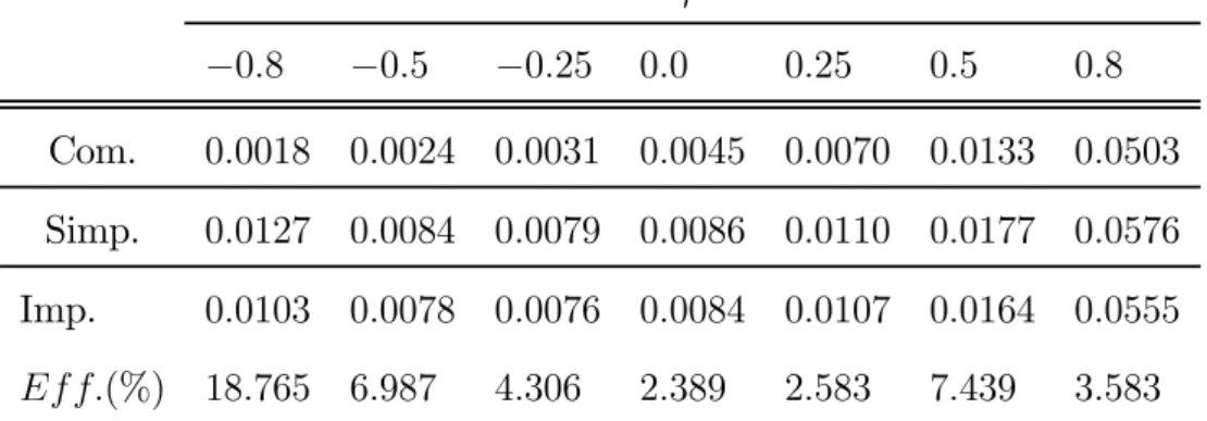
Once the optimal bandwidths are obtained, the estimation of the regres-sion function was carried out on another 500 different samples. For these samples, the Mean Squared Error and the MISE were estimated. To com-pare the Simplified and the Imputed estimators we computed the efficiency of the latter in the following way:
Ef f.(%) = M ISESIM P −M ISEIM P U T
M ISESIM P ×
100, obtaining the values observed in the last row of Table 2.
INSERT Table 2 ABOUT HERE.
The results show better behavior for the Imputed estimator than for the Simplified, with a benefit above 2.5%. Just as in the case of complete data, we see that as the correlation coefficient increases, the value of the MISE increases drastically.
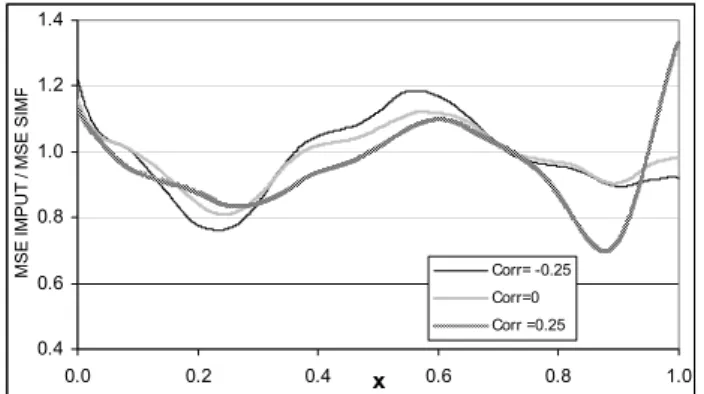
Figure 1 shows the quotient between the Mean Squared Errors, MSE, for Imputed and for Simplified estimators for three correlation coefficient values (ρ=−0.25,0and 0.25). It is apparent that at certain points the Simplified
estimator is better than the Imputed. This finding, along with the fact that when using global measures such as the MISE, the Imputed estimator is better, justifies that selection of a local bandwidth (for each point) would substantially improve the results.
INSERT Figure 1 ABOUT HERE.
Figure 2 shows the boxplots of the MSE for the three estimators with ρ=−0.25,0 and0.25.
INSERT Figure 2 ABOUT HERE.
It is observed that as the correlation coefficient increases, the MSE also increase. Moreover, the good behavior of the Imputed estimator is apparent compared with the Simplified in the three cases.
4.1
The e
ff
ect of strong dependence
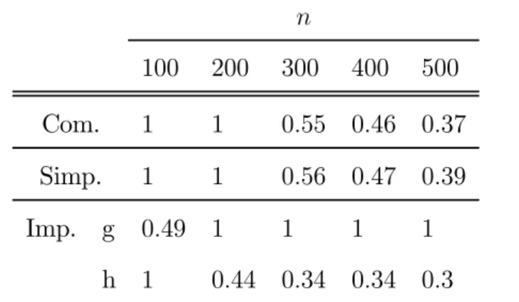
We were interested in studying the behavior of the estimators under strong dependence for different sample sizes. For this reason, we performed more simulations using larger sample size for this value (ρ = 0.8). The following tables show the optimal bandwidth and the MISE obtained for several sample sizes.
INSERT Table 3 ABOUT HERE. INSERT Table 4 ABOUT HERE.
We can see that as the sample size increases, the MISE decreases and the behavior of the Imputed estimator is better. The bandwidth for the imputa-tion of the Imputed estimator (gn) is very big because when the correlation
is big, the variance is big also. In the asymptotic results we can see that if we choose hn
gn →
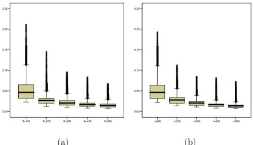
0the variance for the Imputed estimator is lower than that for the Simplified estimator. The oversmoothing tends to decrease the variance. The followingfigures show the boxplots of the Mean Squared Error (MSE) for the estimators for incomplete data, and for five sample sizes.
INSERT Figure 3 ABOUT HERE.
The two estimators have similar behavior with respect to sample size, as long as ngrows the MSE decreases.
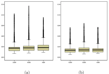
If we compare the three estimators (complete data case, Simplified and Imputed estimators) for various sample sizes, we see the following graphs.
INSERT Figure 4 ABOUT HERE.
The complete data case has the best behavior, and the Imputed estimator performs better than the Simplified estimator.
5
Conclusions
In this paper we have proposed two nonparametric estimators of the regres-sion functions with correlated errors and missing observations in the response variable. The Mean Squared Error and the asymptotic normality of the esti-mators have been studied. We observed that the performance of the estima-tors depends on the bandwidth parameters. The Imputed estimator needs two bandwidth parameters, and when a suitable choice of these parameters is made, the behavior of this one is better than that of the Simplified one. In the case of the imputation and the estimation bandwidth verify gn
hn →
0, the Simplified estimator is better than the Imputed estimator. In the case of hn
gn →
0, the Imputed estimator has a smaller variance but the bias can be bigger. Nevertheless, if the bandwidth parameters are of similar order (hn = ξgn with ξ > 0) , the Imputed estimator can be better than the
Simplified estimator.
6
Proofs.
In this section, we sketch proofs of the results presented in Section 3. First, the convergence for arraysSn andTn are established.
(hn,1−hn), we have
lim
n→∞H −1
n SnH−n1 =p(x)f(x)SK(1+op(1)). (12)
PROPOSITION 2. Under assumptions A1, A2 and A3, for everyx∈
(hn,1−hn), we have lim n→∞nhnV ar ¡ H−n1Tn/δ ¢ =p(x)f(x)S˜K(1+op(1)).
Using Taylor’s expansion and following a similar approach to that em-ployed in Francisco-Fernández and Vilar-Fernández (2001) we can deduce Propositions 1 and 2.
Proof of Theorem 1.
Let Mn = (m(x1), ..., m(xn)) t
. Performing a (p+ 1)th−order Taylor expansion of function m in a neighborhood ofx, we obtain
E³βˆS,n(x)/δ´−β(x) = ¡XT nW δ nXn ¢−1 XT nW δ n ¡ Mn−Xtnβ ¢ = m (p+1)(x) (p+ 1)! ¡ XT nW δ nXn ¢−1 ⎛ ⎜ ⎜ ⎜ ⎜ ⎝ ⎛ ⎜ ⎜ ⎜ ⎜ ⎝ sp+1,n . . . s2p+1,n ⎞ ⎟ ⎟ ⎟ ⎟ ⎠+op ¡ hpn+11¢ ⎞ ⎟ ⎟ ⎟ ⎟ ⎠.
Using Proposition 1 we obtain the bias of βˆS,n(x)given in (5).
Again, using (12) we have
V ar³βˆS,n(x)/δ´= 1
p(x)2f(x)1H
−1
n SKH−n1V ar(Tn/δ)Hn−1SKH−n1(1+op(1)).
(13) From (13) and Proposition 2, we deduce the expression of the conditional variance of βˆS,n(x) (6).
Proof of Theorem 2.
First, we study the asymptotic distribution conditional onδ of the vector √
nhn(H−n1(T∗n)), where (Tn∗) = (Tn)−E (Tn/δ). For it, let QS,n be an
arbitrary linear combination of
H−n1(T∗n), QS,n=˜aT ¡ H−n1(T∗n)¢= p X i=0 αih−ni((ti,n)−E(ti,n/δ)) with ˜a= (a0, a1, . . . , ap)∈Rp+1. So p nhnQS,n = n X t=1 ξt,n, where ξt,n = r hn n Ψhn(xt−x)δtεt, with Ψ(u) =K(u) p X i=0 αiuj and Ψhn(u) = 1 hn Ψ µ u hn ¶ .
Using Proposition 2, the variance ofQS,n is obtained σ2QS = lim n→∞V ar(QS,n/δ) = limn→∞nhn˜a TV ar¡H−1 n (T∗n/δ) ¢ ˜ a=p(x)f(x)S˜K <∞. (14) It remains to prove the asymptotic normal distribution conditional onδ
of QS,n =
Pn
t=1ξt,n. For it, we will use the following Central Limit Theorem
for sequences with m(n)−dependent main part of Nieuwenhuis (1992).
Theorem A.5.Suppose that the array {Xi,n, 1≤i≤q(n)}has anm(n)−dependent
main part
n
˜
Xi,n
o
and a residual part ©X¯i,n
ª . Set b2n = V ar ³Pq(n) i=1 Xi,n ´ .
Assume that the arrays (Xi,n/bn) and
¡¯
Xi,n/bn
¢
satisfy the variance condi-tions C1 and C∗1,respectively, and that both arrays satisfy the (2+δ)-moment
condition C2 for some δ >0 with m(n)2+2/δ/q(n)→0. Then
1 bn q(n) X t=1 (Xt,n−E(Xt,n))−→L N(0,1) as n→ ∞.
The above conditions are:
Condition C1. max i<j≤q(n) 1 j−iV ar( j P t=i+1 Xt,n bn ) =O( 1 q(n)) as n→ ∞. Condition C∗1. max i<j≤q(n) 1 j−iV ar( j P k=i+1 ¯ Xt,n bn ) =o( 1 q(n)) as n→ ∞. Condition C2. max 1<t≤q(n)E(|Zt,n| 2+γ ) =O(q(n)−1−(γ/2)) as n→ ∞,
with Zt,n= Xt,n bn or ¯ Xt,n bn .
Here an array Zt,n is called m(n)−dependent if for all n ∈ N and k ∈
{2, . . . , q(n)−m(n)} the random vectors (Zt,n: 1≤t≤k−1) and
(Zi,n:k+m(n)≤i≤q(n)) are independent. The sequence m(n) verifies
m(n)/n→0 asn→ ∞.
In our case, using assumption A.4. we have
εt= ∞ X i=0 φiet−i = mX(n) i=0 φiet−i+ ∞ X i=m(n) φiet−i = ˜εt+ ¯εt.
Then, taking into account that the kernelK has bounded support, chang-ing the indices and without loss of generality, it can be written as
p nhnQS,n = |Xhnn| t=−|hnn| ξt,n = |Xhnn| t=−|hnn| (ˆξt,n+ ¯ξt,n),
where q(n) = 2|hnn| (|•| denotes the integer part), ξt,n is a triangular array
with m(n)−dependent main part ˆξt,n and residual part ¯ξt,n, obtained when substituting inξt,n, εt for˜εt and¯εt,respectively.
In the following, we shall prove that our array verifies the conditions of Theorem A.5.
Condition C1. Under A.1, A.3 and using (14) we obtain 1 j−iV ar( j P t=i+1 ξt,n bn )≤ 1 j−i 1 b2 n j P t=i+1 j P k=i+1 E¡ξt,nξk,n ¢ ≤ jC −i 1 nhn j−P(i+1) s=−(j−i−1) (j −i−|s|)|ν(s)|=O( 1 nhn ) =O( 1 q(n)),
where C is a positive constant (notation that will be used from here on). Therefore, ©ξt,n/bn
ª
verifies C1.
Condition C∗
1. Reasoning in a similar way, it is easy to show that
1 j−iV ar( j P t=i+1 ¯ ξt,n bn )≤ 1 j−i 1 b2 n j P t=i+1 j P k=i+1 E¡¯ξt,n¯ξk,n ¢ ≤ nhC n j−P(i+1) s=−(j−i−1) E(¯εt,n¯εt+s,n) = C nhn j−P(i+1) s=−(j−i−1) P j>m(n) φj P k>m(n) φkE(et−jek−j) ≤ nhC n P s ( P j>m(n) φjφj+s)σ 2 e ≤ C nhn à P j>m(n) φj !2 =o( 1 nhn ) =o( 1 q(n)).
Condition C2.We want to prove(2+γ)−moment condition for the arrays ξt,n/bnand¯ξt,n/bn.This is done for thefirst one, but for the second, an similar
approach is used. Taking into account the form of the function Ψhn(u),
E ¯ ¯ ¯ ¯ ξt,n bn ¯ ¯ ¯ ¯ 2+γ =C E ¯ ¯ ¯ ¯ 1 √ nhn εt ¯ ¯ ¯ ¯ 2+γ =O µ 1 √ nhn ¶2+γ =O(q(n)−1−(γ/2)).
Therefore, we have proven the asymptotic normality conditional onδ of
QS,n=
p
nhn˜aT
¡
H−n1(T∗n)¢−→L N(0, σ2QS).
Now, using the Cramer-Wold Theorem we obtain the asymptotic normal-ity conditional on δ of
p
nhn
¡
H−n1(T∗n)¢−→L N(p+1)(0,ΣS). (16)
Finally, taking into account
p nhnHn ³³ ˆ βS,n(x)´−β(x)´ =pnhn ¡ H−n1SnH−n1 ¢−1 H−n1(T∗n) +pnhnHn ³ E³βˆS,n(x)/δ ´ −β(x)´
from (5) and (16) and using Proposition 1, the asymptotic normality of the estimatorβˆS,n(x) conditional onδ (given in (7)) is established.
Proof of Theorem 3.
To obtain the bias ofβˆI,n(x), from (8) it follows that
HnE
³
ˆ
because Γ3 is no random term.
From (5) and using Proposition 1 it is easy to obtain that
HnE(Γ2/δ) =q(x) m(q+1)(x) (q+ 1)! g q+1 n S− 1 Kμ˜Ke1S− 1 L μL+1g q+1 n . (18)
Again, using Proposition 1 we have
HnE(Γ3/δ) = m(p+1)(x) (p+ 1)! h p+1 n S− 1 K μK +1h p+1 n (19)
From (17), (18) and (19) it follows (9).
With respect to the variance ofβˆI,n(x), we have
V ar³βˆI,n(x)/δ´=V ar(Γ1/δ) +V ar(Γ2/δ) + 2Cov(Γ1Γ2/δ). Using the same kind of arguments as those used in the proof of (6) we obtain V ar(Γ1/δ) = 1 nhn cδ(ε) f(x)H −1 n S− 1 K eSKS−K1H− 1 n (1 +op(1)). (20)
With respect to the variance ofΓ2,we have
V ar(Γ2/δ) =¡XT nWnXn ¢−1 V ar(Tˆn/δ) ¡ XT nWnXn ¢−1 , where Tˆn= ¡ˆ t0,n,ˆt1,n, ...,ˆtp,n ¢T , being
ˆ tj,n = 1 n n X i=1 (xi−x)j(1−δi)Khn(xi−x) ( ˆmS,gn(xi)−m(xi)), 0≤j ≤p. (21) Using the approximation of the local polynomial estimator by equivalent kernels (see Section 3.2.2 of Fan and Gijbels (1996))mˆS,gn(xi)can be written
as ˆ mS,gn(xi) = n X s=1 Ψδ(xs−xi gn )Ys = 1 nf(xi)p(xi) n X s=1 L∗gn,q(xs−xi)δsYs(1 +op(1)). (22) From (21) and (22) it follows that
Cov¡h−njtˆj,n, h−nktˆk,n/δ ¢ = 1 n4hj+k n X i Khn(xi−x) (1−δi) (xi−x) j ·X t Khn(xt−x) (1−δt) (xt−x) k 1 f(xi)p(xi) 1 f(xt)p(xt) ·X s L∗gn,q(xs−xi)δs X r L∗gn,q(xr−xt)δrc(|s−r|) = ∆1+∆2+∆3+∆4, (23)
where we have split Cov¡h−njtˆj,n, h−nkˆtk,n
¢
into four terms: in ∆1 we have considered the case s = r and i = t; in ∆2, s = ri 6= t; in ∆3, s 6= r i = t;
Developing each of these four terms, we obtain that ∆1 = O µ 1 n2g2 n ¶ , ∆2 = σ2εc(0) f(x)q(x)2 np(x) hn g2 n Z Aj,q(v)Ak,q(v)dv(1 +op(1)), ∆3 = O µ 1 n2g2 n ¶ , ∆4 = 1 n ¡ c(ε)−σ2εc(0) ¢ q(x)2 hn g2 n f(x) Z Aj,q(v)Ak,q(v)dv(1 +op(1)). Therefore, V ar(Tˆn/δ) = hn ng2 n f(x)q(x) 2 p(x)2c δ(ε)Z(1 +o p(1)). (24)
From (24) and Proposition 1, we deduce that
V ar(Γ2/δ) = hn ng2 n 1 f(x) q(x)2 p(x)2c δ(ε)H−1 n S− 1 K ZS− 1 K H −1 n (1 +op(1)). (25)
Finally, we study the termCov(Γ1Γ2/δ),
Cov(Γ1Γ2/δ) = ¡ XtnWnXn ¢−1 Cov(TnT˜tn/δ) ¡ XtnWnXn ¢−1 , (26)
where Tn is given in (3) and T˜n= ¡˜ t0,n,˜t1,n, ...,˜tp,n ¢t , being ˜ ti,n= 1 n n X t=1 (xt−x)iKhn(xt−x) ( ˆmS,gn(xt)−m(xt)) (1−δt), 0≤i≤p.
Using (22) we can expand the terms of matrix Cov(TnT˜tn/δ), and we
have Cov¡h−njtˆj,n, h−nktˆk,n/δ ¢ = 1 n2h−j−k n X i Khn(xi−x) (xi−x) j δi X t Khn(xt−x) ·(xt−x)k(1−δt) X s Ψδ(xs−xt gn )Cov[εi, εs] = Λ1 +Λ2,
where in ∆1 we assume that i=s, and in ∆1 we consider i6=s. Simple algebraic expansions allow us to obtain that
Λ1 = σ2 εc(0)q(x) ngn f(x) Z K(v)vjAk,q(v)dv(1 +op(1)).
Using Taylor expansions we have
Λ2 = (c(ε)−σ2εc(0)) n p(x)q(x)f(x) 1 gn µZ K(v) (v)jAk,q(v)dv ¶ (1 +op(1)).
Hence, Cov¡h−njtˆj,n, h−nktˆk,n/δ ¢ = 1 ngn f(x)q(x) p(x)c δ(ε) Z K(v)vjAk,q(v)dv(1 +op(1)), and Cov(H−n1TnH−n1T˜ t n/δ) = 1 ngn f(x)q(x) p(x)c δ (ε)Z˜(1 +op(1)). (27)
From (26), (27) and using again Proposition 1, we conclude that
Cov(Γ1Γ2/δ) = 1 ngn f(x)q(x) p(x)c δ (ε)H−n1S−K1ZS˜ −K1H−n1(1 +op(1)).
By substituting (20), (25) and (27) in it follows (10).
Proof of Theorem 4.
The same method as that used in the demonstration of Theorem 2 is followed, p nhnHn ³³ ˆ βI,n(x)´−β(x)´=pnhn ¡ H−n1UnH−n1 ¢−1 H−n1χ˜n,
where χ˜ = (χ0,n,χ1,n, . . . ,χp,n), with χj,n = 1 n n X t=1 (xt−x)jKhn(xt−x) ⎛ ⎜ ⎝δtεt + (1−δt) (mbS,gn(xt)−E(mbS,gn(xt)/δ)) ⎞ ⎟ ⎠ 0≤j ≤p.
Using Proposition 1 it is sufficient to prove the asymptotic normality conditional on δ of term √nhnHn−1χ˜. For it, let QI,n be an arbitrary linear
combination of H−1 n χ˜n, QI,n=˜aTH−n1χ˜n= p X i=0
aih−niχi,n, with a˜= (a0, a1, . . . , ap)∈Rp+1.
Using the approximation given in (22) we have
p nhnQI,n= p nhn p X i=0 ai(ui,n+vi,n) = p nhn˜aT(˜un+v˜n),
where u˜n = (u0,n, . . . , up,n)T and ˜vn= (v0,n, . . . , vp,n)T with
ui,n= 1 n n X t=1 µ xt−x hn ¶i Khn(xt−x)εt, 0≤i≤p,
vi,n= 1 n n X t=1 µ xt−x hn ¶i Khn(xt−x) · Ã 1−δt nf(xt)p(xt) n X s=1 L∗gn,q(xs−xt)δsεs ! , 0≤i≤p.
First, we compute the variance ofQI,n.By (20), (25) and (26) and using
the assumption A.7. we obtain
σ2IS = lim n→∞V ar(QI,n/δ) = limn→∞nhn˜a tV ar¡(u˜+˜v)(u˜+v˜)t/δ¢˜a = c δ(ε) f(x)˜a t (SeK +λ2 q(x)2 p(x)2Z+ 2λ q(x) p(x) ˜ Z)˜a. (28)
Expanding the termQI,n we obtain
p nhnQI,n = n X t=1 ηt,n = r hn n Ψhn(xt−x) Ã δtεt+ 1−δt nf(xt)p(xt) n X s=1 L∗gn,q(xs−xt)δsεs ! .
Again, taking into account the form of functions Ψhn(u) and L∗gn,q(u),
that the kernels K and L have bounded support, reordering the sums and if λ = 1, we have p nhnQI,n = |Xhnn| t=−|hnn| ζt,n = |Xhnn| t=−|hnn| (ˆζt,n+ ¯ζt,n),
with ζt,n= r hn n Ψhn(xt−x)δt ⎛ ⎝1 + 1−δt nf(xt)p(xt) |hXnn|−t j=−|hnn|+t L∗gn,q(xt−xj) ⎞ ⎠εt,
where q(n) = 2|hnn| , ζt,n is a triangular array with m(n)−dependent main
part ζˆt,n and residual part ¯ζt,n obtained when substituting in ζt,n, εt by ˜εt
and ¯εt, respectively.
Under assumption A.1. and A.7. we have
ζt,n =
r
hn
n Ψhn(xt−x)δt(1 +C)εt =ξt,n(1 +C). (29)
Using (28) and (29) and reasoning in a similar way as that in the proof of Theorem 2, it is easy to prove that the arrays ζt,n and ¯ζt,n satisfy the
conditions of Theorem A.5. Now the proof of Theorem 4 is complete.
Acknowledgement
Research of the authors was supported by the DGICYT Spanish Grant MTM2005-00429 and MTM2005-00820 (European FEDER support included) and XUGA Grants PGIDT03PXIC10505PN and PGIDT03PXIC20702PN. The authors also wish to thank the referee. His detailed report led to a considerable improvement of the paper.
References
Aerts, M.; Claeskens, G.; Hens, N. and Molenberghs, G. (2002) Local Multile Imputation. Biometrika, 89, 2, 375-388.
Beveridge, S. (1992) Least squares estimation of missing values in time series. Communications in Statistics. Theory and Methods, 21, 12, 3479— 3496.
Brockwell P.J. and Davis R. A. (1991) Time series. Theory and methods (second edition) Springer.
Chen, J. H. and Shao, J. (2000) Nearest neighbor imputation for survey data. Journal of Official Statistics, 16, 113-131.
Cheng, P. E. (1994) Nonparametric estimation of mean functionals with data missing at random. Journal of the American Statistical Association, 89, 425, 81-87.
Chow, G. C. and Lin, A. L. (1976) Best linear unbiased estimation of missing observations in an economic time series. Journal of the American Statistical Association, 71, 355, 719—721.
Chu, C. K. and Cheng, P. E. (1995) Nonparametric regression estimation with missing data. Journal of Statistical Planning and Inference, 48, 85-99.
Fan, J.; Gijbels, I.(1996) Local polynomial modelling and its applications Chapman and Hall, London.
Francisco-Fernández, M. and Vilar-Fernández, J. M. (2001) Local poly-nomial regression estimation with correlated errors. Communications in Sta-tistics. Theory and Methods, 30 , no. 7, 1271—1293.
Glasser, M. (1964) Linear regression analysis with missing observations among the independent variables. Journal of the American Statistical Asso-ciation, 59, 834-844.
González-Manteiga, W. and Pérez-González, A.(2004) Nonparametric mean estimation with missing data. Communications in Statistics. Theory and Methods, 33, 2, 277-303.
Hall, P., and Van Keilegom,I. (2003), Using differences based methods for inference in nonparametric regression with time-series errors. Journal of the Royal Statistical Society: Series B, 65, 443-456.
Härdle, W.and Tsybakov, A. (1997) Local polynomial estimators of the volatility function in nonparametric autoregression. Journal of Econometrics, 81, 1, 223-242.
Härdle, W.; Tsybakov, A. and Yang, L.(1998) Nonparametric vector au-toregression. Journal of Statistical Planning and Inference 68, 2, 221—245.
Herrmann, E., Gasser, T. and Kneip, A. (1992), Choice of bandwidth for kernel regression when residuals are correlated. Biometrika, 79, 4, 783-795.
Ibrahim, J. G. (1990) Incomplete data in generalized linear models. Jour-nal of the American Statistical Association, 85, 411, 765-769.
Jones, R. H. (1980) Maximum likelihoodfitting of ARMA models to time series with missing observations. Technometrics 22, 3, 389—395.
Little R. J. A. (1992) Regression with missing X´s: a review. Journal of the American Statistical Association, 87, 1227-1237.
Little, R. J. A.; Rubin, D. B. Statistical analysis with missing data, J. Wiley & Sons, New York, 1987.
Masry, E. (1996a) Multivariate local polynomial regression for time series: uniform strong consistency and rates. Journal of Time Series Analysis, 17,
6, 571—599.
Masry, E. (1996b) Multivariate regression estimation–local polynomial fitting for time series. Stochastic Process. Appl. 65, 1, 81—101.
Masry, E. and Fan, J. (1997) Local polynomial estimation of regression function for mixing processes. Scandinavian Journal of Statistics. Theory and Applications, 24, 165—179.
Meng, X.-L. (2000). Missing data: Dial M for ???. Journal of the Amer-ican Statistical Association, 95, 452, 1325-1330.
Müller, H. and Stadtmüller, U. (1988), Detecting dependencies in smooth regression models. Biometrika, 75, no. 4, 639-650.
Nieuwenhuis, G. (1992), Central limits theorems for sequences with m(n)-dependent main part. Journal of Statistical Planning and Inference, 32, 229-241.
Peña, D. and Tiao, G. C. (1991) A note on likelihood estimation of missing values in time series. The American Statistician 45, 3, 212—213.
Robinson, P. M. (1984) Kernel estimation and interpolation for time se-ries containing missing observations. Annals of the Institute of Statistical Mathematics, 36, 1, 403—417.
Rubin, D. B. (1987) Multiple imputation for nonresponse in surveys. Wi-ley Series in Probability and Mathematical Statistics: Applied Probability and Statistics. New York: John Wiley & Sons.
Vilar, J. and Vilar, J. (1998) Recursive estimation of regression function by local polynomial fitting. Annals of the Institute of Statistical
Mathemat-ics, 50, 4, 729-754.
Wang, Q.; Linton, O. and Härdle, W. (2004) Semiparametric regression analysis with missing response at random. Journal of the American Statisti-cal Association, 99, 466, 334—345.
Wang, W. and Rao, J. N. K. (2002). Empirical likelihood-based inference under imputation for missing response data. Annals of Statistics, 30,3, 896-924.
Yates, F. (1933) The analysis of replicated experiments when the field results are incomplete. Empire Journal of Experimental Agriculture, 1, 129-142.
TABLES ρ −0.8 −0.5 −0.25 0.0 0.25 0.5 0.8 Com. 0.17 0.19 0.20 0.23 0.26 0.35 1.00 Simp. 0.38 0.32 0.31 0.32 0.36 0.47 1.00 Imp. g 1.00 0.51 0.49 0.51 1.00 1.00 0.49 h 0.21 0.17 0.17 0.19 0.22 0.28 1.00
Table 1: Optimal global bandwidth.
ρ −0.8 −0.5 −0.25 0.0 0.25 0.5 0.8 Com. 0.0018 0.0024 0.0031 0.0045 0.0070 0.0133 0.0503 Simp. 0.0127 0.0084 0.0079 0.0086 0.0110 0.0177 0.0576 Imp. 0.0103 0.0078 0.0076 0.0084 0.0107 0.0164 0.0555 Ef f.(%) 18.765 6.987 4.306 2.389 2.583 7.439 3.583
n 100 200 300 400 500 Com. 1 1 0.55 0.46 0.37 Simp. 1 1 0.56 0.47 0.39 Imp. g 0.49 1 1 1 1 h 1 0.44 0.34 0.34 0.3
Table 3: Optimal bandwidth with correlationρ= 0.8
n
100 200 300 400 500
Com. 0.0503 0.0303 0.0235 0.0188 0.0161
Simp. 0.0576 0.0334 0.0258 0.0205 0.0174
Imp. 0.0555 0.0325 0.0244 0.0193 0.0163
FIGURES
Figure 1: Quotient between Mean Squared Errors for Imputed and Sim-plified estimators withρ=−0.25, 0and0.25.
Figure 2: Boxplots of MSE for the Complete (red), Simplified (green) and Imputed (blue) estimators with ρ=−0.25,0 and0.25.
Figure 3: Boxplots of MSE for Simplified (a) and Imputed (b) estimators with ρ= 0.8andn= 100, 200,300,400 and500.
Figure 4: Boxplots of MSE for the Complete (boxplot on the left), Sim-plified (middle) and Imputed (right) estimators with ρ = 0.8, n = 200(a) and n= 300 (b). 0.4 0.6 0.8 1.0 1.2 1.4 0.0 0.2 0.4 x 0.6 0.8 1.0 M S E IM P U T / M SE SI M P Corr= -0.25 Corr=0 Corr =0.25
Figure 1: Quotient between Mean Squared Error for Imputed and Simplified estimators withρ=−0.25, 0and0.25..
Correlation
.25 .00
-.25
Mean Squared Error
.03 .02 .01 0.00 COMP SIMP IMPUT
Figure 2: Boxplots of MSE for the Complete (red), Simplified (green) and Imputed (blue) estimators with ρ=−0.25, 0 and0.25.
Sn100 Sn200 Sn300 Sn400 Sn500 0,00 0,05 0,10 0,15 0,20 0,25 (a)
In100 In200 In300 In400 In500 0,00 0,05 0,10 0,15 0,20 0,25 (b)
Figure 3: Boxplots of MSE for Simplified (a) and Imputed (b) estimators with ρ= 0.8 andn= 100, 200,300,400 and 500.
Cn200 Sn200 In200 0,00 0,03 0,06 0,09 0,12 0,15 (a) Cn300 Sn300 In300 0,00 0,03 0,06 0,09 0,12 0,15 (b)
Figure 4: Boxplots of MSE for the Complete (boxplot on the left), Simplified (middle) and Imputed (right) estimators withρ= 0.8,