into finite difference methods for option pricing under
L´
evy processes
Oleg Kudryavtsev
To cite this version:
Oleg Kudryavtsev. An implementation of the Wiener-Hopf factorization into finite difference methods for option pricing under L´evy processes. [Research Report] RR-7873, INRIA. 2012, pp.37. <hal-00665482>
HAL Id: hal-00665482
https://hal.inria.fr/hal-00665482
Submitted on 2 Feb 2012HAL is a multi-disciplinary open access archive for the deposit and dissemination of sci-entific research documents, whether they are pub-lished or not. The documents may come from teaching and research institutions in France or abroad, or from public or private research centers.
L’archive ouverte pluridisciplinaire HAL, est destin´ee au d´epˆot et `a la diffusion de documents scientifiques de niveau recherche, publi´es ou non, ´emanant des ´etablissements d’enseignement et de recherche fran¸cais ou ´etrangers, des laboratoires publics ou priv´es.
2 4 9 -6 3 9 9 IS R N IN R IA /R R --7 8 7 3 --F R + E N G
RESEARCH
REPORT
N° 7873
February 2012Wiener-Hopf
factorization into finite
difference methods for
option pricing under
Lévy processes
CENTRE DE RECHERCHE
factorization into finite difference methods for
option pricing under Lévy processes
Oleg Kudryavtsev
∗Project-Team Mathfi
Research Report n° 7873 — February 2012 — 37 pages ∗
Department of Informatics, Russian Customs Academy Rostov Branch, Budennovskiy 20, Rostov-on-Don, 344002, Russia. MATHRISK, INRIA Rocquencourt, France E-mail: [email protected]
based on a finite difference approximation for the generalized Black-Scholes equa-tion. The goal of the paper is to incorporate the Wiener-Hopf factorization into finite difference methods for pricing options in Lévy models with jumps. The method is applicable for pricing barrier and American options. The pricing problem is reduced to the sequence of linear algebraic systems with a dense Toeplitz matrix; then the Wiener-Hopf factorization method is applied. We give an important probabilistic interpretation based on the infinitely divisible distributions theory to the Laurent operators in the correspondent factorization identity. Notice that our algorithm has the same complexity as the ones which use the explicit-implicit scheme, with a tridiagonal matrix. However, our method is more accurate. We support the advan-tage of the new method in terms of accuracy and convergence by using numerical experiments.
Key-words: Lévy processes, barrier options, American options, Wiener-Hopf factorization, finite difference schemes, numerical methods
factorisation de Wiener-Hopf pour l’évaluation
d’options dans des modèles de Lévy
Résumé : On considère le problème d’évaluation d’options pour une large classe de processus de Lévy. On propose une approche numérique basée sur une approximation par différences finies pour l’équation de Black-Scholes généralisée. Le but est d’introduire la factorisation de Wiener-Hopf dans la méthode de différences finies pour l’évaluation d’options dans des modèles de Lévy avec sauts. La méthode s’applique au cas des options barrières et les options américaines. Le problème d’évaluation se réduit à une suite de systèmes linéaires algébriques avec matrice dense de Toeplitz, pour laquelle la méthode de factorisation de Wiener-Hopf est appliquée. Nous donnons une interprétation probabiliste basée sur la théorie des distributions infini-ment divisibles des opérateurs de Laurent de l’identité de factorisation cor-respondante. Notre algorithme a la même complexité que le shéma explicite avec matrice tridiagonale, mais est plus précis. Nous illustrons l’avantage de cette méthode en termes de précision et convergence, sur des expériences numériques.
Mots-clés : Processus de Lévy, options barrières, options américaines, fac-torisation de Wiener-Hopf, méthodes de différences finies, méthodes numériques
1
Introduction
In recent years more and more attention has been given to stochastic models of financial markets which depart from the traditional Black-Scholes model. We concentrate on one-factor non-gaussian exponential Lévy models. These models provide a better fit to empirical asset price distributions that typi-cally have fatter tails than Gaussian ones, and can reproduce volatility smile phenomena in option prices. For an introduction to applications of these models applied to finance, we refer to [7, 14].
Option valuation under Lévy processes has been dealt with by a host of researchers, therefore, an exhaustive list is virtually impossible. However, the pricing of barrier options in exponential Lévy models still remains a mathematical and computational challenge (see, e.g., [33, 22, 23, 4] for recent surveys of the state of the art of exotic option pricing in Lévy models).
The most general method to price barrier or American options under ex-ponential Lévy processes deals with solving the corresponding partial integro-differential equation (the generalized Black-Scholes equation) with appropri-ate boundary conditions. Note that in the case of American options free boundary problem arises. There are four main numerical methods for solv-ing PIDE: multinomial trees, finite difference schemes, Galerkin methods and numerical Wiener-Hopf factorization methods.
In [1], it is constructed a family of Markov chain approximations of jump-diffusion models. Multinomial trees can be considered as special cases of explicit finite difference schemes. The main advantage of the method is simplicity of implementation; the drawbacks are inaccurate representation of the jumps and slow convergence.
Galerkin methods are based on the variational formulation of PIDE. While implementation of finite difference methods requires only a moderate programming knowledge, Galerkin methods use specialized toolboxes. Finite difference schemes use less memory than Galerkin methods, since there is no overhead for managing grids, but a refinement of the grid is more difficult. A wavelet Galerkin method for pricing American options under exponential Lévy processes is constructed in [30]. A general drawback of variational meth-ods is that, for processes of finite variation, the convergence can be proved in the Hs–norm only, where s < 1/2; hence, the convergence in C–norm is
not guaranteed.
In a finite difference scheme, derivatives are replaced by finite differences. In the presence of jumps, one needs to discretize the integral term as well. Finite difference schemes were applied to pricing continuous barrier options in [15], and to pricing American options in [13, 19, 25].
space and time, truncation of large jumps and approximation of small jumps. Truncation of large jumps is necessary because an infinite sum cannot be cal-culated; approximation of small jumps is needed when Lévy measure diverges at zero. The result is a linear system that needs to be solved at each time step, starting from payoff function. In the general case, solution of the sys-tem on each time step by a linear solver requires O(m2) operations (m is a
number of space points), which is too time consuming. In [15, 13, 19], the in-tegral part is computed using the solution from the previous time step, while the differential term is treated implicitly. This leads to the explicit-implicit scheme, with tridiagonal system which can be solved in O(mlnm) opera-tions. The paper [25] uses the implicit scheme and the iteration method at each time step. The methods in [13, 19, 25] are applicable to processes of in-finite activity and in-finite variation; the part of the inin-finitesimal generator cor-responding to small jumps is approximated by a differential operator of first order (additional drift component). The paper [15] uses an approximation by a differential operator of second order (additional diffusion component).
It follows from the analysis of the above methods for option pricing that in general case finite difference schemes seem to be the best choice. However, the essential disadvantage of the existing methods is speed and/or accuracy. In [23], the fast and accurate numerical method for pricing barrier option in a wide class of Lévy processes was developed. The Fast Wiener-Hopf factorization method (FWHF-method) constructed in the paper is based on an efficient approximation of the Wiener-Hopf factors in the exact formula for the solution and the Fast Fourier Transform algorithm. In contrast to finite difference methods where the application entails an analysis of the underlying Lévy model, the FWHF-method deals with the characteristic exponent of the process.
The method in [23] uses the interpretation of the factors as the expected present value operators (EPV-operators) – integral operators suggested in [8] which calculate the (discounted) expected present values of streams of payoffs under supremum and infimum processes. This interpretation allows one to guess the optimal exercise boundary quite naturally and give a simple proof of optimality, see details in [9]
The goal of the paper is to incorporate the Wiener-Hopf factorization into finite difference methods for pricing options in Lévy models with jumps in terms of Laurent and Toeplitz matrices. The theory of Laurent and Toeplitz operators allows to solve linear algebraic systems related to the finite dif-ference schemes sufficiently fast and accurate. Moreover, the correspondent matrix operators also admit probabilistic interpretation as expectation oper-ators and they have similar properties to the ones of EPV-operoper-ators in [9]. It allows to develop effective methods for solving many standard problems
on option pricing.
The method presented in the paper combines speed, simplicity and accu-racy. As our numerical examples show that it is rather faster than existing finite difference schemes. We generalize accurate finite difference scheme de-veloped in [25] on processes of order more than1 and describe the outline of the solution to the standard problems of option pricing.
The rest of the paper is organized as follows. In Section 2, we give nec-essary definitions of the theory of Lévy processes. In Section 3 we consider model problems related to the option pricing which can be reduced to solving Toeplitz systems. We provide the formulas for Wiener-Hopf factorization in terms of Laurent matrices and give the probabilistic interpretation to the factors. Section 4 incorporates the Wiener-Hopf factorization of Toeplitz matrices into finite difference methods for pricing barrier and American op-tions. Section 5 generalize the finite difference method developed in [25] for processes of order more than one. In Section 6, we produce numerical exam-ples, and compare several methods for pricing barrier and American options. Section 7 concludes. The explicit formulas for coefficients in the developed finite difference scheme for KoBoL process are delegated to appendix.
2
Lévy processes: general definitions
A Lévy process is a stochastically continuous process with stationary inde-pendent increments (for general definitions, see e.g. [32]). A Lévy process may have a Gaussian component and/or pure jump component. The latter is characterized by the density of jumps, which is called the Lévy density. We denote it by F(dy). A Lévy process can be completely specified by its char-acteristic exponent, ψ, definable from the equality E[eiξX(t)] = e−tψ(ξ) (we
confine ourselves to the one-dimensional case). The characteristic exponent is given by the Lévy-Khintchine formula:
ψ(ξ) = σ 2 2 ξ 2−iµξ+ Z +∞ −∞ (1−eiξy+iξy1|y|≤1)F(dy), (2.1)
whereσ2 andµare the variance and drift coefficient of the Gaussian
compo-nent, and F(dy)satisfies
Z
R\{0}
min{1, y2}F(dy)<+∞. (2.2) Assume that the riskless rateris constant, and, under a risk-neutral mea-sure chosen by the market, the underlying evolves as St =S0eXt, where Xt
is a Lévy process. Then we must have E[eXt]<+∞, and, therefore,ψ must admit the analytic continuation into the strip Imξ ∈ (−1,0) and continu-ous continuation into the closed strip Imξ ∈ [−1,0]. Further, the following condition (the EMM-requirement) must hold: E[eXt] =ert. Equivalently,
r+ψ(−i) = 0, (2.3) where r is instantaneous interest rate. The latter condition determines the drift via the other parameters of the Lévy process:
µ=r−σ 2 2 + Z +∞ −∞ (1−ey+y1|y|≤1)F(dy). (2.4)
Hence, the characteristic exponent may be rewritten as follows:
ψ(ξ) = σ 2 2 ξ 2−ir− σ2 2 ξ+ Z +∞ −∞ (1−eiξy−iξ(1−ey))F(dy), (2.5)
Then the infinitesimal generator of X, denote it L, is an integro-differential operator which acts as follows:
Lu(x) = σ 2 2 u ′′(x)+r−σ2 2 u′(x)+ Z +∞ −∞ (u(x+y)−u(x)−(ey−1)u′(x))F(dy). (2.6) In empirical studies of financial markets, the following classes of Lévy processes are popular: the Merton model [28], double-exponential jump-diffusion model (DEJD) introduced to finance by Lipton [26] and Kou [21], generalization of DEJD model constructed by Levendorski˘i [24] and labeled later Hyper-exponential jump-diffusion model (HEJD), Variance Gamma Processes (VGP) introduced to finance by Madan with coauthors (see, e.g., [29]), Hyperbolic processes constructed in [16, 17], Normal Inverse Gaussian processes constructed by Barndorff-Nielsen [2] and generalized in [3], and extended Koponen’s family introduced in [5, 6] and labeled KoBoL model in [7]. Koponen [20] introduced a symmetric version; Boyarchenko and Leven-dorskiˇi [5, 6] gave a non-symmetric generalization; later, in [12], a subclass of this model appeared under the name CGMY–model.
Example 2.1. The characteristic exponent of a pure jump KoBoL process of order ν ∈(0,2), ν 6= 1, is given by
ψ(ξ) =−iµξ+cΓ(−ν)[λν+−(λ++iξ)ν + (−λ−)ν −(−λ−−iξ)ν], (2.7)
where c > 0, µ ∈ R, and λ− < −1 < 0 < λ+. Formula (2.7) is derived in
[5, 7] from the Lévy-Khintchine formula with the Lévy densities of negative and positive jumps, F∓(dy), given by
F∓(dy) =ceλ±y
Example 2.2. In DEJD model,F∓(dy)are given by exponential functions on negative and positive axis, respectively:
F∓(dy) = c±(±λ±)eλ±y
,
whereσ > 0,µ∈R,c±>0andλ− <−1<0< λ+. Then the characteristic
exponent is of the form
ψ(ξ) = σ 2 2 ξ 2−iµξ+ ic+ξ λ++iξ + ic−ξ λ−+iξ.
3
Wiener-Hopf factorization for
finite difference schemes
3.1
Wiener-Hopf factorization for finite difference
schemes: problems with a barrier
Notice that many option pricing problems with a barrier can be reduced to the family of the following problems:
q−1(q−L)g(x) = G(x), x >0, (3.1)
g(x) = 0, x≤0, (3.2) where q >0.
Choose a space step ∆x, and set xl = l∆x, l ∈ Z. Fix q > 0 and
apply any finite difference scheme to (3.1)–(3.2) (see e.g. [19, 15, 25]), which approximates the infinitesimal generator Las follows.
Lg(xk) = X l6=0 αlg(xk+l)− X l6=0 αlg(xk), (3.3) where αl >0, l 6= 0; X l6=0 αl <∞. (3.4)
Then we can approximate q−1(q−L) as follows. q−1(q−L)g(xk) = X l∈Z alg(xk−l), (3.5) ãäå al=−q−1α−l, l 6= 0;a0 = 1 +q−1 X l6=0 αl. (3.6)
The sequence {al}+l=∞−∞ generates doubly-infinite Laurent matrix L(a)
which is constant along the diagonals:
L(a) = ... ... ... ... ... ... ... a0 a−1 a−2 a−3 ... ... a1 a0 a−1 a−2 ... ... a2 a1 a0 a−1 ... ... a3 a2 a1 a0 ... ... ... ... ... ... ... . (3.7)
After the discretization, the function g ∈ L2(R) turns into a piecewise
constant function. Thus, we may consider
g = (..., g(x−2), g(x−1), g(x0), g(x1), g(x2), ...)
as an element of l2(Z). Then we may rewrite (3.5) as follows
q−1(q−L)g(xk) = (L(a)g)k, k∈Z. (3.8)
LetT stands for the complex unit circle. Since {al}belongs to l1(Z), we
may introduce the function a(t) = P
kaktk, t ∈ T, which is known as the
symbol of the Laurent matrix or of the Laurent operator L(a). Recall that the family of all functions with absolutely converging Fourier series is the Wiener algebra W :=W(T) (see details in [10]), which is a Banach algebra
w.r.t pointwise multiplication of functions and the norm ||a||W =Pk|ak|.
Further, the sequence{ak}+k=∞−∞is the sequence of the Fourier coefficients
of a(t): ak= 1 2π Z 2π 0 a(eiϕ)e−ikϕdϕ, k ∈Z. (3.9)
Denote by F : L2(T) → l2(Z) the operator which maps a function a(t) to
the sequence of its Fourier coefficients {ak}+k=∞−∞ (see (3.9)).
It is well-known that the Laurent matrix L(a) is the matrix represen-tation of the multiplication by a(t) operator on L2(T) with respect to the
orthonormal basis {√1 2πe
ikϕ}. Hence, we have
L(a) =F aF−1. (3.10)
It follows from (3.10) that
L(a1)L(a2) =L(a1a2),∀a1, a2 ∈L∞(T). (3.11)
According to the Wiener theorem, (see e.g. [10]) if a ∈W and a(t)6= 0,
elements of the algebraW. It follows from (3.11), ifa∈GW then the matrix
L(a) is invertible with the inverse L(a−1).
The sequence {al}+l=∞−∞ also generates the infinite Toeplitz matrix T(a):
T(a) = a0 a−1 a−2 a−3 ... a1 a0 a−1 a−2 ... a2 a1 a0 a−1 ... a3 a2 a1 a0 ... ... ... ... ... ... . (3.12)
When a finite difference approximation is applied (see (3.5)), (3.1)-(3.2) may be rewritten as follows:
(L(a)g)k, = Gk, k ∈N, (3.13)
gk = 0, k ∈Z, k ≤0, (3.14)
where Gk = G(xk). Let P denote the orthogonal projection of l2(Z) onto l2(N):
P uk =
uk, k > 0,
0, k ≤0.
Then, taking into account that T(a) = P L(a)P, we rewrite (3.13)-(3.14) in terms of Toeplitz matrices:
T(a)g =P G, (3.15)
where G = (..., G(x−2), G(x−1), G(x0), G(x1), G(x2), ...) is considered as an
element of l2(Z).
The standard theory of Toeplitz matrices (see details in §1.5, [10]) leads us to the following theorem.
Theorem 3.1. Let a function a∈W can be represented in the form
a= exp(b), b∈W. (3.16)
Then the operator T(a) is invertible and there exist a+, a− ∈GW such that a+(t) = X k≥0 a+ktk, t∈T, (3.17) a−(t) = X k≤0 a−ktk, t∈T, (3.18) a = a+a−, (3.19) T(a) = T(a−)T(a+), (3.20) T(a)−1 = T(a+−1)T(a−−1). (3.21)
Notice that the identities (3.20) and (3.19) are called a Wiener-Hopf fac-torization for Toeplitz matrices and Wiener functions, respectively.
In the context of the finite difference schemes under consideration one can prove the following proposition.
Proposition 3.2. Let {al}+l=∞−∞ defined by (3.4),(3.6) be the sequence of the Fourier coefficients of a a(t). Then a(t) satisfies conditions of Theorem 3.1. Proof. Set ˜ a(t) = 1−a(t)/a0, t∈T, then we have ˜ a(t) = X l6=0 ˜ altl, ãäå a˜l=−al/a0. (3.22)
According to (3.6), (3.22), there exists a positive number r0 <1 such that ||˜a(t)||W < r0, ∀t∈T. (3.23)
Hence, the Taylor series for ln(1−˜a(t))(ln(·)is the principal branch of the logarithm): −X n>0 ˜ a(t)n n
converges at every point t∈T.
Set b(t) = ln(1−˜a(t)) + ln(a0), (3.24) and φk(t) =− k X n=1 ˜ a(t)n n + ln(a0), k∈N.
Because ˜a(t)∈W and the condition (3.23) is satisfied, we conclude that
φk(t)is a fundamental sequence which is contained in the Wiener algebraW.
In fact, for any ǫ >0there exists a natural number k such that
||φk+m−φk||W ≤ k+m X n=k+1 rn 0 n ≤ r0k+1 (k+ 1)(1−r0) < ǫ,∀m ∈N.
Thus, we have proved that the functionb(t)belongs to the Wiener algebra
Let a function a(t)satisfy the conditions of Proposition 3.2. Set
p(t) = (a(t))−1, (3.25)
p+(t) = (a+(t))−1, (3.26) p−(t) = (a−(t))−1. (3.27) From Theorem 3.1 and Proposition 3.2, we deduce
p(t) = X l∈Z pltl, p∈W, (3.28) p−(t) = l=0 X l=−∞ p− l tl, p− ∈W, (3.29) p+(t) = l=+∞ X l=0 p+l tl, p+ ∈W. (3.30)
Further, we will describe an algorithm for finding coefficients {pl}, {p±l },
based on the theory from [10]. By Theorem 3.1,
L(p) = L(a)−1, T(p+) = T(a+)−1, T(p−) = T(a−)−1,
It follows that{pl}is the sequence of the Fourier coefficients ofa−1. We have
pk = 1 2π Z π −π a(eiϕ)−1e−ikϕdϕ, k∈Z, (3.31) due to (3.9).
Wiener-Hopf factorization formula (3.19) gives
p(t) =p+(t)p−(t),∀t∈T. (3.32)
The factors p± can be found as follows. From Proposition 3.2, there exists a
function b(t) = +∞ X k=−∞ bktk, +∞ X k=−∞ |bk|<∞, such that b(t) = lna(t), t∈T, (3.33)
where the sequence of the Fourier coefficients of this function is defined as
bk = 1 2π Z π −π lna(eiϕ)e−ikϕdϕ, k∈Z. (3.34)
Notice that p(t) =e−b(t), t∈T. Next we define b ± as b−(t) = k=−1 X k=−∞ bk(tk−1), b+(t) = k=+∞ X k=1 bk(tk−1), t ∈T. (3.35) Further, we set p+(t) = e−b+(t), p−(t) =e−b−(t), t∈T. (3.36) Finally, we have p±k = 1 2π Z π −π p±(eiϕ)e−ikϕdϕ, k∈Z. (3.37) Obviously, p+k = 0as k <0, andp−k = 0 as k >0.
Remark 3.1. Notice that the Wiener-Hopf factorization (3.32) is also sat-isfied if we substitute b−(t) +C and b+(t)−C into (3.36) (with any constant C) instead b−(t) and b+(t), respectively.
Hence, to solve the problem (3.15), one need to construct the inverse Toeplitz operator T(a)−1 by using the above algorithm. Thus, an
approxi-mate solution to the problem (3.1)–(3.2) can be written as
g =T(a−+1)T(a−−1)G. (3.38) From a practical point of view, it is more convenient to rewrite (3.38) in terms of Laurent operators L(p±):
g =L(p+)P L(p−)G. (3.39)
An efficient numerical realization of (3.39) is available by means of Fast Fourier Transform (FFT) due to (3.10). The complexity of the method is
O(MlnM), where M is the number of space discretization points.
3.2
Wiener-Hopf method for finite difference schemes:
optimization problems
Optimal stopping problems play a very important role in the mathemati-cal finance and they are connected with pricing American, Bermudan and other types of options. Pricing such options can be typically reduced to the sequence of the following problems.
LetG(x) be a monotonically increasing function, and it changes sign on the real line. Consider the following problem:
q−1(q−L)g(x), = G(x), x > h, (3.40)
g(x) = 0, x≤h, (3.41) where the continuous function g(x)is maximized over barriers h.
Applying a finite difference scheme to (3.40)-(3.41) which approximates
q−1(q−L)by formulas (3.5)-(3.6), we obtain the following discrete equation
on the half-line.
(L(a)g)k, = Gk, k > k0, (3.42)
gk = 0, k≤k0, (3.43)
where gk = g(xk), Gk = (q∆t)−1G(xk), k0 maximize g; a is the symbol of a
Laurent L(a) (see (3.3)–(3.7)).
Introduce the orthogonal projection Pl as follows:
Pluk =
uk, k > l,
0, k≤ l.
Further, we factorize the corresponding Toeplitz operatorT(a)( see Theorem 3.1, Proposition 3.2 and formulas (3.25)-(3.37)). The factorization formulas (3.35) are choosen in a such way that functunsp,p+andp−are characteristic
functions of infinitely divisible distributions.
Theorem 3.3. Let sequences {pl}, {p±l } be as defined by (3.31),
(3.34)-(3.37), and assume that the conditions of Proposition 3.2 are satisfied. Set P(ξ) = X l∈Z plexp(−ilξ∆x), ξ ∈R, (3.44) P+(ξ) = l=0 X l=−∞ p−l exp(−ilξ∆x), ξ∈R, (3.45) P−(ξ) = l=+∞ X l=0 p+l exp(−ilξ∆x), ξ∈R. (3.46)
ThenP, P+ andP− are characteristic functions of infinitely divisible lattice distributions supported on {x = k∆x|k ∈ Z}, {x = k∆x|k ∈ Z, k ≥ 0} and
Proof. Recall that the characteristic function of a infinitely divisible lattice distribution with the maximal step ∆xhas the following form (see e.g. [27]):
c(ξ) = expX k∈Z ck(exp(ikξ∆x)−1) , ξ∈R. (3.47) where ck≥0,∀k∈Z,Pk∈Zck <+∞. From (3.24), we have −b(t) = +∞ X n=1 ˜ a(t)n n −ln(a0).
Since b ∈W and b(1) = 0 then the function −b can be written as follows:
−b(t) =
+∞ X
k=−∞
(−bk)(tk−1), (3.48)
where bk are defined by (3.34).
Notice that by the definition (see (3.22)) ˜ak > 0, k 6= 0. It follows that
the Fourier coefficients of ˜a(nt)n are also positive for every n due to Cauchy’s series product theorem. Since ||˜a||W < r0 <1, then ||˜a
n
n||W < rn
0
n. Hence, all
the coefficients −bk in the formula (3.48) are positive.
Clearly, the functions f(t) ∈W (t = eiφ ∈ T) are continuous on T and,
when regarded as functionsf(e−i∆xξ),ξ∈R, they are 2π
∆x-periodic continuous
functions. Hence, the function p(t) (see (3.28), (3.31)) can be rewritten in the form (3.47): P(ξ) = expX l6=0 (−b−l)(exp(ilξ∆x)−1) .
Analogously, we rewrite P±(ξ) in the form (3.47):
P−(ξ) = expX l<0 (−b−l)(exp(ilξ∆x)−1) ; P+(ξ) = exp X l>0 (−b−l)(exp(ilξ∆x)−1) .
It follows thatP,P+andP−are characteristic functions of infinitely divisible
lattice distributions with the maximal step ∆x supported on {x=k∆x|k ∈ Z},{x=k∆x|k ∈Z, k ≥0}and {x=k∆x|k ∈Z, k ≤0}, respectively.
From Theorem 3.3 we have that there exist discrete random variablesX,
X+ and X− taking on values of the form x
k=k∆x, k ∈Z, such that
P(X =xk) =p−k, k∈Z; (3.49)
P(X− =xk) =p+−k, k∈Z; (3.50)
P(X+=xk) =p−−k, k∈Z, (3.51)
where {pk},{p±k}are defined by (3.31), (3.34)-(3.37).
It follows that the corresponding Laurent operators L(p), L(p+) and L(p−) can be interpreted as expectation operators conditioned on current
values of X,X− and X+, respectively: L(p)g(xk) = X l∈Z plg(xk−l) =E[g(xk+X)], (3.52) L(p+)g(xk) = l=+∞ X l=0 p+l g(xk−l) =E[g(xk+X−)], (3.53) L(p−)g(xk) = l=0 X l=−∞ p−l g(xk−l) =E[g(xk+X+)]. (3.54)
The following simple properties are immediate from the interpretation of
L(p±)as expectation operators.
Proposition 3.4. Laurent operators L(p±) enjoy the following properties. (a) If gk = 0 ∀ k ≥k0, then ∀ k≥k0, (L(p−)g)k = 0.
(b) If gk = 0 ∀ k ≤k0, then ∀ k≤k0, (L(p+)g)k = 0.
(c) If gk ≥ 0 ∀k, then (L(p−)g)k ≥ 0, ∀k. If, in addition, there exists k0 such that gk>0 ∀k > k0, then (L(p−)g)k >0 ∀k.
(d) If gk ≥ 0 ∀k, then (L(p+)g)k ≥ 0, ∀x. If, in addition, there exists k0 such that gk>0 ∀k < k0, then (L(p+)g)k >0 ∀k.
(e) If g = {gk} is monotone, then {(L(p−)g)k} and {(L(p+)g)k} are also
monotone.
Proposition 3.4 is a direct analog of the properties of the expected present value operators introduced in [9], see Proposition 6.2.1.
Taking into account that G = {Gk} in (3.42)-(3.43) is a monotonically
increasing sequence and it changes the sign, then from Proposition 3.4 an approximate solution
g = (..., g(x−2), g(x−1), g(x0), g(x1), g(x2), ...) to the problem (3.40)-(3.41)
can be written in terms of Laurent operators L(p±):
g =L(p+)Pk0L(p−)G, (3.55)
where the only number k0 can be found from the following conditions:
(L(p−)G)k > 0, k > k0;
(L(p−)G)k ≤ 0, k≤k0.
We remark that (3.55) includes the requirement that the series
wk = l=0 X
l=−∞
p−l Gk−l, k∈Z (3.56)
are convergent. An efficient numerical realization of (3.55) is based on (3.10) and Fast Fourier Transform.
3.3
Wiener-Hopf factorization
for finite difference schemes: algorithm
In the subsection, we give an algorithm of the construction of an approximate Wiener-Hopf factorization for finite difference schemes.
Wiener-Hopf factorization
Step 1. Input the interest rate r, and the parameters of the Lévy exponents (2.5).
Step 2. Input the space step ∆x.
Step 3. Choose a finite difference scheme (FDS) for an approximation of the infinitesimal generatorL.
Step 4. Choose desired truncation error ǫ for coefficients {αl} in (3.3) (as a
rule, the choice ǫ= 10−6 is optimal). Due to the FDS, calculateα
l, l = −1,−2, ..., l−, where l− = max{l < 0||α l| < ǫ/2}; calculate αl, l = 1,2, ..., l+, where l+ = min{l > 0||α l| < ǫ/2}. Set αl = 0, as l < l− or l > l+.
Step 5. Input the terminal date T and define the number of time steps n
(the choice of n typically depends on the finite difference scheme). Set space step ∆t=T /nand q = (∆t)−1+r.
Step 6. Input xmin and xmax – the lower and upper bounds for the space
variable x. As a rule, the choice xmin = ln(0.4) and xmax = ln(2.5)
is optimal.
Step 7. Define the number of space points m as follows.
Set l0 = max{−l−;l+;xmax2∆−xxmin}. We find integer number k0 such
that 2k0−1 < l
0 ≤ 2k0, and set m = 2k0. We will use fast Fourier
transform for real-valued functions (FFT), see details in [31] and [23]. That is why we choose the number of space points as a power of 2.
Step 8. Find coefficients al, l=−m+ 1, ..., mby the formula (3.6).
Step 9. Denote by τk = exp(iπk/m), k = −m + 1, ..., m. Find a(τk) =
Pl=m
l=−m+1alτkl,k =−m+ 1, ..., m, using FFT.
Step 10. We find the symbol of L(p) = (L(a−1)): p(τ
k) =a−1(τk), k=−m+
1, ..., m(see (3.28)).
Step 11. We find b(τk) := ln(a(τk)), k = −m+ 1, ..., m (see (3.33)). Using
inverse FFT, we obtain the sequence of coefficients bk, k = −m+
1, ..., m, for decomposition of b(τ) to the series :
b(τ) = l=m X l=−m+1 blτl Step 12. Set b−0 = −Pl=−1 l=−m+1bl and b−(τ) = Pl=−1 l=−m+1blτl +b−0; set b+0 = b0 −b−0 and b+(τ) = Pl=m l=1 blτl +b+0 (see (3.35)). Using FFT we obtainb±(τk), k =−m+ 1, ..., m.
Step 13. We find the symbols of L(p±): p±(τ
k) = exp(−b±(τk)), k = −m+
1, ..., m(see (3.36)).
4
Implementation of Wiener-Hopf method for
solving standard problems on option pricing
We assume that the riskless rate r >0 is constant, and under a risk-neutral measure chosen by the market, the log-price of the stockXt= logStfollows a
Lévy process with the infinitesimal generatorL(see (2.6)) and characteristic exponent ψ (see (2.5)).
4.1
Barrier options
Consider a contract which pays the specified amount G(ST) at the
termi-nal date T, provided during the life-time of the contract, the price of the stock does not cross a specified constant barrier H from above ( down-and-out barrier options) or from below (up-and-out barrier options). When the barrier is crossed, the option expires worthless or the option owner is enti-tled to somerebate. We restrict ourselves to the case of down-and-out barrier options without rebate; the generalization to the cases of a up-and-out bar-rier options and barbar-rier options with rebate is straightforward. The price
V(t, St) of such barrier option can be found as the solution to the following
integro-differential equation with initial and boundary conditions (see [7]). Set x= ln(S/H), g(x) =G(Hex)and v(t, x) =V(t, Hex). Then,
(∂t+L−r)v(t, x) = 0, 0≤t ≤T, x >0; (4.1)
v(T, x) = g(x), x >0; (4.2)
v(t, x) = 0, 0≤t ≤T, x≤0. (4.3) The most numerical methods start with a time discretization (the method of lines), see e.g. [23]. Divide[0, T]intonsubperiods by points tj =j∆t, j =
0,1, . . . , n, where ∆t = T /n, and denote by vj(x) the approximation to
v(x, tj). Then vn(x) =g(x), and by discretizing the derivative∂t in (4.1), we
obtain, for j =n−1, n−2, . . . ,0,
vj+1(x)−vj(x)
∆t −(r−L)vj(x) = 0, x >0. (4.4)
Equation (4.3) assumes the form
vj(x) = 0, x≤0. (4.5)
Set q = ∆t−1+r, then the equation (4.4) can be rewritten as follows. q−1(q−L)vj(x) = (q∆t)−1vj+1(x), x >0. (4.6)
Notice that the sequence of problems (4.5)-(4.6) has the form (3.1)-(3.2). Applying a finite difference scheme to (4.5)-(4.6) which approximatesq−1(q− L)by formulas (3.5)-(3.6), we obtain the discrete problem of the form (3.13)-(3.14) which can be easily solved by using (3.39). See details in Subsection 3.1. One can speed up the calculations by using real-valued FFT and similar tricks as in [23].
4.2
American options
We consider the American put on a stock which pays no dividends; the generalization to the case of a dividend-paying stock and the American call is straightforward. (Moreover, as it is well-known, changing the direction on the line, the unknown function, the riskless rate and the process, one can reduce the pricing problem for the American call to the pricing problem for the American put).
LetV(t, St)be the price of American put with the strike priceK and the
terminal dateT. Setx= ln(S/K),g(x) =K(1−ex)andv(t, x) =V(t, Kex).
Assume that the optimal stopping time is of the form τ′
B ∧T, where τB′ is
the hitting time of a closed set B ⊂ R×(−∞, T] by the two-dimensional
process Xˆt= (Xt, t). SetC =R×[0, T)\B (this is the continuation region,
where the option remains alive), and consider the following boundary value problem (∂t+L−r)v(t, x) = 0, (t, x)∈ C; (4.7) v(t, x) = g(x), (t, x)∈B or t=T; (4.8) v(t, x) ≥ g(x)+, t≤T, x∈R; (4.9) (∂t+L−r)v(t, x) ≤ 0, t < T, (t, x)6∈C,¯ (4.10) where g(x)+:= max{g(x),0}.
Under certain regularity conditions (see Theorem 6.1 in [7]), the contin-uous bounded solution to the free boundary problem (4.7)-(4.10) gives the optimal early exercise region, B, and the rational option price, v.
We apply the Lévy analog of Carr’s randomization procedure developed in Section 6.2.2 of [7] for the American put. Normalize the strike price to 1, divide [0, T] into n subperiods by points tj = j∆t, j = 0,1, . . . , n,
where ∆t = T /n, and denote by vj(x) the approximation to v(x, tj); hj
denotes the approximation to the early exercise boundary at time tj. Then
vn(x) =K(1−ex)+, and by discretizing the derivative∂t in (4.7), we obtain,
for j =n−1, n−2, . . . ,0,
vj+1(x)−vj(x)
∆t −(r−L)vj(x) = 0, x > hj. (4.11)
Equation (4.8) assumes the form
vj(x) =g(x), x≤hj. (4.12)
The approximation hj to the early exercise boundary is found so that the vj
Introduce ˜vj(x) = vj(x)−g(x) and substitute vj(x) = ˜vj(x) +g(x) into (4.11)–(4.12): ˜ vj+1(x)−˜vj(x) ∆t −(r−L)˜vj(x) =r, x > hj. (4.13) ˜ vj(x) = 0, x≤hj. (4.14) Set q = ∆t−1 +r and G j = (q∆t)−1v˜j+1−q−1(r−L)g = (q∆t)−1˜vj+1− q−1Kr, then equation (4.13) can rewritten as follows.
q−1(q−L)˜vj(x) =Gj(x), x > hj. (4.15)
Notice that the sequence of problems (4.14)-(4.15) has the form (3.40)-(3.41), where Gj(x) is monotonically increasing function. Applying a finite
difference scheme to (4.14)-(4.15) which approximatesq−1(q−L)by formulas
(3.5)-(3.6), we obtain the discrete problem of form (3.42)-(3.43) which can be easily solved by using (3.55). See details in Subsection 3.2.
5
A finite difference scheme: the case of infinite
variation
5.1
General outline
It follows from (2.6), that the infinitesimal generator of a Lévy process is the sum of the infinitesimal generator of the diffusion component (with drift) and pure jump component, which we denote by LG and LJ, respectively. Then
we can rewrite (2.6) as
Lu=LGu+LJu. (5.1)
Let constantsc±be positive, andν ∈(1; 2). We assume that Lévy density has the form
where F+(dx) = 1(0;+∞)(x)x−ν−1p+(x)dx, (5.3) p+(x) = c++o(1), x→+0, (5.4) F−(dx) = 1(−∞;0)(x)|x|−ν−1p−(x)dx, (5.5) p−(x) = c−+o(1), x→ −0, (5.6) p±(x) > 0, (5.7) p′+(x) < 0, (5.8) p′−(x) > 0, (5.9) exp+(x) → 0, x→+∞, (5.10) exp′+(x) → 0, x→+∞, (5.11) p−(x) → 0, x→ −∞, (5.12) p′−(x) → 0, x→ −∞. (5.13) We assume that u∈C1+s, s≥ν/2, (5.14)
and generalize the finite difference scheme in [25] for processes of orderν >1. Our assumption (5.14) is natural for the case of American option pricing.
Fix the space step, ∆x, and define xl = l∆x, l = 0,±1,±2, . . .. We
approximate the action of the infinitesimal generator of the positive jump part using integration by parts:
L+Ju(xk) = Z +∞ 0 (u(xk+y)−u(xk)−(ey −1)u′(xk))y−ν−1p+(y)dy = J1+u(xk) +J2+u(xk) +C+u′(xk), (5.15) where J+ 1 u(xk) = 1 ν Z +∞ 0 (u′(x k+y)−u′(xk))y−νp+(y)dy, J2+u(xk) = 1 ν Z +∞ 0 (u(xk+y)−u(xk))y−νp′+(y)dy, C+ = 1 ν Z +∞ 0 (1−ey)y−ν(p+(y) +p′+(y))dy. (5.16)
Find approximation forJ1+u: J1+u(xk) = 1 ν +∞ X l=0 Z xl+1 xl u′(x k+y)−u′(xk+l) (y−xl)ν/2 (y−xl)ν/2y−νp+(y)dy +1 ν +∞ X l=1 Z xl+1 xl (u′(x k+l)−u′(xk))y−νp+(y)dy ≈ (∆x)1−ν (+∞ X l=0 ˆ c+l (u′(xk+l+1)−u′(xk+l)) + +∞ X l=1 ˆ c++l (u′(xk+l)−u′(xk)) ) , where ˆ c+l = 1 ν(∆x) ν/2−1 Z (l+1)∆x l∆x (y−xl)ν/2y−νp+(y)dy = 1 ν Z l+1 l (z−l)ν/2z−νp+(∆xz)dz, (5.17) ˆ c++l = 1 ν(∆x) ν−1 Z (l+1)∆x l∆x y−νp+(y)dy = 1 ν Z l+1 l z−νp+(∆xz)dz. (5.18) (5.19) Notice that all coefficients cˆ++l ,l > 0, and cˆ+l , l ≥0, are finite, positive, and vanish as l →+∞. Rearranging in the formula for J1+u, we have
J1+u(xk) = (∆x)1−ν (+∞ X l=1 γlu′(xk+l)−γ0+u′(xk) ) , (5.20) where γl = ˆc+l−1−cˆ+l + ˆc++l , l >0, (5.21) γ0+ = +∞ X l=1 γl. (5.22)
To justify the approximation, we note that due our assumption (5.14) u
is of the class C1+s, wheres ≥ν/2, hence fory ∈[x
k+l, xk+l+1], u′(x k+y)−u′(xk+l) (y−x)ν/2 = u′(x k+l+1)−u′(xk+l) (∆x)ν/2 +o((∆x) s′ ). (5.23)
The estimate (5.23) is global with some s′ ∈[0,1)
Find approximation forJ2+u:
J2+u(xk) = 1 ν +∞ X l=0 Z xl+1 xl u(xk+y)−u(xk+l) (y−xl) (y−xl)y−νp′+(y)dy +1 ν +∞ X l=1 Z xl+1 xl (u(xk+l)−u(xk))y−νp′+(y)dy ≈ (∆x)1−ν (+∞ X l=0 c+l (u(xk+l+1)−u(xk+l)) + +∞ X l=1 c++l (u(xk+l)−u(xk)) ) , where c+l = 1 ν(∆x) ν Z (l+1)∆x l∆x (y−xl)y−νp′+(y)dy = 1 ν Z l+1 l (z−l)z−νp′+(∆xz)dz, (5.24) c++l = 1 ν(∆x) ν−1 Z (l+1)∆x l∆x y−νp′+(y)dy = 1 ν Z l+1 l z−νp′+(∆xz)dz. (5.25) (5.26) Notice that all coefficients c++l ,l > 0, and c+l ,l ≥0, are finite, negative, and vanish as l →+∞. Rearranging in the formula for J2+u, we have
J2+u(xk) = (∆x)1−ν ( − +∞ X l=1 βlu(xk+l) +β0+u(xk) ) , (5.27) where βl = −(c+l−1−c+l +c++l ), l∈N, (5.28) β0+ = +∞ X l=1 βl. (5.29)
Similarly, we approximate the action of the infinitesimal generator of negative jumps. Set p˜−(y) = p−(−y), change variable y → −y, and apply
integration by parts: L−Ju(xk) = Z +∞ 0 (u(xk−y)−u(xk)−(e−y −1)u′(xk))y−ν−1p˜−(y)dy = J1−u(xk) +J2−u(xk) +C−u′(xk), where J1−u(xk) = 1 ν Z +∞ 0 (u′(xk)−u′(xk−y))y−νp˜−(y)dy, J2−u(xk) = − 1 ν Z +∞ 0 (u(xk)−u(xk−y))y−νp˜′−(y)dy, C− = 1 ν Z +∞ 0 (e−y−1)u′(xk))y−ν(˜p−(y)−p˜′−(y))dy. (5.30)
Find approximation forJ1−u:
J1−u(xk) = 1 ν +∞ X l=0 Z xl+1 xl u′(xk−l)−u′(xk−y) (y−xl)ν/2 (y−xl)ν/2y−νp˜−(y)dy +1 ν +∞ X l=1 Z xl+1 xl (u′(xk)−u′(xk−l))y−νp˜−(y)dy ≈ (∆x)1−ν (+∞ X l=0 ˆ c−l (u′(xk−l)−u′(xk−l−1)) + +∞ X l=1 ˆ c−−l (u′(xk)−u′(xk−l)) ) , where ˆ c− l = 1 ν(∆x) ν/2−1 Z (l+1)∆x l∆x (y−xl)ν/2y−νp˜−(y)dy = 1 ν Z l+1 l (z−l)ν/2z−νp˜−(∆xz)dz, (5.31) ˆ c−− l = 1 ν(∆x) ν−1 Z (l+1)∆x l∆x y−νp˜ −(y)dy = 1 ν Z l+1 l z−νp˜−(∆xz)dz. (5.32) (5.33)
Notice that all coefficients cˆ−−l ,l > 0, and cˆ−l , l ≥0, are finite, positive, and vanish as l →+∞. Rearranging in the formula for J1−u, we have
J1−u(xk) = (∆x)1−ν ( −1 X l=−∞ γlu′(xk+l)−γ0−u′(xk) ) , (5.34) where γ−l = −(ˆc−l−1−cˆ−l + ˆc−−l ), l∈N, (5.35) γ0− = −1 X l=−∞ γl. (5.36)
Find approximation forJ2−u:
J− 2 u(xk) = − 1 ν +∞ X l=0 Z xl+1 xl u(xk−l)−u(xk−y) (y−xl) (y−xl)y−νp˜′−(y)dy −1 ν +∞ X l=1 Z xl+1 xl (u(xk)−u(xk−l))y−νp˜′−(y)dy ≈ (∆x)1−ν (+∞ X l=0 c−l (u(xk−l)−u(xk−l−1)) + +∞ X l=1 c−−l (u(xk)−u(xk−l)) ) , where c−l = −1 ν(∆x) ν Z (l+1)∆x l∆x (y−xl)y−νp˜′−(y)dy = −1 ν Z l+1 l (z−l)z−νp˜′−(∆xz)dz, (5.37) c−−l = −1 ν(∆x) ν−1 Z (l+1)∆x l∆x y−νp˜′−(y)dy = −1 ν Z l+1 l z−νp˜′−(∆xz)dz. (5.38) (5.39) Notice that all coefficients c−−
l ,l > 0, and c−l , l ≥0, are finite, positive, and
vanish as l →+∞. Rearranging in the formula for J2−u, we have
J2−u(xk) = (∆x)1−ν ( − −1 X l=−∞ βlu(xk+l) +β0−u(xk) ) , (5.40)
where β−l = c−l−1−c−l +c−−l , l ∈N, (5.41) β0− = −1 X l=−∞ βl. (5.42)
Gathering (5.15), (5.20), (5.27), and (5.30), (5.34), (5.40), we obtain
LJu(xk) = L+Ju(xk) +L−Ju(xk) = (∆x)1−ν ( X l∈Z γlu′(xk+l)− X l∈Z βlu(xk+l) ) , (5.43) where γ0 = (∆x)ν−1(C++C−)−γ0+−γ0−, (5.44) β0 = −β0+−β0−. (5.45)
Using (5.43) we can rewrite (5.1) as follows.
Lu(xk) = σ2 2 u ′′(x k) +bu′(xk) + (∆x)1−ν ( X l6=0 γlu′(xk+l)− X l∈Z βlu(xk+l) ) , (5.46) where b=r− σ 2 2 +γ0(∆x) 1−ν. (5.47)
Last step we approximate the first and second order derivatives in (5.46):
u′′(xk) = (∆x)−2(u(xk+1+u(xk−1)−2u(xk)); (5.48) u′(xk) = (∆x)−1(u(x k+1)−u(xk)), b >0, (∆x)−1(u(x k)−u(xk−1)), b≤0; (5.49) u′(xk+l) = (∆x)−1(u(x k+l+1)−u(xk+l)), l <0, (∆x)−1(u(x k+l)−u(xk+l−1)), l >0. (5.50)
The choice in (5.49)-(5.50) makes the finite difference scheme stable in the sense of [15]. Finally, we can rewrite (5.46) in the form (3.3):
Lu(xk) = X l6=0 αlu(xk+l)− X l6=0 αlu(xk), (5.51)
where αl = (∆x)−ν(γ l−1−γl−∆xβl), l <−1, (∆x)−ν(γ l−γl+1−∆xβl), l >1; (5.52) α1 = σ2 2(∆x)2 +b(∆x)−1+ (γ1−γ2)(∆x)−ν−β1(∆x)1−ν, b >0, σ2 2(∆x)2 + (γ1−γ2)(∆x)−ν −β1(∆x)1−ν, b ≤0. (5.53) α−1 = σ2 2(∆x)2 + (γ−2−γ−1)(∆x)− ν −β −1(∆x)1−ν, b >0, σ2 2(∆x)2 −b(∆x)− 1+ (γ −2−γ−1)(∆x)−ν−β−1(∆x)1−ν, b≤0. (5.54)
Due to the definition ofγl, andβl, we have that allαlare positive and vanish
as l→ ∞.
Notice that coefficientsC+,ˆc+l ,cˆ
++ l ,c + l ,c ++ l andC−,cˆ−l ,cˆ−−l ,c−l ,c−−l (see
(5.16)-(5.18), (5.24),(5.25), and (5.30)-(5.32), (5.37),(5.38)) can be computed in the general case by using Simpson’s rule. In the case of KoBoL process we may represent the coefficients as the series (see Appendix).
6
Numerical Examples
6.1
The FDS&WH method and the method of Cont–
Voltchkova (2005)
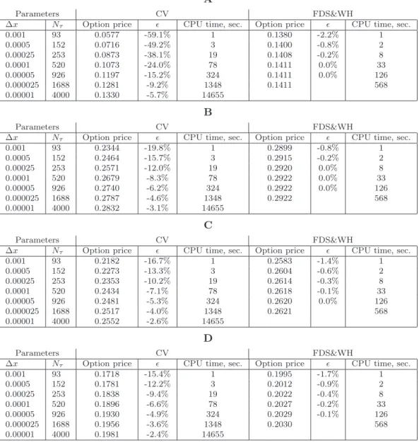
In this subsection we apply our finite difference scheme with Wiener-Hopf method (we refer to the method FDS&WH) to KoBoL process, and com-pare barrier option prices with the results obtained by the method in Cont– Voltchkova (2005) [15] (we refer to this method as CV method). We study convergence of two methods for processes of order ν <1 and ν > 1.
Example 1. Process of order ν < 1. To compare CV-method with FDS&WH for processes of order ν <1, we take KoBoL model with parame-ters σ= 0, ν = 0.5, λ+ = 4.0, λ−=−6.0,c= 1.0. We choose instantaneous
interest rate r= 0.04879, time to expiry T = 0.5 year, strike price K = 100
and the barrier H = 90. As the base finite difference scheme we choose the one developed in [25].
In Table 1, we compare the down-and-out barrier put option prices cal-culated by FDS&WH and CV methods for spot prices S = 91,101,111,121
1.6GHz, 896Mb, under Windows’XP). We see that FDS&WH demonstrates very fast convergence: in few seconds the accuracy reaches less than0.5%. In the same time CV-method converges very slowly and gives after several hours of calculation error in 2−3%. From the Table 1 we clearly see that prices computed by FDS&WH stabilize sufficiently fast, while the ones computed by CV-method essentially vary from the previous space step. Notice that near the barrier the prices computed by CV-method are especially unstable.
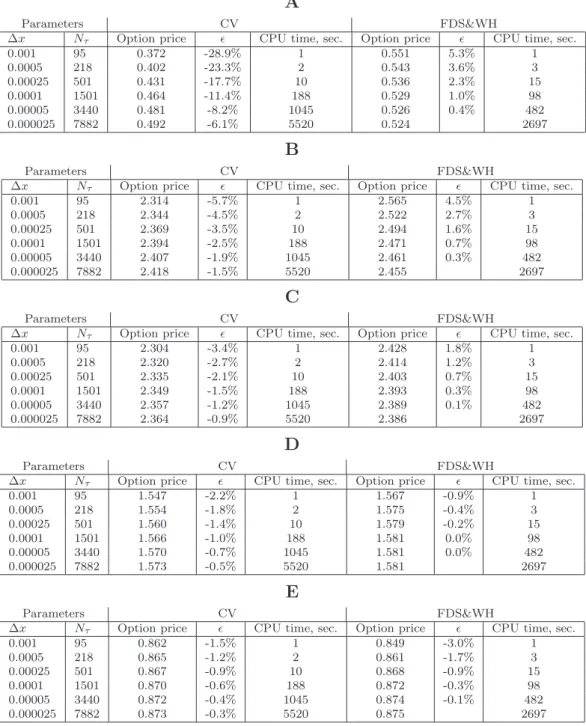
Example 2. Process of order ν >1. In the case of processes of order
ν > 1, we take KoBoL model with parameters σ = 0, ν = 1.2, λ+ = 8.8, λ− = −14.5, c = 1. We choose riskless rate r = 0.04879, time to expiry
T = 0.1 year, strike price K = 100 and the barrier H = 80.
In Table 2, we compare the down-and-out barrier put option prices cal-culated by FDS&WH and CV methods. For processes of order ν > 1 CV-method demonstrates better convergence in comparison with the previous example, but FDS&WH converges faster, especially in the neighborhood of the barrier.
6.2
FDS&WH vs. FDS
In this subsection we apply our finite difference scheme with Wiener-Hopf method to KoBoL process, and compare American option prices with the re-sults obtained by the finite difference method in [25] (we refer to this method as FDS method). We take KoBoL model with parameters σ = 0, ν = 0.2,
λ+= 3.2,λ−=−5.4, c= 1. We choose riskless rater = 0.03, time to expiry T = 0.5year, strike priceK = 100. The differences between prices and early exercise boundaries computed by the both methods are insignificant. The Table 3 confirms our observation. As we see form the Table 3 the time of computation by the FDS&WH method is in several times smaller.
7
Conclusion
Many option pricing problems can be solved by using finite difference method. The method is very popular in practice, because in a diffusion model, the correspondent system has a tridiagonal matrix which can be easily inverted. In the presence of jumps, we have the additional integral term which can be replaced by a discrete sum. As the result, one needs to invert a dense Toeplitz matrix. To avoid this problem, many authors (see e.g. [15, 13, 19]) suggest to compute the integral part by using the solution from the previous time step, while the differential term is treated implicitly. This leads to the explicit-implicit scheme, with tridiagonal system which can be
Table 1: Convergence of the down-and-out put prices in KoBoL model,ν <1: FDS&WH vs. CV
A
Parameters CV FDS&WH
∆x Nτ Option price ǫ CPU time, sec. Option price ǫ CPU time, sec.
0.001 93 0.0577 -59.1% 1 0.1380 -2.2% 1 0.0005 152 0.0716 -49.2% 3 0.1400 -0.8% 2 0.00025 253 0.0873 -38.1% 19 0.1408 -0.2% 8 0.0001 520 0.1073 -24.0% 78 0.1411 0.0% 33 0.00005 926 0.1197 -15.2% 324 0.1411 0.0% 126 0.000025 1688 0.1281 -9.2% 1348 0.1411 568 0.00001 4000 0.1330 -5.7% 14655 B Parameters CV FDS&WH
∆x Nτ Option price ǫ CPU time, sec. Option price ǫ CPU time, sec.
0.001 93 0.2344 -19.8% 1 0.2899 -0.8% 1 0.0005 152 0.2464 -15.7% 3 0.2915 -0.2% 2 0.00025 253 0.2571 -12.0% 19 0.2920 0.0% 8 0.0001 520 0.2679 -8.3% 78 0.2922 0.0% 33 0.00005 926 0.2740 -6.2% 324 0.2922 0.0% 126 0.000025 1688 0.2787 -4.6% 1348 0.2922 568 0.00001 4000 0.2832 -3.1% 14655 C Parameters CV FDS&WH
∆x Nτ Option price ǫ CPU time, sec. Option price ǫ CPU time, sec.
0.001 93 0.2182 -16.7% 1 0.2583 -1.4% 1 0.0005 152 0.2273 -13.3% 3 0.2604 -0.6% 2 0.00025 253 0.2353 -10.2% 19 0.2614 -0.3% 8 0.0001 520 0.2434 -7.1% 78 0.2618 -0.1% 33 0.00005 926 0.2481 -5.3% 324 0.2620 0.0% 126 0.000025 1688 0.2517 -4.0% 1348 0.2621 568 0.00001 4000 0.2552 -2.6% 14655 D Parameters CV FDS&WH
∆x Nτ Option price ǫ CPU time, sec. Option price ǫ CPU time, sec.
0.001 93 0.1718 -15.4% 1 0.1995 -1.7% 1 0.0005 152 0.1781 -12.2% 3 0.2012 -0.9% 2 0.00025 253 0.1838 -9.4% 19 0.2022 -0.4% 8 0.0001 520 0.1896 -6.6% 78 0.2027 -0.2% 33 0.00005 926 0.1930 -4.9% 324 0.2029 -0.1% 126 0.000025 1688 0.1956 -3.6% 1348 0.2030 568 0.00001 4000 0.1981 -2.4% 14655 KoBoL parameters: σ= 0,ν= 0.5,λ+= 4,λ−=−6,c= 1.
K= 100,H= 90,r= 0.04879,T= 0.5,ǫ– the relative difference between the current option price and the price computed by FDS&WH method for space step∆x= 0,000025.
Table 2: Convergence of the down-and-out put prices in KoBoL model,ν >1: FDS&WH vs. CV
A
Parameters CV FDS&WH
∆x Nτ Option price ǫ CPU time, sec. Option price ǫ CPU time, sec.
0.001 95 0.372 -28.9% 1 0.551 5.3% 1 0.0005 218 0.402 -23.3% 2 0.543 3.6% 3 0.00025 501 0.431 -17.7% 10 0.536 2.3% 15 0.0001 1501 0.464 -11.4% 188 0.529 1.0% 98 0.00005 3440 0.481 -8.2% 1045 0.526 0.4% 482 0.000025 7882 0.492 -6.1% 5520 0.524 2697 B Parameters CV FDS&WH
∆x Nτ Option price ǫ CPU time, sec. Option price ǫ CPU time, sec.
0.001 95 2.314 -5.7% 1 2.565 4.5% 1 0.0005 218 2.344 -4.5% 2 2.522 2.7% 3 0.00025 501 2.369 -3.5% 10 2.494 1.6% 15 0.0001 1501 2.394 -2.5% 188 2.471 0.7% 98 0.00005 3440 2.407 -1.9% 1045 2.461 0.3% 482 0.000025 7882 2.418 -1.5% 5520 2.455 2697 C Parameters CV FDS&WH
∆x Nτ Option price ǫ CPU time, sec. Option price ǫ CPU time, sec.
0.001 95 2.304 -3.4% 1 2.428 1.8% 1 0.0005 218 2.320 -2.7% 2 2.414 1.2% 3 0.00025 501 2.335 -2.1% 10 2.403 0.7% 15 0.0001 1501 2.349 -1.5% 188 2.393 0.3% 98 0.00005 3440 2.357 -1.2% 1045 2.389 0.1% 482 0.000025 7882 2.364 -0.9% 5520 2.386 2697 D Parameters CV FDS&WH
∆x Nτ Option price ǫ CPU time, sec. Option price ǫ CPU time, sec.
0.001 95 1.547 -2.2% 1 1.567 -0.9% 1 0.0005 218 1.554 -1.8% 2 1.575 -0.4% 3 0.00025 501 1.560 -1.4% 10 1.579 -0.2% 15 0.0001 1501 1.566 -1.0% 188 1.581 0.0% 98 0.00005 3440 1.570 -0.7% 1045 1.581 0.0% 482 0.000025 7882 1.573 -0.5% 5520 1.581 2697 E Parameters CV FDS&WH
∆x Nτ Option price ǫ CPU time, sec. Option price ǫ CPU time, sec.
0.001 95 0.862 -1.5% 1 0.849 -3.0% 1 0.0005 218 0.865 -1.2% 2 0.861 -1.7% 3 0.00025 501 0.867 -0.9% 10 0.868 -0.9% 15 0.0001 1501 0.870 -0.6% 188 0.872 -0.3% 98 0.00005 3440 0.872 -0.4% 1045 0.874 -0.1% 482 0.000025 7882 0.873 -0.3% 5520 0.875 2697 KoBoL parameters: σ= 0,ν= 1.2,λ+= 8.8,λ−=−14.5,c= 1.
K= 100,H= 80,r= 0.04879,T= 0.1;Nτ – number of time steps;ǫ– the relative difference between
the current option price and the price computed by FDS&WH method for space step∆x= 0.000025. Panel A:S= 81; Panel B:S= 91; Panel C:S= 101; Panel D:S= 111; Panel E:S= 121.
Table 3: American put, time of computation: FDS&WH vs. FDS
Parameters Relative difference Time of computation, sec. Space step∆x Number of time stepsNτ ǫp ǫb FDS FDS&WH
0.002 65 0.21% 0.2% 14 1
0.001 112 0.21% 0.2% 64 3
0.0005 203 0.2% 0.2% 536 13 KoBoL parameters: σ= 0,ν = 0.2,λ+= 3.2,λ−=−5.4,c= 1.
K= 100,r= 0.03,T = 0.5.
ǫp andǫbare the maximums of the relative differences between correspondent prices and
boundaries, respectively, in the regionS≤1.3K.
solved inO(MlnM)operations, whereM is a number of space discretization points. However, the advantage in speed turns to the drawback in accuracy, especially in the case of barrier options. In the infinite activity case described in [15], the explicit-implicit scheme demonstrates bad convergence near the barrier and hence also becomes time consuming (see details in [23]).
In [25], an accurate implicit finite difference scheme for pricing American options was developed. The procedure of inversion for the dense matrix of the system is iterative, and it requires 5–10 iterations on each time step. Hence, for a fixed space and time steps modification of the scheme for barrier options is in several times slower than than the scheme in [15], but more accurate as examples in [23] show.
In [18], the case of discrete monitoring is considered. The usual backward recursion that arises in discrete barrier option pricing is converted into a set of independent integral equations by using a z-transform approach. In order to solve these equations, the rectangle quadrature rule transforms each integral equation into a Toeplitz linear system which is solved by iterative algorithms as in [25].
In the paper, we suggest a new approach which incorporates the Wiener-Hopf factorization method into a finite difference scheme with a Toeplitz system. Notice that our algorithm has the same complexity as the ones which use the explicit-implicit scheme, with a tridiagonal matrix. However, our method is more accurate, because it inverts the whole Toeplitz matrix, but not only its tridiagonal part.
We give an important probabilistic interpretation based on the infinitely divisible distributions theory to the Laurent operators in the Wiener-Hopf factorization identity for finite difference schemes. It implies very useful properties which allow to develop effective methods for solving many stan-dard problems on option pricing (e.g. European, barrier, first touch digital
and American options).
A
Formulas for the coefficients
α
k,
the case of KoBoL,
ν >
1
Let the Le´vy densities of negative and positive jumps F∓(dx) are given by (2.8). Then F∓(dx) satisfies (5.3)–(5.13) with
c+=c−=c, p+(x) =ceλ−x, p−(x) =ceλ+x.
Introduce the following notations.
(α)0 = 1, (α)m = α·(α+ 1)·...·(α+m−1), m= 1,2, ...; bn(l, ǫ, ν) = n X m=0 Cm n(ν)mǫn−m (l+ 1)m ; en(ǫ) = n X k=0 ǫk k!.
By using integration by parts, we obtain the following formulas for ˆc+l
and cˆ−l (see (5.17) and (5.31)).
ˆ c+0 = c ν +∞ X n=0 (λ−∆x)n n!(n+ 1−ν/2), (A.1) ˆ c−0 = c ν +∞ X n=0 (−λ+∆x)n n!(n+ 1−ν/2), (A.2) ˆ c+l = cexp(λ−(l+ 1)∆x) ν(l+ 1)ν +∞ X n=0 bn(l,−λ−∆x, ν) (ν/2 + 1)n+1 , l > 0, (A.3) ˆ c−l = cexp(−λ+(l+ 1)∆x) ν(l+ 1)ν +∞ X n=0 bn(l, λ+∆x, ν) (ν/2 + 1)n+1 , l > 0. (A.4) By using decomposition to the series of incomplete gamma functions, we
obtain the formulas for cˆ++l and cˆ−−l (see (5.18) and (5.32)). ˆ c++l = c ν(l+ 1)ν−1 +∞ X n=0 (λ−∆x(l+ 1))n n!(n+ 1−ν) · 1− l l+ 1 n+1−ν , 0< l≤ 2 −λ−∆x; ˆ c−−l = c ν(l+ 1)ν−1 +∞ X n=0 (−λ+∆x(l+ 1))n n!(n+ 1−ν) · 1− l l+ 1 n+1−ν , 0< l≤ 2 λ+∆x ; ˆ c++l = ce λ−∆xl νλ−∆xlν +∞ X n=0 (ν)n(eλ−∆xen(−λ−∆x)−1) (λ−∆xl)n , l > 2 −λ−∆x, ˆ c−−l = ce −λ+∆xl νλ+∆xlν +∞ X n=0 (ν)n(1−e−λ+∆xen(λ+∆x)) (−λ+∆xl)n , l > 2 λ+∆x .
Analogously, we findc+l ,c++l andc−l ,c−−l (see (5.24),(5.25) and (5.37),(5.38)). Then a bit of algebra leads us to the formulas for βl (see (5.28),(5.29) and
(5.41), (5.42),(5.45)). βl = c(−λ−) νlν−2 +∞ X n=0 (λ−∆xl) n((1 + 1/l)n+2−ν+ (1−1/l)n+2−ν−2) n!(n+ 1−ν)(n+ 2−ν) , 0< l≤ 2 −λ−∆x ; β−l = cλ+ νlν−2 +∞ X n=0 (−λ+∆xl)n((1 + 1/l)n+2 −ν+ (1−1/l)n+2−ν−2) n!(n+ 1−ν)(n+ 2−ν) , 0< l≤ 2 λ+∆x ; βl = ceλ−∆xl ν∆xlν−1 +∞ X n=1 (ν)n−1 (λ−∆xl)n h n(2−eλ−∆xe n(−λ−∆x)−e −λ−∆xe n(λ−∆x)) + λ−∆x(e −λ −∆xe n−1(λ−∆x)−e λ−∆x en−1(−λ−∆x)) i , l > 2 −λ−∆x , β−l = ce−λ+∆xl ν∆xlν−1 +∞ X n=1 (ν)n−1 (−λ+∆xl)n h n(2−e−λ+∆xe n(λ+∆x)−eλ+∆xen(−λ+∆x)) − λ+∆x(eλ+∆xen−1(−λ+∆x)−e−λ+∆xen−1(λ+∆x)) i , l > 2 λ+∆x .
gamma functions.
C+ = cΓ(−ν)((−λ−)ν−1(−λ−−1)−(−λ−−1)ν); (A.5) C− = cΓ(−ν)(λν−1
+ (λ++ 1)−(λ++ 1)ν). (A.6)
Then we find γl by using the formulas (5.21)(5.22) and (5.35),(5.36),
(5.44).
Finally, we define the drift by (5.47), and find coefficients αl by the
for-mulas (5.52)-(5.54)
References
[1] Amin, K., 1993, “Jump-diffusion option valuation in discrete time", J. Finance, 48, 1833-1863.
[2] Barndorff-Nielsen, O. E., 1998, “Processes of Normal Inverse Gaussian Type", Finance and Stochastics, 2, 41–68.
[3] Barndorff-Nielsen, O. E., and S. Levendorskiˇi, 2001, “Feller Processes of Normal Inverse Gaussian type", Quantitative Finance, 1, 318–331. [4] Boyarchenko, M. and S. Boyarchenko (2011) : “Double Barrier Options
in Regime-Switching Hyper-Exponential Jump-Diffusion Models”, to appear in International Journal of Theoretical and Applied Finance. Available at SSRN: http://ssrn.com/abstract=1440332
[5] Boyarchenko, S. I., and S. Z. Levendorskiˇi, (1999) “Generalizations of the Black-Scholes equation for truncated Lévy processes", Working Paper, University of Pennsylvania, Philadelphia.
[6] Boyarchenko, S. I., and S. Z. Levendorskiˇi, 2000, “Option pricing for truncated Lévy processes", International Journal of Theoretical and Applied Finance, 3, 549–552.
[7] Boyarchenko, S. I., and S. Z. Levendorskiˇi, (2002) Non-Gaussian Merton-Black-Scholes theory, World Scientific, New Jercey, London, Singapore, Hong Kong.
[8] Boyarchenko S.I. and S.Z. Levendorskiˇi (2005): “American options: the EPV pricing model", Annals of Finance, 1:3, 267–292.
[9] Boyarchenko, S. I., and S.Z. Levendorskiˇi (2007) : Irreversible Deci-sions under Uncertainty (Optimal Stopping Made Easy). Series: Stud-ies in Economic Theory, Vol. 27, Berlin: Springer-Verlag.
[10] B¨ottcer, A., and B. Silbermann, (1999)Introduction to large truncated Toeplitz matrices, Springer-Verlag, New York, Berlin, Heidelberg. [11] Carr, P., (1998) “Randomization and the American put", Review of
Financial Studies, 11, 597-626.
[12] Carr, P., H. Geman, D.B. Madan, and M. Yor, (2002) “The fine struc-ture of asset returns: an empirical investigation", Journal of Business, 75, 305-332.
[13] Carr, P., and A. Hirsa, (2003) “Why be backward?",RiskJanuary 2003, 26, 103–107.
[14] Cont, R., and P.Tankov, (2004) Financial modelling with jump pro-cesses, Chapman & Hall/CRC Press.
[15] Cont, R., and E. Voltchkova, (2005) “A finite difference scheme for option pricing in jump diffusion and exponential Lévy models.", SIAM Journal on Numerical Analysis, 43, No. 4, 1596–1626.
[16] Eberlein, E., and U. Keller, (1995) “Hyperbolic distributions in fi-nance", Bernoulli, 1, 281–299.
[17] Eberlein, E., U. Keller and K. Prause, (1998) “New insights into smile, mispricing and value at risk: The hyperbolic model", Journal of Busi-ness, 71, 371–406.
[18] Fusai, G., Marazzina, D., Marena, M. and Ng, M. (2011) “Z-Transform and preconditioning techniques for option pricing”, Quantitative Fi-nance, First published on: 15 April 2011 (iFirst)
[19] Hirsa, A., and D.B. Madan, (2003) “Pricing American options under Variance Gamma”,Journal of Computational Finance, 7:2.
[20] Koponen, I. (1995) : “Analytic approach to the problem of conver-gence of truncated Lévy flights towards the Gaussian stochastic pro-cess”, Physics Review E, 52, 1197–1199.
[21] Kou, S.G. (2002) : “A jump-diffusion model for option pricing”. Man-agement Science, 48, 1086–1101.
[22] Kou, S.G.(2008): Discrete barrier and lookback options. In: Birge, J.R., Linetsky, V. (eds.) Financial Engineering. Handbooks in Oper-ations Research and Management Science, vol. 15, 343–373. Elsevier, Amsterdam.
[23] Kudryavtsev, O., and S. Levendorskiˇi (2009) : “Fast and accurate pric-ing of barrier options under Levy processes”. J. Finance Stoch., 13(4), 531–562.
[24] Levendorskiˇi, S.Z., (2004) “Pricing of the American put under Lévy processes", International Journal of Theoretical and Applied Finance, 7, 303–335.
[25] Levendorskii, S., Kudryavtsev, O., and V.Zherder, (2006) “The relative efficiency of numerical methods for pricing American options under Lévy processes”, Journal of Computational Finance, Vol. 9. No 2. [26] Lipton, A., (2002) “Assets with jumps”, Risk (September 2002) 149–
153.
[27] Lukacs, E., (1960)Characteristic functions. Charles Griffin & Company limited, London.
[28] Merton, R. (1976) “Option pricing when underlying stock returns are discontinuous”. J. Financ. Econ. 3, 125–144
[29] Madan, D.B., Carr, P., and E. C. Chang (1998) “The variance Gamma process and option pricing”, European Finance Review, 2, 79–105. [30] Matache, A. M., Nitsche, P. A., and C. Schwab, 2005, “Wavelet
Galerkin Pricing of American Options on Lévy Driven Assets”, Quan-titative Finance, Vol. 5, No 4, 403–424.
[31] Press,W., Flannery,B., Teukolsky, S. and W. Vetterling, 1992, Numer-ical recipes in C: The Art of Scientific Computing, Cambridge Univ. Press, available at www.nr.com.
[32] Sato, K., 1999, Lévy processes and infinitely divisible distributions, Cambridge University Press, Cambridge.
[33] Schoutens, W. (2006): “Exotic options under Lévy models: An overview”. J. Comput. Appl. Math., 189, 526–538.
PARIS - ROCQUENCOURT BP 105 - 78153 Le Chesnay Cedex inria.fr