Insider information and its relation with the arbitrage condition and the utility maximization problem

Working paper

2019-11

ISSN 2387-0303

Insider information and its relation with

the arbitrage condition and the

utility maximization problem

%HUQDUGR'¶$XULD-RVp$QWRQLR6DOPHUyQ

Serie disponible en http://hdl.handle.net/10016/12

Creative Commons Reconocimiento-NoComercial- SinObraDerivada 3.0 España (CC BY-NC-ND 3.0 ES)

Insider information and its relation with the arbitrage

condition and the utility maximization problem

Bernardo D’Auria

Jos´

e Antonio Salmer´

on

September 12, 2019

Abstract

Within the well-known framework of financial portfolio optimization, we ana-lyze the existing relationships between the condition of arbitrage and the utility maximization in presence of insider information. That is, we assume that, since the initial time, the information flow is altered by adding the knowledge of an ad-ditional random variable including future information. In this context we study the utility maximization problem under the logarithmic and the Constant Relative Risk Aversion (CRRA) utilities, with and without the restriction of no temporary-bankruptcy. For the latter case we obtain an optimal strategy different from the one computed in [1]. We give various examples for which the insider information create arbitrage, and for which the logarithmic maximization problem is bounded or unbounded. We conclude with an interesting result, showing that the insider information may not lead to any arbitrage.

Keywords— Optimal portfolio, Enlargement of filtration, Value of the information, Ar-bitrage, No Free Lunch Vanishing Risk, Equivalent Martingale Measure.

1

Introduction

In the field of financial mathematics, the problem of the optimal portfolio plays a crucial role and in recent years it has been deeply analyzed in the literature. In its simplest form it consists in finding the best strategy in order to maximize a given utility function at a fixed terminal finite time.

In the simplified settings of just two assets, one risk-less and one risky, the optimal portfolio problem has been introduced and solved in [2] by considering both the logarithmic and risk adverse utilities. Later, a more general model was considered in [3].

∗_{This research was partially supported by the Spanish Ministry of Economy and}

Competitive-ness Grants MTM2017-85618-P via FEDER funds and MTM2015-72907-EXP; both authors thank the NYUAD, Abu Dhabi (United Arab Emirates) for hosting them during the fall 2018.

†_{UC3M, Department of Statistics, 28911, Legan´es, Spain & UC3M-BS, Institute of Financial Big}

Data, 28903 Getafe, Spain ([email protected]).

‡_{This author acknowledges financial support by an FPU Grant (FPU18/01101) of Spanish Ministerio}

de Ciencia, Innovaci´on y Universidades.

§_{UC3M, Department of Statistics, 28911, Legan´es, Spain ([email protected]).}

1 INTRODUCTION 4

One fundamental ingredient in computing the optimal portfolio is the information flow that the agent employs in order to build her strategy. The information flow is modeled mathemat-ically by the concept of filtration, and the restrictions on the agent choices are modeled by requiring that her portfolio is adapted to this filtration. While in general the underlying filtra-tion is the one naturally generated by the set of risky assets, in the literature the interest has recently grown about analyzing filtrations that contain additional information.

The technique consisting in substituting the natural filtration by a larger one containing additional information, is generally referred to as enlargement of filtration and has been intro-duced and studied in the seminal works [4, 5, 6, 7]. The concept of enlargement of filtration was first applied to the financial setting by the seminal work [1], to describe situations in which the agent has access to privileged information and to model the insider trading portfolios. Also [8], in which a statistical test to detect if an agent is playing with the insider strategy or not is proposed.

In [1], various examples of initial enlargements were analyzed by computing the expected additional gain carried by the privileged information. It was shown that the knowledge of the price of the stock at a given moment in the future, implies an expected unbounded additional profit while the knowledge of an interval of values containing the future price only added a bounded expected additional gain. For the case of an infinite interval, a direct proof of this result was given in [1] while, for the case of a finite interval, the result was only conjectured by the support of numerical calculations. Later a series of remarkable works, [9, 10], employed the concept of theFischer Entropy Theory, shortly mentioned already in [1], to close the conjecture. In Theorem 4.15 below we prove again this result by the same techniques used in [1]. In [11], the Fischer Entropy Theory is generalized for a more broad class of enlargement filtration.

In more recent years many results on insider trading models appeared, we just mention [12, 13, 14, 15] and references therein.

The above research indicates that there should exist a relation between the type of additional information, such as if it is exact or it is of interval type, and the value that it carries in terms of its contribution to the maximal expected utility. A partial result to this question has been given in [9] where they look at the atomicity of the insider information. However there are many questions still open, for example to understand if the value of the information is bounded or not according to the fact that it introduces an arbitrage in the financial model.

On this direction, [16] analyzes the relation between the arbitrage condition – in particu-lar the (NFLVR), see Proposition 2.11 below – and the integrability of the drift of the semi-martingale representation of the asset in the enlarged filtration, see Proposition 2.9 below. Also, the works [17, 18, 19] studied the relation of a weak arbitrage condition, the No Unbounded Profits with Bounded Risk property (NUPBR) with the initial enlargement of filtration.

It seems that an important ingredient in the analysis is the role played by the set of strategies that are allowed to be used. For example, the strategy constructed in [1] to play with the information given by an interval of future prices, does not take advantage of the arbitrage condition introduced by this information. This is due to the fact that the proposed strategy avoids the possibility for the insider agent to be for some moments in time in bankruptcy, what we later refer to astemporary-bankruptcy. However it is possible to construct, by removing this constraint, even simpler strategies that get advantage of the arbitrage condition and assure a positive gain, see for example Propositions 4.7 and 4.10 below, for the semi-infinite and the finite interval respectively.

In the current work, we analyze the relations that may exist between the condition of arbitrage and the utility maximization problem under the special setting of enlargement of filtration. We first study the condition of (NFLVR), introduced in [20], and its relationship with bankruptcy, by concluding that if the privileged information implies arbitrage, the investor can improve her profit expectations by employing strategies that allow temporary-bankruptcy.

2 BASIC NOTIONS AND PRELIMINARIES 5

Even if it may seem anti-intuitive, the privileged information guarantees that the trend will be corrected and the condition of bankruptcy will be only temporary. In the examples included below, we show that optimal strategies that maximize the utility do not assure positive profits almost surely, while one can construct other strategies that, although not optimal, satisfy this condition.

In addition we prove that the insider information does not always imply arbitrage, by constructing a counter example in Section 4.3. We verify that the introduction of the privileged information does not violate the Novikov condition, Equation (2.4) below, therefore assuring the existence of an equivalent martingale measure and therefore the absence of arbitrage.

In Section 2, we provide the notation as well as the basic and preliminary notions that we adopt for the rest of the paper. It includes a more precise definition of the general framework in which the problem of the optimal portfolio is framed, such as the definition of arbitrage and the concept of enlargements of filtration. In Section 3, we introduce the utility maximization problem, analyzing it under different conditions on the set of allowed strategies, such as the no-temporary-bankruptcy, and linking it with the arbitrage conditions. Section 4 provides three examples that show various cases of enlargement of filtration, where the arbitrage condition is analyzed and the utility maximization problem is solved. Section 5 ends with some conclusions.

2

Basic notions and preliminaries

As a general setup we assume to work in a probability space (Ω,F,F,P) where F is the

event sigma-algebra, and F = {Ft, t ≥ 0} is a right continuous filtration satisfying the usual

conditions. We consider a financial market with a continuous R2 semi-martingale S = (D, S)

and, unless otherwise specified, the filtration F that is the natural one generated by S. Each

component represents the prices of an asset in which the agent could invest. Usually, the first one is assumed to be a risk-less asset driven by some interest rater >0, and the second one is given by a diffusion process whose coefficients µ and σ are processesF-adapted. According to

the following stochastic differential equations,

dDt=Dtrdt, D0 = 1. (2.1a)

dSt=µ(t, St)dt+σ(t, St)dBt , (2.1b)

where the processB = (Bt,0≤t≤T) is a standard Brownian motion in the filtration F. We

fixT >0 as a horizon time, assumed to be finite. The semi-martingale assumption implies that the stochastic integral operator is well defined. So, for anR2 valued predictable andF-adapted

process H = (H1, H2), we use the notation (H· S)t to denote the sum of the components of

the Itˆo integral, i.e.

(H· S)t= ∫ t 0 H_u1dDu+ ∫ t 0 H_u2dSu t∈[0, T]. (2.2)

We refer to the process D−1S = (1, D−1S) as the discounted price process. We define the process Θ = {(Mt, Nt) : 0 ≤ t ≤ T} as the number of shares that the agent owns of each

asset at any timet∈[0, T]. Assuming that, in the market, short-selling and borrowing money from the bank is allowed, there is no restriction on the values assumed by the process Θ. To guarantee the existence of the Itˆo integral (Θ· S)T, we are going to work with a restricted class

of strategies, the one satisfying the following definition.

Definition 2.1. Given the filtrationT={Tt, t≥0}, we define an allowed portfolioprocess as a

progressiveT_t-measurable process ΘT_{(t, ω) : [0, T]×Ω−→R}2_{which satisfies}∫T

0 ∥ΘTtσ(t, St)∥2dt <

2 BASIC NOTIONS AND PRELIMINARIES 6

The total wealth of anallowed portfolioprocess Θ is then defined as the following Itˆo integral

X_tΘ=MtDt+NtSt (2.3a)

=X0+ (Θ· S)t t∈[0, T]. (2.3b)

The second equality indicates that Θ satisfies theself-financing condition.

2.1

Classical arbitrage conditions

In this section we are going to define the concepts of arbitrage with the special care of denoting the set of strategies that the agent is restricted to use. We do so by explicitly including in the definition of the arbitrage conditions the set of allowed strategies. In the following we use the notation A(T) to denote a general set of T-progressive admissible strategies, later we will

replace it with more concrete examples. Again when T=F, we omit to indicate the filtration

in the notation.

For the following, we need some technical definitions. We refer toL∞(Ω,FT,P) as the set of F_T-measurable bounded random variables, equipped with the essential supremum norm∥X∥∞.

We abbreviate it to L∞ when the measure P is established. Finally we use L∞₊(Ω,FT,P) to

denote the class of non-negative FT-measurable bounded random variables and L0+(Ω,FT,P)

for the class ofF_T-measurable positive random variables.

Following the classical definition in [21, Definition 2.8], we definethe set of contingent claims

A-attainable at price 0, K(A) = { (Θ· S)T|Θ∈ A } ={X_TΘ−X0|Θ∈ A} .

This set contains all possible random values of terminal wealth that an agent with initial 0 wealth can reach at time T by only applying A-admissible strategies. Then, by allowing the possibility of “throwing away money” at timeT, we define the sets

C0(A) =K(A)−L0+ ={(Θ· S)T −f |Θ∈ A, f ≥0 finite},

C(A) =C0(A)∩L∞.

together with the set C(A) as the closure ofC(A) inL∞.

Given the above, we are ready to state the most important definition in Arbitrage Theory. A complete review of this theory is given in [22].

Definition 2.2. Given a semi-martingale S and a set of admissible strategiesA we say that (N A)A: the condition of No Arbitrage holds on A when K(A)∩L∞+ ={0}.

(N F LV R)A: the condition of No Free Lunch with Vanishing Riskholds on AwhenC(A)∩L∞+ ={0}.

We also define the conditions of Arbitrage, (A)A, and Free Lunch with Vanishing Risk,

(F LV R)A, as the complements of the conditions above, that is (N A)A and (N F LV R)A

re-spectively.

Since K(A)⊂C(A), it immediately follows that (NFLVR) implies (NA).

With the following definitions, we describe the main sets of strategies that an agent is allowed to use. The reason to consider different sets of strategies is mainly due to the fact that some of them allow the agent to have negative total wealth for some moments in time – condition that we refer to astemporary-bankruptcy –, while others do not allow for this possibility.

2 BASIC NOTIONS AND PRELIMINARIES 7

Definition 2.3. An allowed portfolio processΘ is called a-admissible, with a >0, if(Θ· S)t≥ −a, ∀t ∈[0, T] almost surely. If last inequality is strict we call Θ super a-admissible, and we simply call it admissible if it is a-admissible for some a >0.

Definition 2.4. The set of all admissible (resp. a-admissible) strategies is denoted byH (resp.

Ha). We write H∗a for the set of supera-admissible strategies. In particular, we use H+ for the

set H∗

X0.

In the following, we will mainly work with the setH andH+_{, the latter being the one that}

forbids the condition of temporary-bankruptcy.

Although the concepts of (NA) and (NFLVR) have been introduced, as above, from a functional analysis point of view both have strong implications in a strictly financial framework. The following classical results, for the case A=H, give a characterization of the (NFLVR) in terms of agent’s wealth. It refers to the possibility of approximating an arbitrage opportunity by reducing the risk as close to zero as wanted. The following statement appears in [21, Corollary 3.7].

Proposition 2.5. The(F LV R)Hholds if and only if there exists a sequence(Θn)∞n=1⊂ H and

a non negative random variable, by a slight abuse of notation denoted by (Θ∞· S)T, such that

P((Θ∞· S)T >0)>0, (Θn· S)T →(Θ∞· S)T almost surely and∥(Θn· S)_T−∥∞→0 asn→ ∞.

In the following we recall the central result of the theory of pricing and hedging by no-arbitrage, that relates the condition of no arbitrage with the existence of an Equivalent Mar-tingale Measure (ELMM). A proof of this result, known as the Fundamental Theorem of Asset Pricing, is given in quite general settings in [21].

Definition 2.6. The semi-martingale S satisfies (ELMM) if there is a probability measure Q

onF equivalent to P such that the discounted price process is a local martingale with respect to (Ω,F,Q).

Proposition 2.7 (Fundamental Theorem of Asset Pricing). The semi-martingale S satisfies (N F LV R)H if and only if it satisfies (ELMM).

The following result on change of probabilities provides a necessary condition for the exis-tence of an ELMM and it will be useful in the context of enlargements of filtration introduced in the next section.

Proposition 2.8 (Cameron-Martin-Girsanov). Let θ = (θt,0 ≤ t ≤ T) be an F predictable

process such that

E [ exp ( 1 2 ∫ T 0 θ2_tdt )] <+∞ (Novikov’s Condition) , (2.4) then there exists a measure Q on(Ω,FT), equivalent toP, such that

dQ dP =E ( − ∫ T 0 θtdBt ) and Wt=Bt+ ∫t 0θuduis a (F,Q) Brownian motion.

2 BASIC NOTIONS AND PRELIMINARIES 8

2.2

Enlargement of filtrations

In this section we introduce the concepts required to model the portfolio of an insider agent. We assume that an insider has at her disposal more information than the one freely accessible, and we model this by enlarging the filtration with respect to which she can look for adapted strategies.

To this end, we introduce the filtration G={Gt, t≥0} that we assume larger than F, that

isF⊂G. In particular we focus on the case where the additional information is accessible since

the initial time, that is

Gt=Ft∨σ(G) , (2.5)

whereG∈ FT is a real random variable modeling the privileged information.

In order to assure that anyFsemi-martingale is also aGsemi-martingale, what is known in

the literature ashypothesis (H’), see [4], for the rest of this paper we assume that the following equivalent hypothesis holds. This is thecondition (A) appearing in [5], where it is also proved its equivalence to the hypothesis (H’).

Assumption: The distribution ofGis positive andσ-finite while the regularF_t-conditional distributions almost surely verifies for t ∈ [0, T) the absolutely continuity condition P(G ∈ ·|Ft)≪P(G∈ ·).

The above assumption assures the existence of a jointly measurable process ηg = (ηg_t,0≤

t≤T), with (g, t)∈R×[0, T] such that P(A) =∫_AηgtP(G∈dg) for any A∈ Ft.

The following result allows to compute the G-semi-martingale decomposition of an F

-semi-martingale. Its proof is given in [5].

Proposition 2.9(Jacod, 1985). There exists a jointly measurable processαg = (α_tg,0≤t≤T), with (g, t)∈_R×[0, T] such that,

• ∫t 0(α g u)2du <+∞ almost surely on σ(G). • ⟨ηG, B⟩t= ∫t 0 η G uαGudu. and Wt=Bt− ∫t 0α G udu is a G-Brownian motion.

Remark 2.10. Using the second statement of the previous lemma, we can write

η_tG=E ( − ∫ t 0 αG_udBu ) ,

where E(X) denotes the Dol´eans-Dade exponential of the semi-martingaleX, see also [7, 23]. The following proposition gives a first relation between the (FLVR) arbitrage condition and theαG _{process. For a proof see [16].}

Proposition 2.11. If P(∫T 0 (α G t)2dt=∞ ) >0, then S satisfies (F LV R)H(G).

Using results from the previous section combined with the semi-martingale decomposition given in Proposition 2.9 we can construct a simple test to check the (NFLVR)H(G) condition in

presence of initial enlargement of filtration.

Corollary 2.12. Let G as in (2.5), if the processαG= (αG_t ,0≤t≤T) satisfies

E [ exp ( 1 2 ∫ T 0 (αG_t)2dt )] <+∞ , (2.6) then(N F LV R)H(G) holds true.

Proof. By the Fundamental Theorem of Asset Pricing, Proposition 2.7, the NFLVR condi-tion follows by the existence of an ELMM. Combining the Cameron-Martin-Girsanov theorem, Proposition 2.8 with the semi-martingale decomposition given in Proposition 2.9, this follows by condition (2.6) that in this context is equivalent to the Novikov condition (2.4).

3 UTILITY MAXIMIZATION PROBLEM 9

3

Utility maximization problem

In this section we begin to study the relationships between the set of strategy that the agent is allowed to employ with her maximum expected profit and in general with the conditions of arbitrage. We start by introducing the general class of utility functions, and then by considering the associated maximal expected utility. The utility functions are chosen to satisfy the classical assumptions, that is to be increasing, continuous, differentiable and strictly concave. These assumptions have perfect sense economically.

Definition 3.1. Let T = {Tt, t ≥ 0} be a given filtration and Uγ(x) = (xγ −1)/γ+γ, with

γ ∈(0,1), an utility function, we denote by

vT γ(A) = sup Θ∈A(T) E[Uγ(XTΘ) ] γ ∈(0,1) ,

the corresponding maximal expected utility of the agent constrained to work with the strategies belonging to the set A. For the extreme cases we use the notations uT_{(A) := lim}

γ→0vγT(A) and

vT_{(A) = lim}

γ→1vγT(A). Following the convention adopted above, we omit in the notation to

include the filtration T whenever the underlying one isF.

Remark 3.2. The utility functions as introduced above are a slight modification of the classical Constant Relative Risk Aversion (CRRA) functions, see [2, 24], by the additional constant term

γ. We use this modified form as they preserve the same optimal portfolio while including the improper linear utility function forγ = 1.

Proposition 3.3. With the previous notation, the following inequalities hold,

uT_(H+_{)< v}T

γ(H+)< vT(H+)≤vT(H)

Proof. The first two inequalities follow by the fact that Uγ(x) is strictly increasing in the

parameterγ while the last one by the fact that H+_{⊂ H.}

If the agent plays with the strategy setH+_{, the evolution of the capital can be reformulated}

as follows, dX_tΘ=MtdDt+NtdSt⇐⇒ dX_tΘ XΘ t = MtDt XΘ t dDt Dt +NtSt XΘ t dSt St = (1−πt) dDt Dt +πt dSt St , (3.1) beingπ= (πt,0≤t≤T) the proportion of wealth invested in the risky asset, satisfying the

integrability condition. This change does not alter the dynamic ofXtbecause we are assuming {Xt>0} almost surely in ω∈Ω and ∀t∈[0, T]. We conclude that both models are identical

only when the agent restricts herself to use H+ _{strategies. In the examples of the following}

section, we will use this model.

In the following result we show that, with a sufficiently large initial capital, arbitrage op-portunities do not depend on the bankruptcy.

Lemma 3.4. Given a filtration T, the following equivalence hold

(N A)H(T)⇐⇒ {(N A)H+(T), ∀X0∈R+} .

Proof. The necessary condition follows from the inclusionH+ _{⊂ H. For the sufficient one, let}

us assume that (N A)H+₍

T) holds true for all X0 ∈ R

+_{. If (A)}

H(T) holds, then there exists a

strategy Θ ∈ H(T) such that (Θ· S)T ≥ 0 almost surely with P((Θ· S)T > 0) > 0. From

the fact that Θ ∈ H(T) we deduce that there exists a constant a > 0 such that, ∀ t ∈ [0, T],

(Θ· S)t≥ −a almost surely. So considering the portfolioXt=a+ (Θ· S)t, we see that we get

XT ≥aalmost surely withP(XT > a)>0, therefore implying that (A)H+₍

T)holds forX0=a,

4 EXAMPLES 10

We present a technical result that we will use later. A proof of this result is given in [16].

Lemma 3.5. LetS = (D, S)be the pair of continuous semi-martingale satisfying(N F LV R)H(T).

If (Θ· S)T ≥ −X0 almost surely withΘ allowed, then the process Θ∈ H+.

Finally, we get to the result that relates the condition of (NFLVR)H(T) with the expected

terminal utility underH+₍

T) and H(T).

Proposition 3.6. LetU be an utility function suchsup_x∈R{U(x) =−∞}= 0, then the

follow-ing implications hold.

(N F LV R)H(T)=⇒ sup Θ∈H(T) E[U(X_TΘ)]= sup Θ∈H+₍ T) E[U(X_TΘ)].

Proof. We assume there exists Θ∈ HthatE[U(X_TΘ)]>sup_Θ∈H+₍

T)E [

U(X_TΘ)]. Then, Θ̸∈ H+

and X_tΘ ̸≥ 0 almost surely for some t ∈[0, T]. Like (NFLVR)H(T) holds, lemma 3.5 says that X_TΘ<0 with positive probability and we conclude that E[U(X_TΘ)] =−∞ follows.

4

Examples

In this section, we show several examples to highlight the differences that may or may not exist by playing with one set of strategies or another. We focus on the following specific model, deeply studied [2, 1], in where the risky asset is given by a Geometric Brownian motion. With respect equation (2.1b), we particularize the processesµ(t, St) =ηtSt andσ(t, St) =ξtSt, i.e.

dDt=Dtr dt, (4.1a)

dSt=St (ηtdt+ξtdBt) (4.1b)

wherer >0 is the constant interest rate and the processesη= (ηt,0≤t≤T) andξ= (ξt,0≤

t ≤ T) denote the drift and the volatility of the risky asset respectively. These processes are assumed to be adapted to the natural filtration of the process B with η, ξ and 1/ξ bounded. Whenever the agent plays with Θ∈ H+_{, the wealth processX is almost surely strictly positive,}

and therefore we can use an alternative form to express the SDE (2.3b), that is

dXt Xt = (1−πt) dDt Dt +πt dSt St . (4.2)

where we usedπt=StNt/Xtand (2.3a). The following result, proved in [2] and adapted here to

our notation, gives the optimal strategies and the corresponding maximal expected utilities for the cases when the agent has no additional information (i.e. under the filtration F) and works

with the strategies that do not allow bankruptcy (i.e. in the setH+_{). For more details we refer}

the reader to [1].

Theorem 4.1 (Merton, 1969). Under the filtration F the optimal strategy is

arg sup Θ∈H+ E[Uγ(XTΘ) ] = 1 1−γ ηt−r ξ2 t γ ∈[0,1) and the maximal expected utility is given, with γ ∈[0,1), by

u(H+_{) = lnX} 0+rT + 1 2 ∫ T 0 E [ ( ηt−r ξt )2] dt logarithmic utility , (4.3a) vγ(H+) = X₀γ γ E [ exp ( γrT +1 2 γ 1−γ ∫ T 0 ( ηt−r ξt )2 dt )] + γ 2₋₁ γ CRRA utility . (4.3b)

4 EXAMPLES 11

In presence of insider information, as expected, the optimal strategies change since the agent may take advantage of the additional information she has privileged access to. The following result computes the same quantities as in Theorem 4.1 but under the initial enlarged filtrationG.

The processαG = (αG_t,0≤t≤T) appearing in the statement comes from the semi-martingale decomposition given in Proposition 2.9. The result for the logarithmic utility has been proved in [1] while the one for general CRRA utilities can be obtained by solving the corresponding HJB equation. Details can be found, for example, in [24].

Theorem 4.2. Under the filtration G the optimal strategy is

arg sup Θ∈H+₍ G) E[Uγ(XT)] = 1 1−γ ( ηt−r ξ2 t +α G t ξt ) γ ∈[0,1) and the maximal expected utility is given, with γ ∈[0,1), by

uG_(H+_{) = lnX} 0+rT + 1 2 ∫ T 0 E [ ( ηt−r ξt )2] dt+1 2 ∫ T 0 E[ (αG_t )2] dt logarithmic utility , (4.4a) vG γ(H+) = X₀γ γ E [ exp ( γrT+1 2 γ 1−γ ∫ T 0 ( ηt+αGt ξt−r ξt )2 dt )] +γ 2₋₁ γ CRRA utility . (4.4b) From the result above it follows that uG_(H+_{)<+∞ if and only if} ∫T

0 E [

(αG_t )2]dt <+∞. As it is known, for the natural filtration F, an ELMM can be found and we conclude that

NFLVRH(F)holds true. In the following result, we specify if the maximal expected utility of the

agent that plays with the filtrationF for the different utilities that we have defined is bounded

or not.

Proposition 4.3. Under the modeling assumptions (4.1), vF

γ(H+) < +∞ for 0 ≤γ < 1 and

vF_{(H) =v}F_(H+_{) = +∞.}

Proof. For 0≤γ <1 the result follows by the boundedness of the processes η and 1/ξ and the following expression vγ(H+) = X₀γ γ exp(γrT)E [ exp ( 1 2 γ 1−γ ∫ T 0 ( ηt−r ξt )2 dt )] +γ 2₋₁ γ <+∞ .

Forγ = 1, using Jensen’s inequality, we get

v(H+) = lim γ→1vγ(H +_{)≥ lim} γ→1 X₀γ γ exp ( γrT+1 2 γ 1−γE [ ∫ T 0 ( ηt−r ξt )2 dt ]) + γ 2₋₁ γ = +∞. (4.5)

4.1

Example of (A)

with

v

γ

(

H

) =

∞

for

γ

∈

[0

,

1]

Fixing G = BT, we consider the enlargement of filtration G = F⋁σ(BT). This implies that

the insider agent knows since the time t = 0 the final value BT(ω) for any ω ∈ Ω. The

semi-martingale decomposition in the filtration Gis dBt=αBtTdt+dWt, αBtT =

BT −Bt

4 EXAMPLES 12

where the process W = (Wt,0 ≤ t ≤ T) is a G-Brownian motion. Applying Itˆo calculus, if

we use logarithmic utility and the strategy set H+₍

G), equation (4.2) has the following exact

solution lnXT = lnX0+ ∫ T 0 ( r(1−πt) +ηtπt+πtξt BT −Bt T−t − 1 2π 2 tξt2 ) dt+ ∫ T 0 πtξtdWt .

By pointwise maximizing the expectation of the equation above, we get the optimal strategy

π∗_t(BT) = arg sup πt∈H+(G) E[lnXT] = ηt−r ξ2 + 1 ξt BT −Bt T−t (4.7)

that implies the following pathwise capital gain

XT =X0exp ( rT +1 2 ∫ T 0 (π∗_t(BT)ξt)2dt+ ∫ T 0 π_t∗(BT)ξtdWt ) (4.8)

Proposition 4.4. Let G=BT, then vG(H) =vγG(H+) = +∞, ∀γ ∈[0,1].

Proof. In [1], it was proved thatE [

lnXπ∗(BT)

T

]

is not bounded. Using Proposition 3.3 we get the result.

Despite the fact that the insider agent knows the final value of the Brownian motion that drives the risky asset and that the optimal expected logarithmic utility is unbounded, we show in the following result that the strategy that pointwise maximizes the logarithmic utility does not produce almost surely profits.

Proposition 4.5. Under the optimum strategy (4.7),

P(Xπ ∗_(B T) T < e rT_X 0)>0 .

Proof. From equation (4.8), we have that

Xπ∗(BT) T ≥e rT_X 0 ⇐⇒ 1 2 ∫ T 0 (π∗_t(BT)ξt)2dt+ ∫ T 0 π_t∗(BT)ξtdWt≥0.

For simplicity and w.l.o.g. we assume that the drift and the volatility processes are constant. Then, using equation (4.6) we get the equivalence with the following condition,

Xπ∗(BT) T ≥e rT_X 0 ⇐⇒ 1 2 ( η−r ξ )2 T+η−r ξ BT + ∫ T 0 BT −Bt T −t dBt≥ 1 2 ∫ T 0 ( BT −Bt T −t )2 dt .

Consider now the deterministic process Bt=t2. It follows that the condition

1 2 ( η−r ξ )2 T +η−r ξ T 2₊T3 3 ≥0

is not satisfied for 1< T <2 andη−r =−ξ. If we fixϵ >0 and take now Bt=t2+ϕ(t), with

ϕ∈C1[0, T],ϕ(t) =O(T−t) and −ϵ≤ϕ(t)≤ϵwe an construct a set of Brownian paths that with positive probability do not satisfy the condition{Xπ

∗_(B

T)

T ≥erTX0}.

So we conclude that the optimal strategyπ∗(BT) does not satisfy the condition ofXπ

∗_(B

T)

T ≥

erTX0 almost surely, but that doesn’t mean there are no arbitrage opportunities in the filtration G. We can consider an useful class of simple strategies with a clear financial meaning: buy,

hold and sell. The precise definition is the following one, it was introduced in [21, Definition 7.1].

4 EXAMPLES 13

Definition 4.6. A simple predictable strategy is a linear combination of processes of the form Θt=M1(T1,T2], whereM isFT1 measurable andT1 andT2 are finite stopping times with respect

to the filtration F_T.

When stopping time T1 happens, the agentbuys a quantityM ∈ FT1 of shares of the risky

asset at price ST1, borrowing the corresponding money from the riskless asset. Until T2, she

holds her position and then shesells her shares at priceST2.

For the following proposition, we assume that the processesηandξare constant. Under this simplifying assumption, the insider information onBT is equivalent to the one onST according

to the following equation

ST =S0exp (

(η−ξ2/2)T +ξBT

) .

Proposition 4.7. Let G=BT andX0 >0, then (A)H+₍

G) holds.

Proof. Letϵ >0 and we define the following stopping time.

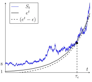
τϵ= inf{St < e−r(T−t)(ST −ϵ)} . (4.9)

On the set{τϵ< T}, the agent invests her money in the risky asset at timeτϵ. This strategy is

modeled by,

Nt=X0 er τϵ

Sτϵ

1{t≥τϵ}.

On {τϵ < T}, XT = erTX0_SS_TT−ϵ and on its complement XT =erTX0. As P(τϵ < T) >0, we

conclude that XT ≥erTX0 almost surely andP(XT > erTX0)>0.

Corollary 4.8. Let G=BT, then we have (A)H(G), (F LV R)H+(G) and (F LV R)H(G).

4.2

Example of (A)

with

v

(

H

)

<

∞

and

v

(

H

) =

∞

for

γ

∈

(0

,

1]

Here we analyze another enlargement of filtration example. It was introduced by [1] to study the case when the insider trader knows a lower or an upper bound of the stock price in a certain future horizon time. We use the initial enlargement G=F⋁σ(G) with

G=1{b1≤ST ≤b2}. (4.10)

Remark 4.9. Using the solution of the process S at time T, under constant volatility process, this problem is equivalent to,

G=1 { c1 ≤BT ≤c2 } , ci =ξlog(bi/S0) +ξ ∫ T 0 ( ξ2 2 −ηt ) dt .

As usual in this kind of problems, we have to compute the semi-martingale decomposition of process S = (St,0≤ t≤T) in the filtration G. Before that, we are going to enunciate the

results on arbitrage for the strategy setsH(G) and H+(G).

Proposition 4.10. Let G as in (4.10), then (A)H+₍

G) holds.

Proof. The result follows by the same argument of Proposition 4.7.

The Figure 1 shows an example of the situation that is described in the proof. When the stopping time happens, the insider trader invests in the stock as she knows almost surely that she will realize a positive profit.

4 EXAMPLES 14 τϵ 1 8 t St et (et−ϵ)

Figure 1: An example of realization of the stopping time τϵ defined in (4.9).

Corollary 4.11. Let G as in (4.10), then we have (A)H(G), (F LV R)H+(G) and (F LV R)H(G).

Proposition 4.12. Let G as in (4.10), then vG_{(H) = +∞.}

Proof. Consider the following stopping timeτϵ,

τϵ= inf{St < e−r(T−t)(b1−ϵ)}. (4.11)

and the strategy Θ ={(Mt, Nt) : 0≤t≤T} withNt=M X0e

r τϵ

Sτϵ 1{t≥τϵ},for some constant

M >0. On {τϵ < T},XT =erTX0 M_SS_TT−ϵ and on its complement XT =e rT_X 0, hence, E[X_TΘ] =erTX0+erTX0P(τϵ < T) [ M ST ST −ϵ −1 ] ,

which is not bounded asM → ∞ for a fixedϵ >0.

In the following, we show that the additional information carried by the filtrationGimplies

a finite terminal logarithmic utility, and therefore different for the case analyzed in Section 4.1. We assume that the processξ is constant and we start by computing the explicit expression of the drift αG = (αG_t,0 ≤t≤T) appearing in theG-semi-martingale decomposition given in

Proposition 2.9. The proof is deferred to the appendix.

Proposition 4.13. Let G as in (4.10), then

αg_t = √ ξt T −t Φ′(c_√1−Bt T−t ) −Φ′(c_√2−Bt T−t ) P(G=g|Bt) ,

and more explicitly

αg_t = ⎧ ⎪ ⎪ ⎪ ⎪ ⎪ ⎪ ⎪ ⎨ ⎪ ⎪ ⎪ ⎪ ⎪ ⎪ ⎪ ⎩ ξt √ T−t Φ′ ( c_√1−Bt T−t ) −Φ′ ( c_√2−Bt T−t ) Φ(−c_√2−Bt T−t ) + Φ(c_√1−Bt T−t ) when g= 0 , ξt √ T−t Φ′(c_√1−Bt T−t ) −Φ′(c_√2−Bt T−t ) Φ(c_√2−Bt T−t ) −Φ(c_√1−Bt T−t ) when g= 1 . (4.12)

4 EXAMPLES 15

Before the main result of this section we need to introduce the following technical lemma whose proof is deferred to the appendix.

Lemma 4.14. The integral of the functionI(x, t) defined as

I(x, t) = √ 1

T −t

[Φ′(z1)−Φ′(z2)]2

[Φ (z2)−Φ (z1)] [Φ (−z2) + Φ (z1)]

, (4.13) in the variable x∈_R is uniformly bounded for t∈[0, T]. In (4.13), we have used the following definitions z2 = (c2−x)/

√

T −t and z1 = (c1−x)/

√

T −t.

The following result shows that the logarithmic utility optimization allows for a finite opti-mum. This result was first conjectured in [1], where they supported the conjecture via numerical results. Then the conjecture was solved in the general entropy setting by [9]. Here we give a more direct proof on the line of the arguments given in [1].

Theorem 4.15. Let G as in (4.10), then uG_(H+_)<∞.

Proof. By using the expression ofαG, given in [1, Equation (4.25)], we have

E[(αG_t )2] = ξ 2 t 2π√T−t√2πt ∫ R I(x, t)e−x2/2dx

where I(x, t) is defined in (4.13) and the volatility process is bounded. By (4.4a), it is enough to prove that, for some constantK >0,

E[(αG_t)2]≤ _√ K

t(T−t) . This follows by lemma 4.14.

Proposition 4.16. Let G as in (4.10), then vG

γ(H+) = +∞ for γ ∈(1/2,1].

Proof. By Corollary 4.11 the (F LV R)H(G) condition holds and therefore an ELMM can not

exist. This implies that the Novikov condition, given in (2.6), is not satisfied. We conclude that

E[exp(1₂∫T 0 (α

G₎2_dt)]_{= +∞.Moreover, ifγ ≥1/2, it follows that γ/(1−γ)≥1 and we can}

conclude, vγ(H+) = X₀γ γ exp(γrT)E [ exp ( 1 2 γ 1−γ ∫ T 0 ( ηt−r ξt +αG_t )2 dt )] +γ 2₋₁ γ ≥ X γ 0 γ exp(γrT)E [ exp ( 1 2 ∫ T 0 ( ηt−r ξt +αG_t )2 dt )] +γ 2₋₁ γ = +∞ .

4.3

Example of (NFLVR)

with

v

(

H

)

<

∞

for

γ

∈

[0

,

1)

and

v

(

H

) = +

∞

In this section we show that the acquisition of additional information by an insider agent does not directly implies that she can take advantage of an arbitrage. Indeed we show that even knowing information about the terminal price of the risky asset (we model this by a function of BT) may not lead to an arbitrage condition.

4 EXAMPLES 16

We use the initial enlargement G=F⋁σ(G) with G=1

{

BT ∈ ∪+_k=∞−∞[2k−1,2k] }

(4.14) implying that the insider trader only knows if the Brownian motion will end up in a particular infinite union of intervals of size one. Following the same arguments of Proposition 4.13, next result gives a closed form expression of the new drift of theG-semi-martingale decomposition.

Proposition 4.17. Let G be as in (4.14), then

αg_t = √ 1 T−tP(G=g|Bt) ( _+∞ ∑ k=−∞ Φ′ ( 2_√k−Bt T −t ) −Φ′ ( 2k_√−1−Bt T−t ))

and more explicitly

αg_t = ⎧ ⎪ ⎪ ⎪ ⎪ ⎪ ⎪ ⎪ ⎨ ⎪ ⎪ ⎪ ⎪ ⎪ ⎪ ⎪ ⎩ 1 √ T −t ∑+∞ k=−∞Φ′ ( 2_√k−Bt T−t ) −Φ′(2k_√−1−Bt T−t ) ∑+∞ k=−∞Φ ( −2_√k−Bt T−t ) + Φ(2k_√−1−Bt T−t ) when g= 0 , 1 √ T −t ∑+∞ k=−∞Φ′ ( 2k_√−1−Bt T−t ) −Φ′ ( 2_√k−Bt T−t ) ∑+∞ k=−∞Φ ( 2_√k−Bt T−t ) −Φ ( 2k_√−1−Bt T−t ) when g= 1 . (4.15)

Before stating the main result of this section we state the following version of the Mean Value Theorem for definite integrals, whose proof may be found in [25, Lemma 2.1].

Lemma 4.18. Let c1 < c2, and f(·) a differentiable function. There exists ξ ∈ (c1, c2) such

that 1 c2−c1 ∫ c2 c1 f(y)dy= f(c1) +f(c2) 2 − 1 c2−c1 ∫ c2 c1 ( y−c1+c2 2 ) f′(y)dy = f(c1) +f(c2) 2 − ( ξ−c1+c2 2 ) f′(ξ) . (4.16) The following result shows that under the enlargement by the random variable in (4.14) the insider does not get any possibility of arbitrage.

Theorem 4.19. Let G be as in (4.14), then (NFLVR)_G holds.

Proof. By Corollary 2.12, it is enough to prove that the process αG satisfies the Novikov con-dition (2.6).

Using the Jensen inequality we get

E [ exp ( 1 2 ∫ T 0 (αG_t )2dt )] ≤ 1 T ∫ T 0 E [ exp [ T 2(α G t )2 ]] dt ,

so we are left to find a bound for the right hand side of the expression above. The expectation can be computed as E [ exp ( T 2(α G t )2 )] = ∑ g∈{0,1} ∫ R exp ( T 2(α g t)2 ) P(G=g|Bt=x)dP(Bt≤x) . (4.17)

Using the similarity of the the integrals for g ∈ {0,1}, we focus on getting a uniform bound integrable with respect tot in the case g= 1.

4 EXAMPLES 17

LetA=∪+_k=∞_−∞[2k−1,2k] be the set appearing in (4.14). Ifx∈A, thenP(G= 1|Bt=x)

is far from zero and the numerator of α1_t is uniformly convergent in t∈[0, T] and bounded by 2. Bounding the term P(G= 1|Bt=x) by 1 we get the following inequality

E [ exp ( T 2(α 1 t)2 )] ≤K+ ∫ Ac exp ( T 2(α 1 t)2 ) dP(Bt≤x) ,

whereK >0 is some constant.

For the moment we focus on the value of the integral in a single interval, say [c1, c2], to later

generalize the argument to the whole setAc.

In the following we assume thatx̸∈[c1, c2] and we define Φ the distribution of the standard

Gaussian andzi= (ci−x)/ √

T −twithi∈ {1,2}. By lemma 4.18, there existsζ ∈[c1, c2] such

that P(BT ∈[c1, c2]|Bt=x) = ∫ z2 z1 Φ′(u)du =√c2−c1 T−t Φ′(z1) + Φ′(z2) 2 + ( c2−c1 √ T−t− c1+c2−2x 2√T −t ) c2−c1 √ T −texp ( −(ζ−x) 2 2(T −t) ) . (4.18) Using the expression above to find an alternative form of the following term,

1 √ T−t Φ′(z1)−Φ′(z2) P(BT ∈[c1, c2]|Bt=x) = (Φ ′_(z 1)−Φ′(z2))/(Φ′(z1) + Φ′(z2)) (c2−c1)/2 + ( ζ−c1+c2 2 )_c√2−c1 T−t exp ( −(₂₍ζ−_T−x)2_t)) Φ′_(z 1)+Φ′(z2) (4.19)

that allows to show that it is bounded for all t ∈ [0, T]. It is enough to look at the limit as

t→T. The numerator is easily shown to be bounded as 0≤ lim t→T Φ′(z1)−Φ′(z2) Φ′_(z 1) + Φ′(z2) ≤ lim t→T Φ′(z1) Φ′_(z 1) + Φ′(z2) ≤1.

Therefore the boundedness follows from the fact that the denominator is sum of a constant term and another one that goes to zero. Indeed, assuming w.l.o.g. thatx < c1 < c2 – the other

case being equivalent by the symmetry of the function Φ′ –, we have

lim t→T c2−c1 √ T−texp ( −₂₍(ξ−_T−x)_t2₎) Φ′_(z 1) + Φ′(z2) = lim t→T √ 2π c2−c1 √ T−texp ( −₂₍(ξ_T−x₋)_t2₎) exp ( −(c1−x)2 2(T−t) ) + exp ( −(c2−x)2 2(T−t) ) = lim t→T √ 2π c2−c1 √ T−texp ( −(ξ−x)2−(c1−x)2 2(T−t) ) 1 + exp(−(c2−x)2−(c1−x)2 2(T−t) ) = 0.

Fixingt sufficiently near toT, we have shown that Φ′(z1)−Φ′(z2)

P (BT ∈[c1, c2]|Bt=x)

≤1 + 2

c2−c1

, x̸∈[c1, c2].

Replacing the interval [c1, c2] by the setA=∪k+=∞−∞[2k−1,2k], and by repeating the same

argument above, we get that

α1_t = ∑+∞ k=−∞Φ′ ( 2k_√−1−x T−t ) −Φ′(√2k−x T−t ) P(BT ∈A|Bt=x) ≤3, x∈Ac.

5 CONCLUSIONS 18 Finally, E [ exp ( T 2(α 1 t)2 )] ≤K+ ∫ Ac exp ( 9 2T ) dP(Bt≤x)<+∞

and the result follows.

Proposition 4.20. Let G be as in (4.14), then vG

γ(H+) < +∞ for 0 ≤ γ < 1 and vG(H) =

vG_(H+_{) = +∞.}

Proof. Similarly to the arguments used in Proposition 4.20, we can show the result starting from equations (4.4).

5

Conclusions

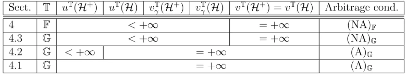
Table 1: Summary of the utility maximization problems analyzed in Section 4. Sect. _T uT_(H+_{) u}T_{(H) v}T γ(H+) vγT(H) vT(H+) = vT(H) Arbitrage cond. 4 _F <+∞ = +∞ (NA)_F 4.3 _G <+∞ = +∞ (NA)_G 4.2 _G <+∞ = +∞ (A)_G 4.1 _G = +∞ (A)_G

In this project we have analyzed the relations between the arbitrage conditions, the utility maximization problems and the enlargements of filtration. In particular we considered all these concepts with the respect to the class of strategies the agent may employ in maintaining her portfolio, by focusing on the general admissible class, H, and the one that does not allow for temporary-bankruptcy, H+_.

In terms of arbitrage, by lemma 3.4, there is practically no difference between working with the classHand the classH+_{. However in terms of utility maximization, the difference becomes}

clear as we found cases in which the (logarithmic) utility maximization is finite even in presence of arbitrage. We have included examples of this type and Table 1 shows a brief summary of the results obtained. In Section 4 we analyzed three different types of initial enlargement applied to the simple model of Geometric Brownian motion. Finally a very interesting result has been given in Section 4.3, showing that an enlargement of initial type does not immediately implies that the insider plays in a condition of arbitrage.

Acknowledgments

This research was partially supported by the Spanish Ministry of Economy and Competitiveness grants MTM2017-85618-P (via FEDER funds) and MTM2015–72907–EXP.

Conflict of interest

REFERENCES 19

References

[1] I. Pikovsky and I. Karatzas. Anticipative portfolio optimization. Advances in Applied Probability, 28(4):1095–1122, 1996.

[2] R. C. Merton. Lifetime portfolio selection under uncertainty: The continuous-time case. The Review of Economics and Statistics, 51(3):247–257, 1969.

[3] R. C. Merton. Optimum consumption and portfolio rules in a continuous-time model. Journal of economic theory, 3(4):373–413, 1971.

[4] T. Jeulin and M. Yor. Nouveaux r´esultats sur le grossissement des tribus. Annales scien-tifiques de l’ ´Ecole Normale Sup´erieure, 4e s´erie, 11(3):429–443, 1978.

[5] J. Jacod. Grossissement initial, hypoth´ese (h’) et th´eor´eme de girsanov. InGrossissements de filtrations: exemples et applications, pages 15–35. Springer, 1985.

[6] M. Chaleyat-Maurel and T. Jeulin. Grossissement gaussien de la filtration brownienne. In Thomas Jeulin and Marc Yor, editors, Grossissements de filtrations: exemples et applica-tions, pages 59–109, Berlin, Heidelberg, 1985. Springer Berlin Heidelberg.

[7] H. F¨ollmer and P. Imkeller. Anticipation cancelled by a girsanov transformation: a paradox on wiener space. Annales de l’IHP Probabilit´es et statistiques, 29(4):569–586, 1993. [8] A. Grorud and M. Pontier. Insider trading in a continuous time market model.International

Journal of Theoretical and Applied Finance, 01(03):331–347, 1998.

[9] J. Amendinger, P. Imkeller, and M. Schweizer. Additional logarithmic utility of an insider. Stochastic Processes and their Applications, 75(2):263–286, 1998.

[10] J. Amendinger, D. Becherer, and M. Schweizer. A monetary value for initial information in portfolio optimization. Finance and Stochastics, 7(1):29–46, 2003.

[11] S. Dereich S. Ankirchner and P. Imkeller. The shannon information of filtrations and the additional logarithmic utility of insiders. The Annals of Probability, 34(2):743–778, 2006. [12] F. Baudoin and L. Nguyen-Ngoc. The financial value of a weak information on a financial

market. Finance and Stochastics, 8(3):415–435, August 2004.

[13] F. Biagini and B. Øksendal. A general stochastic calculus approach to insider trading. Applied Mathematics and Optimization, 52(2):167–181, July 2005.

[14] B. D’Auria, D. Garc´ıa, and J. A. Salmer´on. Optimal portfolio with insider information on the stochastic interest rate, 2017.

[15] A. Aksamit and M. Jeanblanc. Enlargement of Filtration with Finance in View. Springer International Publishing, 2017.

[16] S. Ankirchner and P. Imkeller. Finite utility on financial markets with asymmetric informa-tion and structure properties of the price dynamics. Annales de l’Institut Henri Poincar´e, Statistics, 41(3):479––503, 2005.

[17] B. Acciaio, C. Fontana, and C. Kardaras. Arbitrage of the first kind and filtration enlarge-ments in semimartingale financial models. Stochastic Processes and their Applications, 126(6):1761–1784, 2016.

REFERENCES 20

[18] H. N. Chau, A. Cosso, and C. Fontana. The value of informational arbitrage. arXiv preprint, 2018.

[19] H. N. Chau, W. Runggaldier, and P. Tankov. Arbitrage and utility maximization in market models with an insider. Mathematics and Financial Economics, 12(4):589–614, 2018. [20] F. Delbaen. Representing martingale measures when asset prices are continuous and

bounded. Mathematical Finance, 2(2):107–130, 1992.

[21] F. Delbaen and W. Schachermayer. A general version of the fundamental theorem of asset pricing. Mathematische annalen, 300(1):463–520, 1994.

[22] F. Delbaen and W. Schachermayer. The Mathematics of Arbitrage. Springer Finance. Springer-Verlag, 2006.

[23] F. Baudoin. Conditioned stochastic differential equations: theory, examples and application to finance. Stochastic Processes and their Applications, 100(1):109–145, 2002.

[24] N. Bauerle and U. Rieder. Portfolio optimization with markov-modulated stock prices and interest rates. IEEE Transactions on Automatic Control, 15(3):442–447, 2004.

[25] S. Dragomir and R. Agarwa. Two inequalities for differentiable mappings and applications to special means of real numbers and to trapezoidal formula. Applied Mathematical Letters, 11(5):91––95, 1997.

Appendix

Proof of Proposition 4.13. The following proof is along the line the one used in [14, Proposition 14] in the context of the Ornstein-Uhlenbeck process.

Applying the definition of conditional expectation and considering the random variable

G=1{c1≤BT ≤c2} E[1{c1 ≤BT ≤c2}αG] =E [ 1{c1 ≤BT ≤c2}αBT ] ,

and from this fact we deduce that the processαG _{takes the following form,}

α1_t = ∫c2 c1 α BT_dΦ ( B_√T−Bt T−t ) P(BT ∈(c1, c2)|Bt) (5.1a) α0_t = ∫c1 −∞αBT dΦ ( B_√T−Bt T−t ) +∫_c+∞ 2 α BT_dΦ ( B_√T−Bt T−t ) P(BT ̸∈(c1, c2)|Bt) , (5.1b) where Φ(·) is the distribution of the standard Gaussian random variable. Substituting in (5.1a) the explicit expression of αBT_{, given in (4.6), the numerator can be written in the following}

form ∫ c2 c1 αBT_dΦ ( B_√T −Bt T−t ) = ∫ c2 c1 BT −Bt T−t dΦ ( B_√T −Bt T−t ) =E [ (1{BT ≥c2}+1{BT ≤c1}) BT −Bt T−t |Bt ] = √ 1 T−t ( Φ′ ( c2−Bt √ T−t ) −Φ′ ( c1−Bt √ T −t )) ,

REFERENCES 21

where we have used again that E[1{Z ≥c}(Z−µ)] =σ2fZ(c) ifZ ∼dN(µ, σ2). Substituting

back in (5.1a) we finally get,

α1_t = √ 1 T −t Φ′ ( c_√2−Bt T−t ) −Φ′ ( c_√1−Bt T−t ) P(BT ∈(c1, c2)|Bt) , (5.2)

and we get the result.

Proof of lemma 4.14. We start by splitting R in three intervals (−∞, c1], (c1, c2) and [c2,∞),

then we prove that on each interval the integral is finite.

Interval (−∞, c1]: We apply a change of variable in z1 and express z2 = z1 + (c2 − c1)/

√

T −t. We let st:= (c2−c1)/

√

T−tand call its minimum in tas s0 >0. We get ∫ c1 −∞ I(x, t)dx= ∫ +∞ 0 [Φ′(z1)−Φ′(z1+st)]2 [Φ (z1+st)−Φ (z1)] [Φ (−z1−st) + Φ (z1)] dz1 = ∫ +∞ 0 ( [Φ′(z1)−Φ′(z1+st)]2 Φ (z1+st)−Φ (z1) +[Φ ′_(z 1)−Φ′(z1+st)]2 Φ (−z1−st) + Φ (z1) ) dz1 . (5.3)

We continue by showing that both terms are finite. We first consider the first term.

∫ +∞ 0 [Φ′(z1)−Φ′(z1+st)]2 Φ (z1+st)−Φ(z1) dz1 ≤ ∫ +∞ 0 [Φ′(z1)−Φ′(z1+st)]2 Φ (z1+s0)−Φ(z1) dz1 ≤ ∫ +∞ 0 [Φ′(z1)]2 Φ (z1+s0)−Φ(z1) dz1 .

The integral in [0,1] is clearly bounded. While for the interval [1,+∞], we apply a comparison criteria with the functionf(z) = 1/z2, as follows,

lim z1→∞ z₁2 [Φ ′_(z 1)]2 Φ (z1+s0)−Φ(z1) = lim z1→∞ 1 √ 2π z₁2[exp(−z₁2/2)]2 ∫z1+s0 z1 exp(−u 2_/2)du = lim z1→∞ 1 √ 2π 2z1 [ exp(−z₁2/2)]2−2z₁3[exp(−z₁2/2)]2 exp(−(z1+s0)2/2)−exp(−z12/2) = lim z1→∞ 1 √ 2π 2z1exp ( −z2₁/2) −2z₁3exp( −z₁2/2) exp(−z1s0) exp(−s2₀/2)−1 →0 .

In the second equality above, we used L’Hopital Rule and we conclude that the integral is finite on (1,+∞).

As for the second term in (5.3), we have the following bound,

∫ +∞ 0 [Φ′(z1)−Φ′(z1+st)]2 Φ(−z1−st) + Φ(z1) dz1 ≤ ∫ +∞ 0 [Φ′(z1)−Φ′(z1+st)]2 Φ(z1) dz1 ≤2 ∫ +∞ 0 [ Φ′(z1)−Φ′(z1+st) ]2 dz1 ≤2 ∫ +∞ 0 [ Φ′(z1) ]2 dz1= 1 √ 2 .

Interval[c2,+∞): We proceed in the same way as above, now applying a change of variable

inz2. ∫ +∞ c2 I(x, t)dx= ∫ 0 −∞ [Φ′(z2−st)−Φ′(z2)]2 [Φ (z2)−Φ (z2−st)] [Φ (−z2) + Φ (z2−st)] dz2 = ∫ 0 −∞ ( [Φ′(z2−st)−Φ′(z2)]2 Φ (z2)−Φ (z2−st) +[Φ ′_(z 2−st)−Φ′(z2)]2 Φ (−z2) + Φ (z2−st) ) dz2 (5.4)

REFERENCES 22

We show that both terms in (5.4) are finite. For the first one we have

∫ 0 −∞ [Φ′(z2−st)−Φ′(z2)]2 Φ (z2)−Φ (z2−st) dz2 ≤ ∫ 0 −∞ [Φ′(z2−st)−Φ′(z2)]2 Φ (z2)−Φ (z2−s0) dz2≤ ∫ 0 −∞ [Φ′(z2)]2 Φ (z2)−Φ (z2−s0) dz2 ,

and applying the same reasoning as before, we conclude that the integral is finite. Then for the second term we have

∫ 0 −∞ [Φ′(z2−st)−Φ′(z2)]2 Φ (−z2) + Φ (z2−st) dz2 ≤ ∫ 0 −∞ [Φ′(z2−st)−Φ′(z2)]2 Φ (−z2) dz2 ≤2 ∫ 0 −∞ [ Φ′(z2) ]2 dz2 = 1 √ 2 .

Interval (c1, c2): We proceed by applying a change of variable, and we arbitrarily choose

to do it in the variable z2. We get ∫ c2 c1 I(x, t)dx= ∫ st 0 [ [Φ′(z2)−Φ′(z2−st)]2 Φ(z2)−Φ(z2−st) +[Φ ′_(z 2)−Φ′(z2−st)]2 Φ(−z2) + Φ(z2−st) ] dz2 (5.5)

and again we show that both integrals in (5.5) are bounded. For the first integral we have

∫ st 0 [Φ′(z2)−Φ′(z2−st)]2 Φ(z2)−Φ(z2−st) dz2= 2 ∫ st/2 0 [Φ′(z2)−Φ′(z2−st)]2 Φ(z2)−Φ(z2−st) dz2≤2 ∫ st/2 0 [Φ′(z2)]2 Φ(z2)−Φ(z2−s0) dz2 ≤2 ∫ ∞ 0 [Φ′(z2)]2 Φ(z2)−Φ(z2−s0) dz2

where the first equality holds because the function we are integrating is symmetric with respect

st/2. The last integral is finite as it is trivially so on [0,1] and using a comparison criteria with

the functionf(z) = 1/z2it is also integrable on [1,+∞]. In a similar way we analyze the second integral in (5.5) and by symmetry of the function with respect to thest/2 we get

∫ st 0 [Φ′(z2)−Φ′(z2−st)]2 Φ(−z2) + Φ(z2−st) dz2= 2 ∫ st/2 0 [Φ′(z2)−Φ′(z2−st)]2 Φ(−z2) + Φ(z2−st) dz2 .

Then we compute the following bound Φ′(z2)−Φ′(z2−st) = 1 √ 2π [ exp ( −z 2 2 2 ) −exp ( −(z2−st) 2 2 )] =√1 2πexp ( −z 2 2 2 ) [ 1−exp ( −s 2 t −2z2st 2 )] ≤√1 2πexp ( −z 2 2 2 ) ,

where the last inequality holds because s2

t −2z2st≥0 as 0≤z2≤st/2. ∫ st 0 [Φ′(z2)−Φ′(z2−st)]2 Φ(−z2) + Φ(z2−st) dz2≤ √ 2 π ∫ st/2 0 exp(−z₂2) Φ(−z2) + Φ(z2−st) dz2 ≤ ∫ st/2 0 exp(−z2₂) Φ(−z2) dz2 ≤ ∫ 1 0 exp( −z₂2) Φ(−z2) dz2+ ∫ +∞ 1 exp( −z₂2) Φ(−z2) dz2 .

The first integral is trivially bounded. For the second to be bounded, we apply a comparison criteria with the function f(z) = 1/z2. Putting together the given bounds we may bound the integral in (5.5) and the proof is finished.

Proof of Proposition 4.17. Applying the definition of conditional expectation and considering the random variable G=1

{ BT ∈ ∪+_k=∞−∞[2k−1,2k] } , E[1 { BT ∈ ∪+_k=∞−∞[2k−1,2k] } αG] =E [ 1{BT ∈ ∪+_k=∞−∞[2k−1,2k] } αBT ] ,

REFERENCES 23

and from this fact we deduce that the processαG takes the following form,

α1_t = √ 1 T−t ∑+∞ k=−∞ ∫2k 2k−1αBTdΦ ( B_√T−Bt T−t ) P(G= 1|Bt) (5.6a) α0_t = √ 1 T−t ∑+∞ k=−∞ ∫2k+1 2k αBTdΦ ( B_√T−Bt T−t ) P(G= 0|Bt) , (5.6b) where Φ(·) is the distribution of the standard Gaussian random variable. We can deal each sum of the numerator as we did in equations (5.1a)-(5.1b) and we get the result.