Archive University of Zurich Main Library Strickhofstrasse 39 CH-8057 Zurich www.zora.uzh.ch Year: 2015
Approximate bayesian model selection with the deviance statistic Held, Leonhard ; Sabanés Bové, Daniel ; Gravestock, Isaac
Abstract: Bayesian model selection poses two main challenges: the specification of parameter priors for all models, and the computation of the resulting Bayes factors between models. There is now a large literature on automatic and objective parameter priors in the linear model. One important class are g-priors, which were recently extended from linear to generalized linear models (GLMs). We show that the resulting Bayes factors can be approximated by test-based Bayes factors (Johnson [ Scand. J. Stat. 35 (2008) 354–368]) using the deviance statistics of the models. To estimate the hyperparameter g, we propose empirical and fully Bayes approaches and link the former to minimum Bayes factors and shrinkage estimates from the literature. Furthermore, we describe how to approximate the corresponding posterior distribution of the regression coefficients based on the standard GLM output. We illustrate the approach with the development of a clinical prediction model for 30-day survival in the GUSTO-I trial using logistic regression.
DOI: https://doi.org/10.1214/14-STS510
Posted at the Zurich Open Repository and Archive, University of Zurich ZORA URL: https://doi.org/10.5167/uzh-117659
Journal Article Published Version Originally published at:
Held, Leonhard; Sabanés Bové, Daniel; Gravestock, Isaac (2015). Approximate bayesian model selection with the deviance statistic. Statistical science, 30(2):242-257.
DOI:10.1214/14-STS510
©Institute of Mathematical Statistics, 2015
Approximate Bayesian Model Selection
with the Deviance Statistic
Leonhard Held, Daniel Sabanés Bové and Isaac Gravestock
Abstract. Bayesian model selection poses two main challenges: the spec-ification of parameter priors for all models, and the computation of the re-sulting Bayes factors between models. There is now a large literature on au-tomatic and objective parameter priors in the linear model. One important class are g-priors, which were recently extended from linear to generalized linear models (GLMs). We show that the resulting Bayes factors can be ap-proximated by test-based Bayes factors (Johnson [Scand. J. Stat.35 (2008) 354–368]) using the deviance statistics of the models. To estimate the hyper-parameterg, we propose empirical and fully Bayes approaches and link the former to minimum Bayes factors and shrinkage estimates from the litera-ture. Furthermore, we describe how to approximate the corresponding pos-terior distribution of the regression coefficients based on the standard GLM output. We illustrate the approach with the development of a clinical predic-tion model for 30-day survival in the GUSTO-I trial using logistic regression.
Key words and phrases: Bayes factor, deviance, generalized linear model, g-prior, model selection, shrinkage.
1. INTRODUCTION
The problem of model and variable selection is per-vasive in statistical practice. For example, it is cen-tral for the development of clinical prediction models [Steyerberg (2009)]. For illustration, we consider the GUSTO-I trial, a large randomized study for compar-ison of four different treatments in over 40,000 acute myocardial infarction patients [Lee et al.(1995)]. We study a publicly available subgroup from the Western region of the USA withn=2188 patients and progno-sis of the binary endpoint 30-day survival [Steyerberg (2009)]. In order to develop a clinical prediction model for this endpoint, we focus our analysis on the assess-ment of the effects of 17 covariates listed in Table1in a logistic regression model.
Leonhard Held is Professor and Isaac Gravestock is Ph.D. Student, Department of Biostatistics, Institute of
Epidemiology, Biostatistics and Prevention, University of Zurich, Hirschengraben 84, 8001 Zurich, Switzerland (e-mail:[email protected];[email protected]). Daniel Sabanés Bové is Biostatistician at F. Hoffmann-La Roche Ltd, 4070 Basel, Switzerland (e-mail:
There is now a large literature on automatic and ob-jective Bayesian model selection, which unburden the statistician from eliciting manually the parameter pri-ors for all models in the absence of substantive prior information [see, e.g., Berger and Pericchi (2001)]. However, such objective Bayesian methodology is cur-rently limited to the linear model [e.g., Bayarri et al. (2012)], where the g-prior on the regression coeffi-cients is the standard choice [Liang et al. (2008)]. For non-Gaussian regression, there are computational and conceptual problems, and one solution to this are test-based Bayes factors [Johnson(2005)]. Consider a classical scenario with a null model nested within a more general alternative model. Traditionally, the use of Bayes factors requires the specification of proper prior distributions on all unknown model parameters of the alternative model, which are not shared by the null model. In contrast,Johnson(2005) defines Bayes factors using the distribution of a suitable test statistic under the null and alternative models, effectively re-placing the data with the test statistic. This approach eliminates the necessity to define prior distributions on model parameters and leads to simple closed-form ex-pressions forχ2-,F-,t-, andz-statistics.
TABLE1
Description of the variables in the GUSTO-I data set
Variable Description
y Death within 30 days after acute myocardial infarction (Yes=1, No=0) x1 Gender (Female=1, Male=0)
x2 Age [years]
x3 Killip class (4 categories)
x4 Diabetes (Yes=1, No=0)
x5 Hypotension (Yes=1, No=0)
x6 Tachycardia (Yes=1, No=0)
x7 Anterior infarct location (Yes=1, No=0)
x8 Previous myocardial infarction (Yes=1, No=0)
x9 Height [cm]
x10 Weight [kg]
x11 Hypertension history (Yes=1, No=0)
x12 Smoking (3 categories: Never/Ex/Current)
x13 Hypercholesterolaemia (Yes=1, No=0)
x14 Previous angina pectoris (Yes=1, No=0)
x15 Family history of myocardial infarctions (Yes=1, No=0) x16 ST elevation on ECG: Number of leads (0–11)
x17 Time to relief of chest pain more than 1 hour (Yes=1, No=0)
TheJohnson(2005) approach is extended inJohnson (2008) to the likelihood ratio test statistic and, thus, if applied to generalized linear regression models (GLMs), to the deviance statistic [Nelder and Wed-derburn (1972)]. This is explored further in Hu and Johnson (2009), where Markov chain Monte Carlo (MCMC) is used to develop a Bayesian variable se-lection algorithm for logistic regression. However, the factorg in the implicit g-prior is treated as fixed and estimation of the regression coefficients is also not dis-cussed. We fill this gap and extend the work by Hu and Johnson (2009), combining g-prior methodology for the linear model with Bayesian model selection based on the deviance. This enables us to apply em-pirical [George and Foster(2000)] and fully Bayesian [Cui and George (2008)] approaches for estimating the hyperparametergto GLMs. By linkingg-priors to the theory on shrinkage estimates of regression coeffi-cients [Copas(1983, 1997)], we finally obtain a unified framework for objective Bayesian model selection and parameter inference for GLMs.
The paper is structured as follows. In Section2 we review theg-prior in the linear and generalized linear model, and show that this prior choice is implicit in the application of test-based Bayes factors computed from the deviance statistic. In Section 3 we describe how the hyperparameter g influences model selection and parameter inference, and introduce empirical and fully
Bayesian inference for it. Using empirical Bayes to es-timate g, we are able to analytically quantify the ac-curacy of test-based Bayes factors in the linear model. Connections to the literature on minimum Bayes fac-tors and shrinkage of regression coefficients are out-lined. In Section4we apply the methodology in order to build a logistic regression model for predicting 30-day survival in the GUSTO-I trial, and compare our methodology with selected alternatives in a bootstrap study. In Section 5 we summarize our findings and sketch possible extensions.
2. OBJECTIVE BAYESIAN MODEL SELECTION IN REGRESSION
Consider a generic regression modelMwith linear predictorη=α+x⊤β, from which we assume that the outcome y=(y1, . . . , yn) was generated. We collect
the intercept α, the regression coefficients vector β, and possible additional parameters (e.g., the residual variance in a linear model) in θ ∈. Specific candi-date modelsMj,j∈J, differ with respect to the con-tent and the dimension of the covariate vector x, and henceβ, so each modelMj defines its own parameter vectorθj with likelihood function p(y|θj,Mj).
Through optimizing this likelihood, we obtain the maximum likelihood estimate (MLE) θˆj of θj. For
Bayesian inference a prior distribution with density p(θj|Mj)is assigned to the parameter vectorθj to
p(y|θj,Mj)p(θj|Mj). This forms the basis to
com-pute the posterior mean E(θj|y,Mj) and other
suit-able characteristics of the posterior distribution. The marginal likelihood
p(y|Mj)=
j
p(y|θj,Mj)p(θj|Mj) dθj
is the key ingredient to transform prior model probabil-itiesPr(Mj),j ∈J, to posterior model probabilities
Pr(Mj|y)= p(y|Mj)Pr(Mj) k∈Jp(y|Mk)Pr(Mk) (1) = DBFj,0Pr(Mj) k∈JDBFk,0Pr(Mk) .
In the second line, the usual (data-based) Bayes factor DBFj,0=p(y|Mj)/p(y|M0) of model Mj versus a
reference model M0 replaces the marginal likelihood p(y|Mj) from the first line. Improper priors can only be used for parameters that are common to all models (e.g., here the interceptα), because only then the inde-terminate normalizing constant cancels in the posterior model probabilities (1).
In Section2.1we discuss theg-prior, a specific class of prior distributions p(θj|Mj), commonly used in
linear model selection problems. The g-prior induces shrinkage of β, in the sense that the posterior mean is a shrunken version of the MLE toward the prior mean. Furthermore, it is an automatic prior, since it does not require specification of subjective prior infor-mation. Section2.2 discusses the resulting test-based Bayes factors under theg-prior.
2.1 Zellner’sg-Prior and Generalizations
We start with the original formulation of Zellner’s g-prior for the Gaussian linear model in Section 2.1.1 and extend this to GLMs in Section2.1.2.
2.1.1 Gaussian linear model. Consider the Gaus-sian linear modelMj:yi∼N(α+x⊤ijβj, σ2)with in-terceptα, regression coefficients vector βj, and vari-ance σ2, and collect all parameters in θj =(α,β⊤j,
σ2)⊤. Here N(μ, σ2) denotes the univariate Gaus-sian density with mean μand variance σ2, and xij =
(xi1, . . . , xidj)⊤is the covariate vector for observation
i=1, . . . , n. Using then×dj full rank design matrix
Xj =(x1j, . . . ,xnj)⊤, the likelihood obtained from n
independent observations is p(y|θj,Mj)=Nn y|α1+Xjβj, σ2I , (2)
with 1 and I denoting the all-ones vector and iden-tity matrix of dimension n, respectively. We assume
that the covariates have been centered around 0, that is, X⊤j 1=0. Here and in the following,0 denotes the zero vector of lengthdj.
Zellner’s g-prior [Zellner (1986)] fixes a constant g >0 and specifies the Gaussian prior
βj|σ2,Mj ∼Ndj
0, gσ2X⊤j Xj
−1 (3)
for the regression coefficients βj, conditional on σ2. This prior can be interpreted as a posterior distribu-tion, if α is fixed and a locally uniform prior for βj is combined with an imaginary outcomey0=α1from the Gaussian linear model (2) with the same design ma-trixXj but scaled residual variancegσ2. The prior (3)
onβj is usually combined with an improper reference prior on the intercept α and the residual variance σ2 [Liang et al. (2008)]: p(α, σ2)∝σ−2. The posterior distribution of(α,β⊤j )⊤is then a multivariatet distri-bution, with posterior mean ofβj given by
E(βj|y,Mj)= g
g+1βˆj =
n· ˆβj +n/g·0
n+n/g . (4)
This means that the MLEβˆj, the ordinary least squares (OLS) estimate, is shrunk toward the prior mean zero. The shrinkage factort=g/(g+1)scales the MLE to obtain the posterior mean (4). In other words, the pos-terior mean is a weighted average of the MLE and the prior mean with weights proportional to the data sam-ple size n and the term n/g, respectively. Thus, n/g can be interpreted as the prior sample size, or 1/g as the relative prior sample size. The question of how to choose or estimategwill be addressed in Section3.
One advantage of Zellner’s g-prior is that the marginal likelihood, or, equivalently, the (data-based) Bayes factor versus the null model M0:βj =0, has a simple closed-form expression in terms of the usual coefficient of determination Rj2 of model Mj [Liang et al.(2008)]: DBFj,0 (5) =(g+1)(n−dj−1)/21+g1−R2 j −(n−1)/2 . Note that Rj2 can be written as a function of the F -statistic Fj =(n−dj−1)Rj2 /dj1−Rj2 (6)
for testing βj =0. This suggests that similar expres-sions (in terms of test statistics) can be derived for the corresponding Bayes factors in GLMs. This conjecture will be confirmed in Section2.2.
2.1.2 Generalized linear model. Now consider a GLMMj with linear predictorηij=α+x⊤ijβj, mean μij=h(ηij)obtained with the response functionh(η)
and variance function v(μ) [Nelder and Wedderburn (1972)]. The direct extension of the standard g-prior in the Gaussian linear model is then the generalized g-prior [Sabanés Bové and Held(2011a)]
βj|Mj ∼Ndj
0, gcX⊤j WXj−1,
(7)
whereWis a diagonal matrix with weights for the ob-servations (e.g., the binomial sample sizes for logistic regression). Here the appropriate centering of the co-variates is X⊤jW1=0. As in Section 2.1.1, we spec-ify an improper uniform prior p(α) ∝1 for the in-tercept α. The constant c =v{h(α)}h′(α)−2 [Copas (1983); Sabanés Bové and Held (2011a)] in (7) cor-responds to the varianceσ2in the standardg-prior (3), which could also be formulated for general linear mod-els with a nonunit weight matrix W. It preserves the interpretation of n/g as the prior sample size. Note thatSabanés Bové and Held(2011a) recommend to use α=0 as default, but considerable improvements in ac-curacy can be obtained by using the MLEαˆ ofαunder the null model; see Section4.1for details.
The connection between (3) and (7) is as follows. Denote the expected Fisher information (conditional on the variance σ2 in the Gaussian linear model) for (α,β⊤j)⊤ as I(α,βj). In the Gaussian linear model, this(dj +1)×(dj +1)matrix is block-diagonal due
to the centering of the covariates, and does not depend on the intercept nor the regression coefficients:
I(α,βj)= I α,α Iα,βj I⊤ α,βj Iβj,βj =σ−2 n 0⊤ 0 X⊤j Xj . Hence, (3) can be written as
βj|Mj ∼Ndj 0, g·Iβ−1 j,βj . (8)
In the GLM,I(α,βj)depends on the parameters and is not necessarily block-diagonal. However, if we fix βj at its prior mean0,I(α,βj =0)is block-diagonal withIβ
j,βj =c−
1X⊤
jWXj, so (7) and (8) are
equiva-lent; seeCopas[(1983), Section 8] for details. Depar-tures from the assumptionβj =0are also discussed in Copas(1983).
In contrast to Gaussian linear models, the marginal likelihood for GLMs no longer has a closed-form ex-pression. For its computation, one has to resort to nu-merical approximations, for example, a Laplace ap-proximation. This requires a Gaussian approximation of the posterior p(α,βj|y,Mj), which can be obtained
with the Bayesian iteratively weighted least squares al-gorithm. See Sabanés Bové and Held [(2011a), Sec-tion 3.1] for more details.
2.2 Test-Based Bayes Factors
Based on the asymptotic distribution of the deviance statistic in Section2.2.1, we connect the resulting test-based Bayes factors with the g-prior in Section 2.2.2 and discuss the advantages over data-based Bayes fac-tors in Section2.2.3.
2.2.1 Asymptotic distributions of the deviance statis-tic. Consider the frequentist approach to model selec-tion, where test statistics are used to assess the evi-dence against the null modelM0:βj =0in a specific GLMMj. A popular choice is the deviance (or likeli-hood ratio test) statistic
zj(y)=2 log maxα,β jp(y|α,βj,Mj) maxαp(y|α,M0) . Then we have the well-known result that, conditional on M0, the distribution of the deviance zj(Y)
con-verges forn→ ∞to a chi-squared distributionχ2(dj)
withdj degrees of freedom.
To derive the asymptotic distribution of the deviance statistic under model Mj, Johnson (2008) considers a sequence of local alternative hypotheses H1n:βj = O(1/√n), so the size of the true regression coefficients is scaled with 1/√n, and thus gets smaller with in-creasing number of observationsn. This is the case of practical interest, because for largerβj it would be triv-ial to differentiate betweenH0:βj =0andH1n, and for smaller βj it would be too difficult [Johnson (2005), page 691]. In this setup, the distribution of the deviance converges forn→ ∞to a noncentral chi-squared dis-tributionχ2(dj, λj)withdj degrees of freedom, where
λj =β⊤j Iβj,βjβj is the noncentrality parameter. Here
Iβ
j,βj denotes the expected Fisher information forβj
in model Mj, evaluated at βj =0. See Appendix A for a proof of this.
2.2.2 Defining the test-based Bayes factor. We now specify the generalized g-prior (8) for βj in the al-ternative modelMj withgfixed. For the noncentral-ity parameter λj =β⊤j Iβj,βjβj, this corresponds to
the gamma prior λj ∼G(dj/2,1/(2g)) (see also
Ap-pendixA). From above we have the approximate “like-lihood”zj|λj ∼a χ2(dj, λj)of the deviance statisticzj.
Johnson(2008), Theorem 2, shows that the implied ap-proximate marginal distribution ofzj is
zj a ∼Gdj/2,1/ 2(g+1), (9)
which gives the approximate “marginal likelihood” papprox(zj|Mj) of model Mj in terms of the
de-viance statisticzj. Furthermore, we have the
approxi-mate “marginal likelihood” papprox(zj|M0)of the null
model M0 from zj a
∼G(dj/2,1/2). With these
pre-requisites, we can derive the test-based Bayes factor
(TBF) [Johnson(2008)] TBFj,0= papprox(zj|Mj) papprox(zj|M0) (10) =(g+1)−dj/2exp g g+1 zj 2
of model Mj versus model M0 for fixed g. TBFj,0 approximates the data-based Bayes factor DBFj,0 = p(y|Mj)/p(y|M0) obtained with the generalized g -prior (8).
It is instructive to compare the TBF (10) with the DBF (5) in the linear model if g is fixed at the same value. Assume that 0< R2j <1. Then we have zj =
−nlog(1−R2j) and (10) can be written as TBFj,0= (g+1)−dj/2(1−R2
j)−gn/{2(g+1)}. On the other hand,
we have DBFj,0=(g+1)(n−dj−1)/2 ·(g+1)1−R2j+Rj2−(n−1)/2 < (g+1)(n−dj−1)/2(g+1)1−R2 j −(n−1)/2 =(g+1)−dj/21−R2 j −(n−1)/2 =TBFj,01−Rj2 {1−n/(g+1)}/2 ≤TBFj,0 ifg≥n−1.
Hence, in the linear model, TBFj,0 will be larger than DBFj,0if both are calculated with the sameg≥n−1; however, it is not clear which Bayes factor is larger for g < n−1. In Section3.2.2we provide a comparison of DBFs and TBFs in the case wheregis not fixed at the same value, but estimated separately via empirical Bayes.
2.2.3 Advantages of the test-based Bayes factor. Hu and Johnson (2009) emphasize that TBFs behave like ordinary Bayes factors, in the sense that for a se-quence of nested models M0⊂M1⊂M2, we have TBF2,0 =TBF2,1 ·TBF1,0. Hence, it is possible to compute coherent posterior model probabilities from (1) using TBFs in place of DBFs. These probabil-ities will be invariant to the choice of the baseline
model M0, in our case the null model. The availabil-ity of posterior model probabilities is a clear advan-tage over theP-values obtained from a classical anal-ysis of deviance, which are informal and indirect mea-sures of evidence [see, e.g., Goodman (1999a)], and only suitable for pairwise model comparisons. In addi-tion, the Bayesian approach offers other posterior prob-abilities of interest, for example, inclusion probabili-ties, which are easy to interpret and are required to compute the median probability model [Barbieri and Berger(2004)].
Furthermore, the TBF can be computed much more easily than the DBF because it only requires the de-viance statisticzj, which can by calculated by standard
GLM fitting software. No computation of the expected Fisher information Iβ
j,βj =c−
1X⊤
j WXj is required,
as it is only implicitly used in the prior formulation. In contrast, the DBF does not have a closed form and thus needs to be approximated by numerical means, which requires explicit calculation of the inverse of Iβ
j,βj.
The computational advantages of TBFs over DBFs in-crease further whengis treated as unknown; see Sec-tion3.
3. CALIBRATING THEG-PRIOR
How does the prior variance factorgin the general-izedg-prior (8) influence posterior inference? We will look at the implications on shrinkage and model selec-tion in Secselec-tion3.1, and estimategfrom the data using empirical Bayes (Section 3.2) and fully Bayes (Sec-tion3.3) procedures.
3.1 The Role ofgfor Shrinkage and Model Selection
We first look at the role of g for shrinkage in a GLM, following the arguments byCopas(1983). It is well known from standard GLM theory that the MLE
ˆ
θj =(α,ˆ βˆ⊤j )⊤follows asymptotically a normal
distri-bution with meanθj and covariance matrix equal to the
inverse expected Fisher informationI(α,βj)−1, eval-uated at the true valuesαandβj. As inCopas(1983), we replace βj with its prior mean 0, that is, we as-sume that the asymptotic inverse covariance matrix of
ˆ
θj isI(α,0)=diag{Iα,α,Iβj,βj}. Note thatαˆ andβˆj
are now uncorrelated because we have centered the co-variate vectors such thatX⊤j W1=0.
Combining this Gaussian “likelihood” ofθj with the
generalizedg-prior θj|g,Mj ∼Ndj+1 0 0 , ∞ 0 0 g·Iβ−1 j,βj
gives the posterior distribution θj|y, g,Mj (11) ∼Ndj+1 ˆ α t· ˆβj , I−1 α,α 0 0 t·Iβ−1 j,βj . Here t =g/(g+1) is the same shrinkage factor for
ˆ
βj as in the Gaussian linear model from Section2.1.1.
A smallerg leads to a smaller t and thus to stronger shrinkage of theβj posterior toward 0. The approxi-mate posterior covariance matrix ofβj is also shrunk by the shrinkage factort compared to the frequentist covariance matrix. In Section4.2we provide an empir-ical comparison of the true shrinkage under the gener-alizedg-prior and the theoretical shrinkageg/(g+1). The above assumption that the covariance matrix of the MLE is the inverse expected Fisher information I(α,0)−1 enables us to derive a simple form of the posterior distribution. In practice, we use the corre-sponding sub-matrices of the observed Fisher informa-tion matrix evaluated at the MLE, easily available from fitting a standard GLM, and (11) holds only approxi-mately. Likewise, the interpretion ofgas the ratio be-tween the data sample size and the prior sample size holds only approximately.
In order to understand the role ofgfor model selec-tion, consider the TBF formula (10) and the limiting case ofg→0. Then the generalizedg-prior converges to a point mass atβj =0, and thus Mj collapses to the null model M0. Consequently, TBFj,0 →1, be-cause both models are equal descriptions of the data in the limit. On the other extreme, the caseg→ ∞ cor-responds to an increasingly vague prior on βj. As is well known, arbitrarily inflating the prior variance of parameters that are not common to all models is not a safe strategy. Here we see immediately from (10) that TBFj,0 →0 in this case. This means that no matter how well the modelMj fits the data compared to the null modelM0, the latter is preferred if g is chosen large enough. This is an example of Lindley’s paradox [Lindley(1957)].
In between these two extremes, quite a few fixed values forg have been recommended. The choice of g=ncorresponds to the unit information prior [Kass and Wasserman(1995)], where the relative prior sam-ple size is 1/n. For large n, the TBF is asymptoti-cally (n→ ∞) equivalent to the Bayesian Informa-tion Criterion (BIC) [Johnson(2008), page 358]. How-ever,Hu and Johnson[(2009), Section 3.1] report that g∈ [2n,6n]has led to favorable predictive properties and favorable operating characteristics in a particular
linear model variable selection example. Other propos-als in the linear model include the Risk Inflation Cri-terion (RIC) byFoster and George(1994), which sets g=dj2, and the Benchmark prior byFernández, Ley and Steel(2001), whereg=max{n, dj2}.
3.2 Estimatinggvia Empirical Bayes
The empirical Bayes (EB) approach [George and Foster(2000)] avoids arbitrary choices ofgwhich may be at odds with the data. The local EB approach, dis-cussed in Section3.2.1, retains computational simplic-ity in comparison to the global EB approach, which we will describe in Section3.2.3. The local EB approach allows for an analytic comparison of TBFs and DBFs in the linear model, as derived in Section3.2.2.
3.2.1 Local empirical Bayes. Consider one specific model Mj. If we choose g such that (10) is maxi-mized, we obtain the estimate
ˆ
gLEB=max{zj/dj−1,0}.
(12)
This is a local EB estimate because the prior parame-ter gis separately optimized in terms of the marginal likelihood papprox(zj|Mj) of each model Mj,j ∈J
[George and Foster(2000)]. Using these values of g, the evidence in favor of the alternative hypothesis H1 is maximized. This has the disadvantage that the result-ing maximum TBFs mTBFj,0 (13) =max z j dj −dj/2 exp z j −dj 2 ,1 , obtained by plugging (12) into (10), are not consistent if the null model is true [Johnson (2008), page 355], that is,Pr(M0|y)→1 forn→ ∞ifM0 is true. This is clear from above because (13) will always be larger than 1, instead of converging to 0, which is necessary for consistent accumulation of evidence in favor of the null model.
However, the corresponding shrinkage factors ˆ
tLEB= gLEBˆ ˆ
gLEB+1=max{1−dj/zj,0} (14)
are exactly the same as proposed by Copas [(1997), page 176] for out-of-sample prediction. He developed this formula specifically for logistic regression by gen-eralizing the formula for linear models. See also van Houwelingen and Le Cessie [(1990), page 1322] for another justification of this widely used shrinkage fac-tor.
There is a close connection between maximum TBFs (13) and minimum Bayes factors, which are used to transform P-values into lower bounds on the corre-sponding Bayes factor. Just as TBFs, these methods usually consider the value of a test statistic (or the corresponding P-value) as the data [Edwards, Lind-man and Savage (1963); Berger and Sellke (1987); Goodman(1999b);Sellke, Bayarri and Berger(2001)]. As already noted by Held (2010), depending on the degrees of freedom dj, the maximum TBF (13) turns
out to be equivalent to certain minimum Bayes factors (see AppendixBfor explicit formulas and proofs): For dj =1, (13) is equal to theBerger and Sellke (1987)
bound for a normal test statistic and a normal prior on its mean. For dj =2, (13) is equivalent to theSellke,
Bayarri and Berger(2001) bound. For dj → ∞, (13)
is equal to theEdwards, Lindman and Savage (1963) universal bound for one-sidedP-values obtained from normal test statistics.
The maximum TBF also has close connections to the Bayesian Local Information Criterion (BLIC) pro-posed byHjort and Claeskens(2003), Section 9.2. The only difference is that in the BLIC the deviance statis-tic is replaced by the squared Wald statisstatis-tic for test-ingβj =0. However, the squared Wald statistic shares the same noncentral chi-squared distribution as the de-viance statistic in the local asymptotic framework un-der the alternative model. Hence, the BLIC could be considered as a possibly even more computationally convenient approximation of the TBF in the sense of Lawless and Singhal (1978) who propose to replace the deviance statistic with the squared Wald statistic for model selection purposes. This comes at the price of losing the coherence of the TBF for nested models described in Section2.2.3.
3.2.2 Comparison with data-based Bayes factors. We now continue the comparison of DBFs and TBFs in the linear model from Section 2.2.2, if the hyper-parameter g is estimated with local empirical Bayes. For the DBFs (5), the local EB estimate of g is gˆ = max{Fj−1,0}, whereFj is theF-statistic (6); see, for
example,Liang et al.(2008), equation (9). Plugginggˆ into (5) gives mDBFj,0 =maxFj(n−dj−1)/2Fj1−Rj2 +R2j−(n−1)/2,1 (15) =max (n−1)R2 j dj −dj/2 · 1−R2 j 1−dj/(n−1) −(n−dj−1)/2 ,1 .
A comparison of (15) with (13) allows us to quan-tify the accuracy of mTBFs in the Gaussian lin-ear model. First note that 1 − R2j = exp(−zj/n),
so Rj2/(1−Rj2)=exp(zj/n)−1. Hence, Fj ≤1 if
zj ≤dj, that is, mDBFj,0 =1 if mTBFj,0 =1, and the error=log mTBFj,0−log mDBFj,0 is nonneg-ative, if mDBFj,0=1. For mDBFj,0>1, the second-order Taylor approximation Rj2≈1−exp(−zj/n)≈
zj/n{1−zj/(2n)}in the first term of (15) gives
log mDBFj,0 ≈ −d2j log(n−1)+log z j dj +log 1− zj 2n −log(n) (16) +n−d2j −1 z j n − dj n−1 ≈ −dj 2 log z j dj +djzj 4n + n−dj −1 n · zj −dj 2 , where we have used the first-order approximation log(1−x) ≈ −x both for x = dj/(n−1) and for
x =zj/(2n) and have replaced n−1 with n, where
suitable.
Comparing equation (16) with (13) finally reveals that the erroris approximately
=max d j +1 2n (zj −dj)− djzj 4n ,0 . (17)
This is an interesting result. First, is positive so the mTBFs will tend to be larger than the corresponding mDBFs. Second, the error is approximately linear in the deviance zj and inversely related to the sample
size n. However, for fixed R2j the deviance zj grows
linearly withn, which shows that the erroris approx-imately independent of the sample size. Finally, this formula suggests a simple bias-correction of mTBFs in GLMs by multiplying (13) with exp(−) , which we will apply in Section4.1. We note that the approxima-tion (17) is fairly accurate as long as zj/n is not too
large, say,zj/n <1.
3.2.3 Global empirical Bayes. An alternative EB approach is to maximize the weighted sum of the TBFs with weights equal to the prior model probabilities, that is, to maximize
j∈J
TBFj,0Pr(Mj)
(18)
with respect to g. The resulting estimate gGEBˆ paral-lels the global EB estimate [Liang et al. (2008), Sec-tion 2.4] based on DBFs and needs to be computed
by numerical optimization of (18). It was investigated by George and Foster (2000) for the Gaussian linear model. Calculating gˆGEB is more costly than calcu-lating the model-specificgLEBˆ , and is even infeasible when|J|is very large. In this case one could first per-form a stochastic model search and then restrict the sum in (18) to the setJˆof models visited. The stochas-tic model search could be based on the local EB esti-mates, say, and the resulting posterior model probabil-ities are then “corrected” using the global EB estimate. 3.3 Full Bayes Estimation ofg
EB approaches ignore the uncertainty of the esti-matesgLEBˆ andgGEBˆ , respectively. As an alternative, we will now discuss fully Bayesian estimation ofg us-ing a continuous hyperprior forg. Thus, we obtain con-tinuous mixtures of generalizedg-priors, which we call generalized hyper-g priors [Sabanés Bové and Held (2011a)]. Mixtures of g-priors for model selection in the linear model were studied byLiang et al.(2008).
3.3.1 Priors forg. In order to retain a closed form for the marginal likelihood of the modelMj, the prior for g must be conjugate to the (approximate) “likeli-hood” papprox(zj|g,Mj)∝(g+1)−dj/2exp −gzj/2 +1 , obtained from (9). From this we see that an inverse-gamma prior IG(a, b) on g+1, truncated appropri-ately to the range(1,∞), is conjugate [Cui and George (2008), page 891]. The corresponding prior density function ongis p(g)=M(a, b)(g+1)−(a+1)exp −gb +1 , (19)
where M(a, b) = ba{0bua−1exp(−u) du}−1 is the normalizing constant. We denote this incomplete inverse-gamma distribution as g ∼IncIG(a, b). The model-specific posterior density then is
g|zj,Mj ∼IncIG(a+dj/2, b+zj/2).
(20)
Hence, the marginal likelihood of modelMj is p(zj|Mj)= papprox(zj|g,Mj)p(g) p(g|zj,Mj) = M(a, b)z dj/2−1 j M(a+dj/2, b+zj/2)2dj/2Ŵ(dj/2) , and dividing this with papprox(zj|M0)finally yields
TBFj,0=
M(a, b)
M(a+dj/2, b+zj/2)
exp(zj/2).
A useful analytic consequence of (20) is that the mode of the shrinkage factortis
Mod(t|zj,Mj)=max 1−a+dj/2−1 b+zj/2 ,0 . (21)
If the prior for g is not conjugate, the required integration of (9), p(zj|Mj)=
papprox(zj|g,Mj)·
p(g) dg, can be performed by one-dimensional numer-ical integration. Two examples of nonconjugate hy-perpriors on g which are used in the Gaussian linear model are the Zellner and Siow (1980) prior, where g∼IG(1/2, n/2), and the hyper-g/n prior proposed byLiang et al.(2008):
g/n
g/n+1 ∼U(0,1). (22)
Both priors give considerable probability mass tog val-ues proportional ton: The mode for the Zellner–Siow prior is n/3, and the median for the hyper-g/n prior isn.
3.3.2 Choice of hyperparameters. The next ques-tion is then how to choose the hyperparametersa, bof the conjugate prior (19). Cui and George (2008) rec-ommenda=1 andb=0, which leads to
t= g
g+1∼U(0,1), (23)
a uniform prior on the shrinkage factor t. This is the hyper-g prior by Liang et al. (2008), a proper prior with normalizing constant defined as the limit limb→0M(a, b) = a. The model-specific posterior mode (21) oft now equals the local EB estimatetLEBˆ in (14), as it should, since we have used the uni-form prior (23) on t. Moreover, the marginal poste-rior mode of t, taking into account all models, will equal the global EB estimatetGEBˆ = ˆgGEB/(gGEBˆ +1). This indicates that using a hyper-g prior will lead to similar results as the EB methods. Alternatively, matching the mode n/3 of the Zellner–Siow (ZS) priorg∼IG(1/2, n/2)suggests to useg∼IncIG(a= 1/2, b=(n+3)/2). We call this the ZS adapted prior. The posterior mode of t is now Mod(t|zj,Mj) =
1−(dj −1)/(zj +n+3), which is always larger than
ˆ
tLEBin (14) and thus leads to weaker shrinkage of the regression coefficients.
The ZS prior and our adaptation depends on the sample size n, which leads to consistent model selec-tion, even if the null model is true. Indeed, Johnson (2008) shows that for g =O(n) the TBF is consis-tent, because then the covariance matrix of the gen-eralized g-prior (7) is O(1) and prevents the alterna-tive model from collapsing with the null model. Here
we have prior mode n/3, which fulfils this condition. By contrast, the hyper-gprior (23) has its median at 1, which clearly does not fulfil the condition. Moreover, the model-specific posterior mode under the hyper-g prior equals the local EB estimate, which is incon-sistent if the null model is true; see Section 3.2. The hyper-g/nprior (22) corrects this by scaling the prior to have mediann. However, these priors lead to weaker shrinkage than the local EB approach or the hyper-g prior. Stronger shrinkage as in the empirical Bayes approaches is in general advantageous for prediction [Copas(1983, 1997)].
3.3.3 Posterior parameter estimation. For a given GLM Mj with deviance statistic zj, we would like
to estimate the posterior distribution of its parameters θj =(α,β⊤j )⊤. We do this by sampling from an
ap-proximation of the posterior distribution p(θj|y,Mj)=
p(θj|g,y,Mj)p(g|y,Mj) dg,
where we replace the data-based posterior p(g|y,Mj) with the test-based posterior p(g|zj,Mj) to retain
computational simplicity.
If a conjugate incomplete inverse-gamma prior dis-tribution is specified forg, we first need to sample from its model-specific (test-based) posterior (20). Sampling from an IncIG(a, b) distribution (19) is easy using in-verse sampling via its quantile function
F−IncIG1 (a,b)(x) = ⎧ ⎪ ⎨ ⎪ ⎩ b F−IG1(a,1){(1−x)FIG(a,1)(b)} −1, b >0, (1−x)−1/a−1, b=0, which is given in terms of the quantile and cumula-tive distribution functions of the IG(a,1)distribution. If a nonconjugate prior is specified forg, then numeri-cal methods can be used to sample from p(g|zj,Mj).
Specifically, we approximate the log posterior density using a linear interpolation, which is a by-product of the numerical integration to obtain the marginal likeli-hood of the modelMj.
In the second step, we sample the actual model parameters θj from their approximate posterior (11)
given the sample for g. We use the observed Fisher information matrix, invert the corresponding sub-matrices for αˆ and βˆj, and scale the latter one with t=g/(g+1). The MLEβˆj is also multiplied witht to obtain the appropriate mean of the conditional Gaus-sian distribution (11).
4. APPLICATION
We consider data on 30-day survival from the GUSTO-I trial data as introduced in Section 1 and use the TBF methodology as implemented in the R -package “glmBfp” available fromR-Forge.1
4.1 Variable Selection
As there are 17 explanatory variables in this data set, there are |J| =217 =131,072 different models to be considered for variable selection. This is still a manageable size and we can evaluate all models eas-ily with TBFs (relative to the null model) within a few minutes. In the absence of subjective prior information on the importance of covariates, we use prior inclusion probabilities of 1/2 for each covariate and a marginal uniform prior on dj. This is a commonly used
objec-tive prior assumption [Geisser(1984);Scott and Berger (2010)].
We consider 4 approaches to estimate g: local EB, the hyper-g prior, the hyper-g/n prior, and the ZS adapted prior. Numerical computation of the corre-sponding DBFs [Sabanés Bové and Held(2011a)] is— depending on the method to estimate g—between 11 (local EB) and 50 (ZS adapted prior) times slower and requires explicit specification of theg-prior (7), includ-ing the constantc=v{h(α)}h′(α)−2. Asαis unknown, we fix it at the MLE αˆ obtained from the null model. We will use this example to quantify the accuracy of the approximation of DBFs by TBFs.
In Figure 1, we plot the error log TBF − log DBF against log DBF using the 4 different methods to es-timate g. To reduce the size of the figures, we only show a random sample of 10,000 Bayes factors. We note that the log DBFs vary between 0 and 106.7 (for local EB, where the log Bayes factors cannot be negative), −0.7 and 103.5 (hyper-g), −6.8 and 102.9 (hyper-g/n), and−14.1 and 97.3 (under the ZS adapted prior). On average, the log TBFs tend to be slightly larger than the log DBFs with mean differ-ence between 0.28 (hyper-g) and 0.37 (ZS adapted). The standard deviations of the errors vary between 0.47 (hyper-g/n) and 0.70 (hyper-g). All Bayes factors for all four methods had absolute error less than 2, apart from 12 TBFs calculated with the EB approach, where the log DBF was zero, but the log TBF was larger than zero.
1To install the R-package, just type install.packages
FIG. 1. Comparing test-based(TBF) and data-based (DBF) log Bayes factors.The Bayes factors are shown in four different colors,
depending on whether or not the explanatory variablesx2(Age)andx3(Killip class)are included in the corresponding models. (a)Local
EB. (b)Hyper-g. (c)Hyper-g/n. (d)ZS adapted.
Closer inspection of Figure 1 reveals that the error under the hyper-gprior has a pattern similar to that un-der the local EB approach. For log DBFs larger than 50, the error of the TBFs tends to increase with increasing DBFs, a feature that is visible in all 4 figures and to be expected from the approximate error (17) in the lin-ear model. Note that there is strong clustering visible for all four approaches depending on whether or not the two most important explanatory variables,x2(Age) andx3(Killip class), are included. The corresponding four groups are given in different colors in Figure 1. If both are included, the log DBFs are large and the error of the TBFs is nearly always positive, a feature that is present in all four approaches. Likewise, if the
two variables are not included, the Bayes factors are small and the absolute error is close to zero. If one of the two is included, then the size and direction of the error depends on the approach used. Clustering is par-ticularly pronounced for the ZS adapted prior, where— somewhat surprisingly—the error of the log TBFs with x2 excluded andx3 included is around 1, whereas the error of the log TBFs withx2included andx3excluded is negative, although the corresponding DBFs tend to be larger. Thus, in this case the error does not seem to increase in a monotone fashion with the DBFs.
Following the good agreement of TBFs and DBFs, the corresponding posterior variable inclusion proba-bilities are also very similar; see Figure 2. The two
FIG. 2. Inclusion probabilities for all approaches,comparing the data-based(left bars, )and the test-based approach(right bars, ).
The covariates are ordered with respect to the results from the data-based approach under the hyper-g/nprior. (a)Local EB. (b)Hyper-g. (c)Hyper-g/n. (d)ZS adapted.
neighboring bars have almost the same height for all covariates and in all settings. The only exception is the variable Weight (x10), where the difference is between 5 and 6 percentage points. However, there are substan-tial differences in the inclusion probabilities obtained with the different methods to estimateg. As in the lin-ear model [Liang et al.(2008)], the ZS adapted prior, favoring large values ofg, leads to more parsimonious models than the other three approaches. For example, the local EB median probability model (MPM) under the TBF approach includes the eight variablesx1,x2, x3, x5, x6, x8, x10, x16. Exactly the same model is selected under the hyper-g and the hyper-g/n prior, whereas the MPM model under the ZS adapted prior drops the variables x1 and x10 and includes only the remaining six variables.
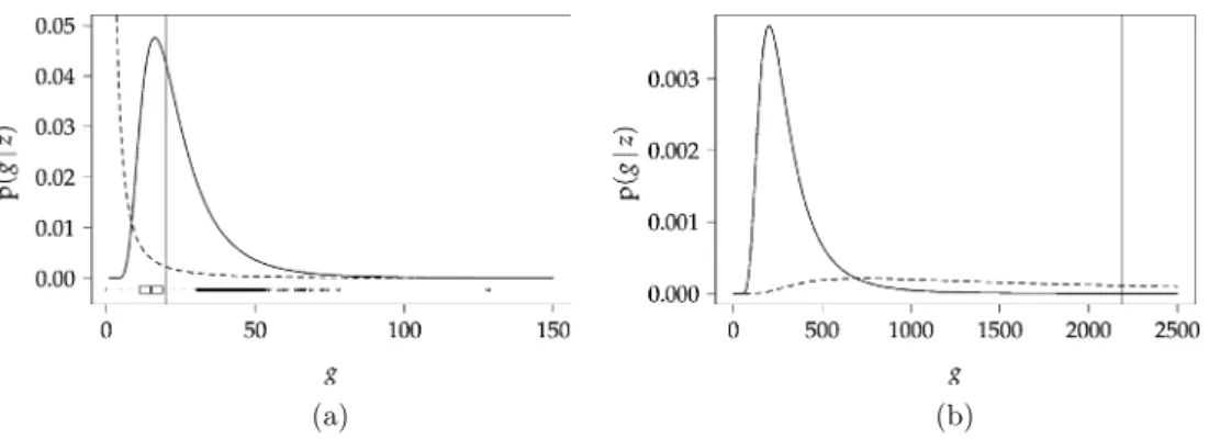
In Figure3, the posterior distributions ofgare com-pared with the underlying conjugate prior distributions (ZS adapted and hyper-g) and local as well as global
EB estimates ofg. The posterior distributions are based on all models and computed using the identity
p(g|z)=
j∈J
p(g|zj,Mj)Pr(Mj|zj).
We clearly see the difference between the two priors re-sulting from the different hyperparameter choices. The fixed choices g=n (BIC) and g=2n are not sup-ported by the data, as all estimates are far below these values. The local EB estimates of g tend to be small, with the posterior mode of g under the hyper-g prior and the global EB estimate having similar values. The posterior mode ofgunder the ZS adapted prior is larger than the other estimates but still much smaller than the fixed choices.
4.2 Shrinkage of Coefficients
We now consider the MPM model identified in the previous section with either the local EB, hyper-g, or
FIG. 3. Comparison of priors(dashed lines)and posteriors(solid lines)ofgunder the conjugate incomplete inverse-gamma prior with hyper-g(left)and ZS adapted(right)hyperparameter choices. (a)Hyper-gprior and posterior,together with local EB(boxplot for the values at bottom of the plot)and global EB(vertical line)estimates ofg. (b)ZS adapted prior and posterior,together withg=n(vertical line).
hyper-g/n approach, which includes the eight vari-ables x1, x2, x3, x5, x6, x8, x10, and x16. Integrated nested Laplace approximations [Rue, Martino and Chopin (2009)] have been used to fit Bayesian logis-tic regression models under the generalizedg-prior for various values ofgwith the R-INLA package ( www.r-inla.org). The constant c in (7) has been fixed based on the estimate αˆ of α in the null model. Empirical shrinkage is defined as the ratio of the resulting poste-rior mean estimates of the regression coefficients over the corresponding MLEs. Empirical shrinkage can also be computed based on the ratio of the resulting poste-rior variances over the corresponding variances of the MLEs; compare equation (11).
Figure4 shows that there is a good agreement be-tween empirical and theoretical shrinkage g/(g+1) for most regression coefficients, which supports the va-lidity of the approximation (11). The agreement is not so good forx2(Age) and the factor variablex3(Killip class), perhaps because the strong degree of discrimi-nation of these important predictors may affect the va-lidity of the approximation I(α,βj)≈I(α,0) from Section3.1.
4.3 Bootstrap Cross-Validation
To quantify and compare the predictive performance of the TBF methods, we have performed a bootstrap cross-validation study. To reduce computation time, we have used the best 8000 models based on a stochastic model search, as described inSabanés Bové and Held (2011b) with 30,000 iterations, instead of exhaustive evaluation of all models. We have used the area un-der the ROC curve (AUC, measures discrimination), the calibration slope (CS) [Cox(1958), measures cali-bration], and the logarithmic score (LS) (measures both
discrimination and calibration) to quantify the predic-tive performance. SeeGneiting and Raftery(2007) for a theoretical andSteyerberg(2009) for a more practi-cal review of methods to validate and compare proba-bilistic predictions. Both AUC and CS are 1 for perfect discrimination and calibration, respectively. In practi-cal applications they will be typipracti-cally smaller than 1. The LS is defined as−mi=1log{ ˆπiyi(1− ˆπi)1−yi}/m,
where πˆi is the predicted probability of death (yi =
1) for the ith patient in the validation sample, i = 1, . . . , m. The LS is negatively oriented, that is, the smaller, the better.
The apparent performance of the methods using the original sample both for fitting and predicting is well-known to be of little value for estimating the predictive performance for new data. Therefore, we compute an estimate of the out-of-sample performance using boot-strap cross-validation. For each of 1000 bootboot-strap sam-ples, we fit the methods and evaluate the above criteria based on the data not included in the bootstrap sample. We compare our methods with a more traditional AIC-or BIC-based approach fAIC-or (Bayesian) model selection and averaging based on posterior model probabilities proportional to exp(−AICj/2)and exp(−BICj/2),
re-spectively [seeClaeskens and Hjort(2008)], and to the Hu and Johnson (2009) choice g=2n. In addition, we apply a recently developed method for variable se-lection in generalized additive models to our setting [Marra and Wood (2011), Section 2.1]. The method gives component-wise shrinkage of covariate effects included, similar to a Bayesian model average (BMA). Finally, simple backward selection with AIC or BIC has been included as well as just fitting the full model. The average criteria are shown in Table 2. Consid-ering first the logarithmic score as our overall crite-rion, we see that, for any of the four methods to esti-mategbased on TBFs, BMA is better than MPM, and
FIG. 4. Shrinkage of posterior means and variances of regression coefficients under the generalizedg-prior for various values ofg.The posterior distribution has been calculated with theR-INLAsoftware and the empirical shrinkage is plotted against the theoretical shrinkage
g/(g+1).
MPM is better than MAP, and this is also true for AUC. This is not surprising, given the theoretical advantage of BMA over single models concerning prediction. The empirical superiority of MPM over MAP indicates that the theoretical superiority of the MPM approach in the linear model may extend to GLMs. We note that the BMA is also superior in terms of calibration, whereas there is no clear preference for either MAP or MPM in terms of CS. Overall, the local EB approach per-forms best, closely followed by hyper-g/n. We would have expected more similarities between local EB and hyper-g, which is substantially worse, in particular, in terms of calibration. The ZS adapted approach is better than hyper-gin terms of calibration, but slightly worse in terms of discrimination and LS.
Considering the alternatives to the TBF approach, AIC-weighted model selection has a similar perfor-mance to hyper-gand ZS adapted, but is not as good as local EB or hyper-g/n. BIC-weighted model selection and fixinggat 2nperform substantially worse, and so do the two stepwise procedures. Simply using the full model gives reasonable discrimination, but very poor calibration, and so the LS is very poor. Among the alternative methods, the variable selection according
to Marra and Wood(2011) (“GLM Select”) performs best. Its additional flexibility from separate shrinkage of the coefficients leads to a similar performance as our (global shrinkage) MPM model with either local EB or hyper-g/n. However, it is not as good as the BMAs (which also have implicit coefficient-wise shrinkage) with any of our four approaches.
5. DISCUSSION
In this paper we considered test-based Bayes factors derived from the deviance statistic for generalized lin-ear models, emphasizing that the implicitly used prior on the regression coefficients is a generalized g-prior. As with the data-based Bayes factors, estimation ofgis possible and recommended. Local EB estimation of g leads to posterior means of the regression coefficients that correspond to shrinkage estimates from the litera-ture. Alternatively, full Bayes estimation ofgis possi-ble and leads to generalized hyper-gpriors.
In an empirical comparison, the TBFs have been shown to be in good agreement with the correspond-ing DBFs. We developed a bias-correction in the lin-ear model under empirical Bayes which has further
re-TABLE2
GUSTO-I data:Comparison of the predictive performance of variable selection using bootstrap cross-validation of AUC,
Calibration slope(CS),and Logarithmic score(LS)
AUC CS LS Local EB MAP 0.8313 0.8643 0.1874 MPM 0.8322 0.8616 0.1870 BMA 0.8344 0.8864 0.1860 Hyper-g MAP 0.8314 0.8141 0.1880 MPM 0.8322 0.8196 0.1876 BMA 0.8343 0.8406 0.1865 Hyper-g/n MAP 0.8310 0.8558 0.1877 MPM 0.8320 0.8547 0.1872 BMA 0.8345 0.8818 0.1860 ZS adapted MAP 0.8296 0.8396 0.1887 MPM 0.8300 0.8398 0.1885 BMA 0.8343 0.8662 0.1866 AIC MAP 0.8316 0.8208 0.1886 MPM 0.8318 0.8271 0.1884 BMA 0.8339 0.8492 0.1873 BIC MAP 0.8259 0.8415 0.1908 MPM 0.8261 0.8424 0.1907 BMA 0.8313 0.8837 0.1884 Fixedg=2n MAP 0.8250 0.8418 0.1906 MPM 0.8251 0.8426 0.1905 BMA 0.8308 0.8766 0.1881 GLM full 0.8314 0.8108 0.1888 GLM select 0.8330 0.8787 0.1871 Step AIC 0.8314 0.8205 0.1887 Step BIC 0.8285 0.8426 0.1898
duced the error. It will be interesting to develop simi-lar corrections for the fully Bayesian approaches. An-other important area of theoretical research would be to investigate the conditions for optimality of the MPM model in GLMs.
TBFs are applicable in a wider context. In particular, the proposed methodology can be used for function se-lection [Sabanés Bové and Held (2011b)] and can be extended to the Cox proportional hazards model, which we will report elsewhere. Also, regression models for multicategorical data such as the proportional odds model or the multinomial logistic regression model re-turn a deviance, so the TBF approach will be applica-ble in these settings. The same is true for CART mod-els [Gravestock(2014)] and mixed models with fixed (known) random effects variances, where a (marginal) deviance is also available. This is important in our con-text, as it would allow us to combine the spline-based Bayesian model and function selection [Sabanés Bové, Held and Kauermann (2014)] with TBFs. However,
more research on the asymptotic distribution of the de-viance is needed for the application of TBFs to mixed models with unknown variance components.
APPENDIX A: PROOFS FOR SECTION2.2.1
In Section2.2.1we state that the distribution of the deviance converges for n→ ∞ to a noncentral chi-squared distribution withdj degrees of freedom, where
λj =β⊤jIβj,βjβj is the noncentrality parameter. This
is essentially proven by Davidson and Lever (1970), and we briefly show how their Theorem 1 applies here. In their notation the model is parametrized by θ=(θ⊤1, θ2)⊤withθ1=βj being the parameter of
in-terest andθ2=αbeing the nuisance parameter. We test the null hypothesisH0: θ =θ0 =(0⊤, θ2)⊤. We con-sider a sequence of local alternativesθn=(θn1, θ2)with components θ1nk =δk/√n of θn1, where δk =0, k=
1, . . . , dj. It follows that θn→θ0 for n→ ∞. Then Theorem 1 of Davidson and Lever (1970) states that for n→ ∞ the deviance converges in distribution to a noncentral chi-squared distribution with dj degrees
of freedom and noncentrality parameter δ⊤C11(θ0)δ, whereδ=(δ1, . . . , δdj)⊤. HereC11(θ0)is the inverse
of the submatrix corresponding toθ1of the inverse ex-pected Fisher information from one observation, eval-uated atθ =θ0. But we know that the expected Fisher information is block-diagonal for θ =θ0, so C11(θ0) is just the submatrix of the expected Fisher informa-tion from one observainforma-tion. Moreover, for n observa-tions we have Iβ
j,βj =n ·C11(θ0), and combined
with δ=√nβj, we obtain the noncentrality parame-terλj =β⊤jIβj,βjβj.
In order to derive the prior distribution forλj based
on the generalizedg-prior (8) for βj as stated in Sec-tion2.2.2, first note that the generalizedg-prior corre-sponds to ˜ βj =Iβ1/2 j,βj/ √g βj ∼Ndj(0,Idj), where I1/2
βj,βj is the upper-triangular Cholesky root of
Iβ
j,βj. Hence, β˜
⊤
jβ˜j ∼χ2(dj), which is a G(dj/2,
1/2) distribution. Expanding the quadratic form, we obtain ˜ β⊤j β˜j =1/√gβ⊤jIβ⊤/2 j,βjI 1/2 βj,βjβj1/√g =1/gβ⊤j Iβ j,βjβj =λj/g and, finally,λj =g·λj/g∼G(dj/2,1/(2g)).
APPENDIX B: PROOFS FOR SECTION3.2
For ease of notation we drop the indexj of the al-ternative model and simply denote the deviance withz, the associated degrees of freedom withd, while TBF denotes the corresponding TBF with respect to the null model.
For the bounds mentioned in Section3.2usually the minimum Bayes factor in favor of the null hypothe-sis is considered, which is mTBF−1 in our notation. Let theP-value bep=1−Fχ2(d)(z), where Fχ2(d)is the cumulative distribution function of the chi-squared distribution withd degrees of freedom. The proofs are adapted fromMalaguerra(2012):
1. Letd=1 andz > d=1. Letq=−1(1−p/2) be the corresponding quantile of the standard nor-mal distribution with cumulative distribution func-tion. We haveq2=z since a squared standard nor-mal random variable is χ2(1)-distributed and, hence, mTBF−1=z1/2exp(−z/2)exp(1/2)=qexp(−q2/2)· √
e, which is the required result fromBerger and Sellke (1987).
2. Letd=2 andz > d=2. Due to Fχ2(2)(z)=1− exp(−z/2), we havep=exp(−z/2)orz= −2 log(p), such that z >2 is equivalent to p <1/e. Moreover, mTBF−1 = (2/z)−1exp(−(z−2)/2) = −eplog(p), which is the required result from Sellke, Bayarri and Berger(2001).
3. The universal bound fromEdwards, Lindman and Savage (1963) that we want to reach is exp(−q2/2), hereq =−1(1−p). We have to show that ford→ ∞ and fixed P-value, the ratio of mTBF−1 and this universal bound is 1. With d → ∞ we have (z − d)/√2d ∼a N(0,1) and, hence, z≈d +√2dq. Plug-ging this in (13), we obtain
mTBF−1 exp(−q2/2) ≈ d √ 2dq+d −d/2 exp − d 2q+q 2/2
=exp−aq+a2log(1+q/a)+q2/2 witha=√d/2. Now for larged the termq/ais small and, hence, we can apply a second-order Taylor expan-sion of log(1+x) aroundx=0, giving log(1+x)≈ x−x2/2, and we obtain mTBF−1 exp(−q2/2)≈exp −aq+a2 q a − q2 2a2 +q 2 2 =exp(0)=1, which proves the statement.
ACKNOWLEDGMENTS
We thank Kerry L. Lee and Ewout W. Steyerberg for permission to use the GUSTO-I data set. We are also grateful to Rafael Sauter for help with the R-INLA software in Section 4.2and to Manuela Ott for proof-reading the final manuscript. We finally acknowledge helpful comments by two referees on an earlier version of this article.
REFERENCES
BARBIERI, M. M. and BERGER, J. O. (2004). Optimal predictive model selection.Ann.Statist.32870–897.MR2065192
BAYARRI, M. J., BERGER, J. O., FORTE, A. and GARCÍA -DONATO, G. (2012). Criteria for Bayesian model choice with application to variable selection. Ann.Statist.40 1550–1577.
MR3015035
BERGER, J. O. and PERICCHI, L. R. (2001). Objective Bayesian methods for model selection: Introduction and comparison. In
Model Selection (P. Lahiri, eds.). Institute of Mathematical Statistics Lecture Notes—Monograph Series38135–207. IMS, Beachwood, OH.MR2000753
BERGER, J. O. and SELLKE, T. (1987). Testing a point null hy-pothesis: Irreconcilability of p-values and evidence. J. Amer.
Statist.Assoc.82112–139.MR0883340
CLAESKENS, G. and HJORT, N. L. (2008). Model Selection
and Model Averaging. Cambridge Univ. Press, Cambridge.
MR2431297
COPAS, J. B. (1983). Regression, prediction and shrinkage.J.R.
Stat.Soc.Ser.B.Stat.Methodol.45311–354.MR0737642
COPAS, J. B. (1997). Using regression models for prediction: Shrinkage and regression to the mean.Stat.Methods Med.Res.
6167–183.
COX, D. R. (1958). Two further applications of a model for binary regression.Biometrika45562–565.
CUI, W. and GEORGE, E. I. (2008). Empirical Bayes vs. fully Bayes variable selection.J.Statist.Plann.Inference138888– 900.MR2416869
DAVIDSON, R. R. and LEVER, W. E. (1970). The limiting dis-tribution of the likelihood ratio statistic under a class of local alternatives.Sankhy¯a Ser.A32209–224.MR0297050
EDWARDS, W., LINDMAN, H. and SAVAGE, L. J. (1963).
Bayesian statistical inference for psychological research. Psy-chological Review70193–242.
FERNÁNDEZ, C., LEY, E. and STEEL, M. F. J. (2001). Benchmark priors for Bayesian model averaging.J.Econometrics100381– 427.MR1820410
FOSTER, D. P. and GEORGE, E. I. (1994). The risk inflation criterion for multiple regression. Ann.Statist.22 1947–1975.
MR1329177
GEISSER, S. (1984). On prior distributions for binary trials.Amer.
Statist.38244–251.MR0770258
GEORGE, E. I. and FOSTER, D. P. (2000). Calibration and empirical Bayes variable selection. Biometrika 87 731–747.
MR1813972
GNEITING, T. and RAFTERY, A. E. (2007). Strictly proper scoring rules, prediction, and estimation. J.Amer. Statist. Assoc. 102
GOODMAN, S. N. (1999a). Toward evidence-based medical statis-tics. 1: TheP-value fallacy.Annals of Internal Medicine130
995–1004.
GOODMAN, S. N. (1999b). Toward evidence-based medical statis-tics. 2: The Bayes factor.Annals of Internal Medicine1301005– 1013.
GRAVESTOCK, I. (2014). Bayesian tree models priors and poste-rior approximations. Master’s thesis, Univ. Zurich.
HELD, L. (2010). A nomogram forP-values.BMC Medical Re-search Methodology1021.
HJORT, N. L. and CLAESKENS, G. (2003). Frequentist model average estimators. J. Amer. Statist. Assoc. 98 879–899.
MR2041481
HU, J. and JOHNSON, V. E. (2009). Bayesian model selection us-ing test statistics.J.R.Stat.Soc.Ser.B.Stat.Methodol.71143– 158.MR2655527
JOHNSON, V. E. (2005). Bayes factors based on test statistics.J.R.
Stat.Soc.Ser.B.Stat.Methodol.67689–701.MR2210687
JOHNSON, V. E. (2008). Properties of Bayes factors based on test statistics.Scand.J.Stat.35354–368.MR2418746
KASS, R. E. and WASSERMAN, L. (1995). A reference Bayesian test for nested hypotheses and its relationship to the Schwarz criterion.J.Amer.Statist.Assoc.90928–934.MR1354008
LAWLESS, J. F. and SINGHAL, K. (1978). Efficient screening of nonnormal regression models.Biometrics34318–327. LEE, K. L., WOODLIEF, L. H., TOPOL, E. J., WEAVER, W. D.,
BETRIU, A., COL, J., SIMOONS, M., AYLWARD, P., VAN DE
WERF, F. and CALIFF, R. M. (1995). Predictors of 30-day mor-tality in the era of reperfusion for acute myocardial infarction: Results from an international trial of 41,021 patients. Circula-tion911659–1668.
LIANG, F., PAULO, R., MOLINA, G., CLYDE, M. A. and BERGER, J. O. (2008). Mixtures of g priors for Bayesian variable selection. J. Amer. Statist. Assoc. 103 410–423.
MR2420243
LINDLEY, D. V. (1957). A statistical paradox.Biometrika44187– 192.
MALAGUERRA, A. (2012). Bayesian variable selection based on test statistics. Master’s thesis, Univ. Zurich.
MARRA, G. and WOOD, S. N. (2011). Practical variable selection for generalized additive models.Comput.Statist.Data Anal.55
2372–2387.MR2786996
NELDER, J. A. and WEDDERBURN, R. W. M. (1972). General-ized linear models.J.Roy.Statist.Soc.Ser.A135370–384. RUE, H., MARTINO, S. and CHOPIN, N. (2009). Approximate
Bayesian inference for latent Gaussian models using integrated nested Laplace approximations (with discussion).J.Roy.Statist.
Soc.Ser.B71319–392.
SABANÉS BOVÉ, D. and HELD, L. (2011a). Hyper-g priors for generalized linear models. Bayesian Anal. 6 387–410.
MR2843537
SABANÉSBOVÉ, D. and HELD, L. (2011b). Bayesian fractional polynomials.Stat.Comput.21309–324.MR2806611
SABANÉS BOVÉ, D., HELD, L. and KAUERMANN, G. (2014). Mixtures of g-priors for generalised additive model selec-tion with penalised splines. J. Comput. Graph. Statist.DOI:
10.1080/10618600.2014.912136.
SCOTT, J. G. and BERGER, J. O. (2010). Bayes and empirical-Bayes multiplicity adjustment in the variable-selection problem.
Ann.Statist.382587–2619.MR2722450
SELLKE, T., BAYARRI, M. J. and BERGER, J. O. (2001). Cali-bration ofp-values for testing precise null hypotheses.Amer.
Statist.5562–71.MR1818723
STEYERBERG, E. (2009).Clinical Prediction Models. Springer, New York.
VANHOUWELINGEN, J. C. and LECESSIE, S. (1990). Predictive value of statistical models.Stat.Med.91303–1325.
ZELLNER, A. (1986). On assessing prior distributions and
Bayesian regression analysis with g-prior distributions. In
Bayesian Inference and Decision Techniques(P. K. Goel and A. Zellner, eds.).Stud.Bayesian Econometrics Statist.6233– 243. North-Holland, Amsterdam.MR0881437
ZELLNER, A. and SIOW, A. (1980). Posterior odds ratios for selected regression hypotheses. In Bayesian Statistics: Pro-ceedings of the First International Meeting Held in Valen-cia (J. M. Bernardo, M. H. DeGroot, D. V. Lindley and A. F. M. Smith, eds.) 585–603. Univ. Valencia Press, Valencia.