Queen’s Economics Department Working Paper No. 1135 (Revised)
Wild Bootstrap Tests for IV Regression
Russell Davidson
McGill University
James G. MacKinnon
Queen’s University
Department of Economics
Queen’s University
94 University Avenue
Kingston, Ontario, Canada
K7L 3N6
Wild Bootstrap Tests for IV Regression
Russell Davidson
GREQAMCentre de la Vieille Charit´e 2 rue de la Charit´e
13236 Marseille cedex 02, France
Department of Economics McGill University Montreal, Quebec, Canada
H3A 2T7 email: [email protected] and
James G. MacKinnon
Department of Economics Queen’s University Kingston, Ontario, CanadaK7L 3N6
email: [email protected]
Abstract
We propose a wild bootstrap procedure for linear regression models estimated by instrumental variables. Like other bootstrap procedures that we have proposed else-where, it uses efficient estimates of the reduced-form equation(s). Unlike them, it takes account of possible heteroskedasticity of unknown form. We apply this procedure to
ttests, including heteroskedasticity-robustttests, and to the Anderson-Rubin test. We provide simulation evidence that it works far better than older methods, such as the pairs bootstrap. We also show how to obtain reliable confidence intervals by inverting bootstrap tests. An empirical example illustrates the utility of these procedures.
Keywords: Instrumental variables estimation, two-stage least squares, weak
instru-ments, wild bootstrap, pairs bootstrap, residual bootstrap, confidence intervals, Anderson-Rubin test
JEL codes: C12, C15, C30
This research was supported, in part, by grants from the Social Sciences and Humanities Research Council of Canada, the Canada Research Chairs program (Chair in Economics, McGill University), and the Fonds Qu´eb´ecois de Recherche sur la Soci´et´e et la Culture. We are grateful to Arthur Sweetman for a valuable suggestion and to two referees and an associate editor for very helpful comments.
1. Introduction
It is often difficult to make reliable inferences from regressions estimated using instru-mental variables. This is especially true when the instruments are weak. There is an enormous literature on this subject, much of it quite recent. Most of the papers focus on the case in which there is just one endogenous variable on the right-hand side of the regression, and the problem is to test a hypothesis about the coefficient of that variable. In this paper, we also focus on this case, but, in addition, we discuss confidence intervals, and we allow the number of endogenous variables to exceed two. One way to obtain reliable inferences is to use statistics with better properties than those of the usual IV t statistic. These include the famous Anderson-Rubin, or AR, statistic proposed in Anderson and Rubin (1949) and extended in Dufour and Taamouti (2005, 2007), the Lagrange Multiplier, or K, statistic proposed in Kleibergen (2002), and the conditional likelihood ratio, or CLR, test proposed in Moreira (2003). A detailed analysis of several tests is found in Andrews, Moreira, and Stock (2006). A second way to obtain reliable inferences is to use the bootstrap. This approach has been much less popular, probably because the simplest bootstrap methods for this problem do not work very well. See, for example, Flores-Lagunes (2007). However, the more sophisticated bootstrap methods recently proposed in Davidson and MacKinnon (2008) work very much better than traditional bootstrap procedures, even when they are combined with the usual t statistic.
One advantage of the t statistic over the AR, K, and CLR statistics is that it can easily be modified to be asymptotically valid in the presence of heteroskedasticity of unknown form. But existing procedures for bootstrapping IV t statistics either are not valid in this case or work badly in general. The main contribution of this paper is to propose a new bootstrap data generating process (DGP) which is valid under heteroskedasticity of unknown form and works well in finite samples even when the instruments are quite weak. This is a wild bootstrap version of one of the methods proposed in Davidson and MacKinnon (2008). Using this bootstrap method together with a heteroskedasticity-robust t statistic generally seems to work remarkably well, even though it is not asymptotically valid under weak instrument asymptotics. The method can also be used with other test statistics that are not heteroskedasticity-robust. It seems to work particularly well when used with the AR statistic, probably because the resulting test is asymptotically valid under weak instrument asymptotics. In the next section, we discuss six bootstrap methods that can be applied to test statistics for the coefficient of the single right-hand side endogenous variable in a linear regression model estimated by IV. Three of these have been available for some time, two were proposed in Davidson and MacKinnon (2008), and one is a new procedure based on the wild bootstrap. In Section 3, we discuss the asymptotic validity of several tests based on this new wild bootstrap method. In Section 4, we investigate the finite-sample performance of the new bootstrap method and some existing ones by simulation. Our simulation results are quite extensive and are presented graphically.
In Section 5, we briefly discuss the more general case in which there are two or more endogenous variables on the right-hand side. In Section 6, we discuss how to obtain confidence intervals by inverting bootstrap tests. Finally, in Section 7, we present an empirical application that involves estimation of the return to schooling.
2. Bootstrap Methods for IV Regression
In most of this paper, we deal with the two-equation model
y1 =βy2+Zγ+u1 (1)
y2 =Wπ+u2. (2)
Here y1 andy2 are n--vectors of observations on endogenous variables, Z is an n×k
matrix of observations on exogenous variables, and W is ann×l matrix of exogenous instruments with the property that S(Z), the subspace spanned by the columns of Z, lies in S(W), the subspace spanned by the columns ofW. Equation (1) is a structural equation, and equation (2) is a reduced-form equation. Observations are indexed by i, so that, for example, y1i denotes theith element of y1.
We assume that l > k. This means that the model is either just identified or over-identified. The disturbances are assumed to be serially uncorrelated. When they are homoskedastic, they have a contemporaneous covariance matrix
Σ ≡ σ2 1 ρσ1σ2 ρσ1σ2 σ22 .
However, we will often allow them to be heteroskedastic with unknown (but bounded) variances σ2
1i and σ 2
2i and correlation coefficient ρi that may depend on Wi, the row vector of instrumental variables for observation i.
The usual t statistic for β =β0 can be written as
ts( ˆβ, β0) = ˆ β−β0 ˆ σ1||PWy2−PZy2|| , (3)
where ˆβ is the generalized IV, or 2SLS, estimate of β, PW and PZ are the matrices that project orthogonally on to the subspaces S(W) and S(Z), respectively, and || · || denotes the Euclidean length of a vector. In equation (3),
ˆ σ1 = 1 −nu1ˆ ⊤ ˆ u1 1/2 =−1n(y1−βˆy2−Zγˆ)⊤ (y1−βˆy2−Zγˆ) 1/2 (4) is the usual 2SLS estimate of σ1. Here ˆγ denotes the IV estimate ofγ, and ˆu1 is the usual vector of IV residuals. Many regression packages divide by n−k−1 instead of by n. Since ˆσ1 as defined in (4) is not necessarily biased downwards, we do not do so.
When homoskedasticity is not assumed, the usual t statistic (3) should be replaced by the heteroskedasticity-robust t statistic
th( ˆβ, β0) = ˆ β −β0 sh( ˆβ) , (5) where sh( ˆβ)≡ Pn i=1uˆ 2 1i(PWy2−PZy2)2i 1/2 PWy2−PZy2 2 . (6)
Here (PWy2−PZy2)idenotes theith element of the vectorPWy2−PZy2. Expression
(6) is what most regression packages routinely print as a heteroskedasticity-consistent standard error for ˆβ. It is evidently the square root of a sandwich variance estimate. The basic idea of bootstrap testing is to compare the observed value of some test statistic, say ˆτ, with the empirical distribution of a number of bootstrap test statistics, say τ∗
j, for j = 1, . . . , B, where B is the number of bootstrap replications. The bootstrap statistics are generated using the bootstrap DGP, which must satisfy the null hypothesis tested by the bootstrap statistics. When α is the level of the test, it is desirable that α(B+ 1) should be an integer, and a commonly used value of B is 999. See Davidson and MacKinnon (2000) for more on how to choose B appropriately. If we are prepared to assume thatτ is symmetrically distributed around the origin, then it is reasonable to use the symmetric bootstrapP value
ˆ p∗s(ˆτ) = 1 B B X j=1 I |τj∗|>|τˆ| . (7)
We reject the null hypothesis whenever ˆp∗
s(ˆτ)< α.
For test statistics that are always positive, such as the AR andK statistics that will be discussed in the next section, we can use (7) without taking absolute values, and this is really the only sensible way to proceed. In the case of IV t statistics, however, the probability of rejecting in one direction can be very much greater than the probability of rejecting in the other, because ˆβ is often biased. In such cases, we can use the equal-tail bootstrap P value
ˆ p∗et(ˆτ) = 2 min 1 B B X j=1 I(τj∗ ≤τˆ), 1 B B X j=1 I(τj∗ >τˆ) . (8)
Here we actually perform two tests, one against values in the lower tail of the distribu-tion and the other against values in the upper tail, and reject if either of them yields a bootstrap P value less than α/2.
Bootstrap testing can be expected to work well when the quantity bootstrapped is approximately pivotal, that is, when its distribution changes little as the DGP varies
within the limits of the null hypothesis under test. In the ideal case in which a test statistic is exactly pivotal and B is chosen properly, bootstrap tests are exact. See, for instance, Horowitz (2001) for a clear exposition.
The choice of the DGP used to generate the bootstrap samples is critical, and it can dramatically affect the properties of bootstrap tests. In the remainder of this section, we discuss six different bootstrap DGPs for tests of β = β0 in the IV regression
model given by (1) and (2). Three of these have been around for some time, but they often work badly. Two were proposed in Davidson and MacKinnon (2008), and they generally work very well under homoskedasticity. The last one is new. It is a wild bootstrap test that takes account of heteroskedasticity of unknown form.
The oldest and best-known method for bootstrapping the test statistics (3) and (5) is to use the pairs bootstrap, which was originally proposed in Freedman (1981) and applied to 2SLS regression in Freedman (1984). The idea is to resample the rows of the matrix
[y1 y2 W]. (9)
For the pairs bootstrap, the ith
row of each bootstrap sample is simply one of the rows of the matrix (9), chosen at random with probability 1/n. Other variants of the pairs bootstrap have been proposed for this problem. In particular, Moreira, Porter, and Suarez (2005) propose a variant that seems more complicated, because it involves estimating the model, but actually yields identical results when applied to both ordinary and heteroskedasticity-robust t statistics. Flores-Lagunes (2007) proposes another variant that yields results very similar, but not identical, to those from the ordinary pairs bootstrap.
Because the pairs bootstrap DGP does not impose the null hypothesis, the bootstrap t statistics must be computed as
t( ˆβj∗,β) =ˆ ˆ β∗ j −βˆ se( ˆβ∗ j) . (10) Here ˆβ∗
j is the IV estimate of β from the j
th
bootstrap sample, and se( ˆβ∗
j) is the standard error of ˆβ∗
j, calculated by whatever method is used for the standard error of ˆ
β in the t statistic that is being bootstrapped. If we used β0 in place of ˆβ in (10), we
would be testing a hypothesis that was not true of the bootstrap DGP.
The pairs bootstrap is fully nonparametric and is valid in the presence of heteroskedas-ticity of unknown form, but, as we shall see in Section 4, it has little else to recommend it. The other bootstrap methods that we consider are semiparametric and require esti-mation of the model given by (1) and (2). We consider a number of ways of estimating this model and constructing bootstrap DGPs.
The least efficient way to estimate the model is to use OLS on the reduced-form equation (2) and IV on the structural equation (1), without imposing the restriction that β = β0. This yields estimates ˆβ, ˆγ, and ˆπ, a vector of IV residuals ˆu1, and a
vector of OLS residuals ˆu2. Using these estimates, we can easily construct the DGP
for the unrestricted residual bootstrap, or UR bootstrap. The UR bootstrap DGP can be written as y∗ i1 = ˆβy ∗ 2i+Ziγˆ + ˆu∗1i (11) y∗2i =Wiπˆ + ˆu∗2i, (12) where ˆ u∗ 1i ˆ u∗ 2i ∼EDF uˆ1i n/(n−l)1/2 ˆ u2i ! . (13)
Equations (11) and (12) are simply the structural and reduced-form equations evalu-ated at the unrestricted estimates. Note that we could omit Ziγˆ from equation (11), since the t statistics are invariant to the true value ofγ.
According to (13), the bootstrap disturbances are drawn in pairs from the joint empiri-cal distribution of the unrestricted residuals, with the residuals from the reduced-form equation rescaled so as to have variance equal to the OLS variance estimate. This rescaling is not essential. It would also be possible to rescale the residuals from the structural equation, but it is unclear what benefit might result. The bootstrap DGP given by (11), (12), and (13) ensures that, asymptotically, the joint distribution of the bootstrap disturbances is the same as the joint distribution of the actual disturbances if the model is correctly specified and the disturbances are homoskedastic.
Since the UR bootstrap DGP does not impose the null hypothesis, the bootstrap test statistics must be calculated in the same way as for the pairs bootstrap, using equation (10), so as to avoid testing a hypothesis that is not true of the bootstrap DGP. Whenever possible, it is desirable to impose the null hypothesis of interest on the bootstrap DGP. This is because imposing a (true) restriction makes estimation more efficient, and using more efficient estimates in the bootstrap DGP should reduce the error in rejection probability (ERP) associated with the bootstrap test. In some cases, it can even improve the rate at which the ERP shrinks as the sample size increases; see Davidson and MacKinnon (1999). All of the remaining bootstrap methods that we discuss impose the null hypothesis.
The DGP for therestricted residual bootstrap, orRR bootstrap, is very similar to the one for the UR bootstrap, but it imposes the null hypothesis on both the structural equation and the bootstrap disturbances. Without loss of generality, we suppose that β0 = 0. Under this null hypothesis, equation (1) becomes a regression of y1 on Z,
which yields residuals ˜u1. We therefore replace equation (11) by
y∗i1 = ˜u
∗
1i, (14)
since the value of γ does not matter. Equation (12) is used unchanged, and equation (13) is replaced by
˜ u∗ 1i ˆ u∗ 2i ∼EDF n/(n−k) 1/2 ˜ u1i n/(n−l)1/2 ˆ u2i ! . Since ˜u1i is just an OLS residual, it makes sense to rescale it here.
As we shall see in Section 4, the RR bootstrap outperforms the pairs and UR boot-straps, but, like them, it does not work at all well when the instruments are weak. The problem is that ˆπ is not an efficient estimator of π, and, when the instruments are weak, ˆπ may be very inefficient indeed. Therefore, Davidson and MacKinnon (2008) suggested using a more efficient estimator, which was also used by Kleibergen (2002) in constructing the K statistic. This estimator is asymptotically equivalent to the ones that would be obtained by using either 3SLS or FIML on the system consisting of equations (1) and (2). It may be obtained by running the regression
y2 =Wπ+δMZy1+ residuals. (15)
This is just the reduced-form equation (2) augmented by the residuals from restricted estimation of the structural equation (1). It yields estimates ˜π and ˜δ and residuals
˜
u2 ≡y2−Wπ.˜
These are not the OLS residuals from (15), which would be too small, but the OLS residuals plus ˜δMZy1.
This procedure provides all the ingredients for what Davidson and MacKinnon (2008) call the restricted efficient residual bootstrap, or RE bootstrap. The DGP uses equa-tion (14) as the structural equaequa-tion and
y2∗i=Wiπ˜ + ˜u ∗
2i (16)
as the reduced-form equation, and the bootstrap disturbances are generated by ˜ u∗ 1i ˜ u∗ 2i ∼EDF n/(n−k) 1/2 ˜ u1i n/(n−l)1/2 ˜ u2i ! . (17)
Here the residuals are rescaled in exactly the same way as for the RR bootstrap. This rescaling, which is optional, should have only a slight effect unless k and/or l is large relative to n.
One of several possible measures of how strong the instruments are is theconcentration parameter, which can be written as
a2 ≡ 1 σ2
2
Evidently, the concentration parameter is large when the ratio of the error variance in the reduced-form equation to the variance explained by the part of the instruments that is orthogonal to the exogenous variables in the structural equation is small. We can estimate a2
using either OLS estimates of equation (2) or the more efficient estimates ˜
π1 and ˜σ obtained from regression (15). However, both estimates are biased upwards,
because of the tendency for OLS estimates to fit too well. Davidson and MacKinnon (2008) therefore proposes the bias-corrected estimator
˜
a2BC ≡max 0,˜a 2
−(l−k)(1−ρ˜2) ,
where ˜ρ is the sample correlation between the elements of ˜u1 and ˜u2. The
bias-corrected estimator can be used in a modified version of the RE bootstrap, called the REC bootstrap by Davidson and MacKinnon. It uses
y2∗i =W1iπ¨1+ ˜u
∗
2i, where ¨π1 = (˜aBC/˜a) ˜π1,
instead of equation (16) as the reduced-form equation in the bootstrap DGP. The boot-strap disturbances are still generated by (17). Simulation experiments not reported here, in addition to those in the original paper, show that, when applied tot statistics, the performance of the RE and REC bootstraps tends to be very similar. Either one of them may perform better in any particular case, but neither appears to be superior overall. We therefore do not discuss the REC bootstrap further.
As shown in Davidson and MacKinnon (2008), and as we will see in Section 4, the RE bootstrap, based on efficient estimates of the reduced form, generally works very much better than earlier methods. However, like the RR and UR bootstraps (and unlike the pairs bootstrap), it takes no account of possible heteroskedasticity. We now propose a new bootstrap method which does so. It is a wild bootstrap version of the RE bootstrap.
The wild bootstrap was originally proposed in Wu (1986) in the context of OLS re-gression. It can be generalized quite easily to the IV case studied in this paper. The idea of the wild bootstrap is to use for the bootstrap disturbance(s) associated with theith
observation the actual residual(s) for that observation, possibly transformed in some way, and multiplied by a random variable, independent of the data, with mean 0 and variance 1. Often, a binary random variable is used for this purpose. We propose the wild restricted efficient residual bootstrap, or WRE bootstrap. The DGP uses (14) and (16) as the structural and reduced form equations, respectively, with
˜ u∗ 1i ˜ u∗ 2i = " n/(n−k)1/2 ˜ u1ivi∗ n/(n−l)1/2 ˜ u2ivi∗ # , (19) where v∗
i is a random variable that has mean 0 and variance 1. Until recently, the most popular choice for v∗
i has been v∗ i = ( −(√5−1)/2 with probability (√5 + 1)/(2√5); (√5 + 1)/2 with probability (√5−1)/(2√5). (20)
However, Davidson and Flachaire (2008) have shown that, when the disturbances are not too asymmetric, it is better to use the Rademacher distribution, according to which
vi∗ = 1 with probability 12; vi∗ =−1 with probability 12. (21) Notice that, in equation (19), both rescaled residuals are multiplied by the same value of v∗
i. This preserves the correlation between the two disturbances, at least when they are symmetrically distributed. Using the Rademacher distribution (21) imposes symmetry on the bivariate distribution of the bootstrap disturbances, and this may affect the correlation when they are not actually symmetric.
In the experiments reported in the next section, we used (21) rather than (20). We did so because all of the disturbances were symmetric, and there is no advantage to using (20) in that case. Investigating asymmetric disturbances would have substantially increased the scope of the experiments. Of course, applied workers may well want to use (21) instead of, or in addition to, (20). In the empirical example of Section 7, we employ both methods and find that they yield very similar results.
There is a good deal of evidence that the wild bootstrap works reasonably well for univariate regression models, even when there is quite severe heteroskedasticity. See, among others, Gon¸calves and Kilian (2004) and MacKinnon (2006). Although the wild bootstrap cannot be expected to work quite as well as a comparable residual bootstrap method when the disturbances are actually homoskedastic, the cost of insuring against heteroskedasticity generally seems to be very small; see Section 4.
Of course, it is straightforward to create wild bootstrap versions of the RR and REC bootstraps that are analogous to the WRE bootstrap. In our simulation experiments, we studied these methods, which it is natural to call the WRR and WREC bootstraps, respectively. However, we do not report results for either of them. The performance of WRR is very similar to that of RR when the disturbances are homoskedastic, and the performance of WREC is generally quite similar to that of WRE.
3. Asymptotic Validity of Wild Bootstrap Tests
In this section, we sketch a proof of the asymptotic validity of the AR test with weak instruments and heteroskedasticity of unknown form when it is bootstrapped using the WRE bootstrap. In addition, we show that both t tests and the K test are not asymptotically valid in this case. In contrast, all four tests are asymptotically valid with strong instruments and the WRE bootstrap.
A bootstrap test is said to be asymptotically valid if the rejection probability under the null hypothesis tends to the nominal level of the test as the sample size tends to infinity. Normally, this means that the limiting distribution of the bootstrap statistic is the same as that of the statistic itself. Whether or not a bootstrap test is asymp-totically valid depends on the null hypothesis under test, on the test statistic that is bootstrapped, on the bootstrap DGP, and on the asymptotic construction used to compute the limiting distribution.
There are two distinct ways in which a bootstrap test can be shown to be asymptot-ically valid. The first is to show that the test statistic is asymptotasymptot-ically pivotal with respect to the null hypothesis. In that case, the limiting distribution of the statistic is the same under any DGP satisfying the null. The second is to show that the boot-strap DGP converges under the null in an appropriate sense to the true DGP. Either of these conditions allows us to conclude that the (random) distribution of the bootstrap statistic converges to the limiting distribution of the statistic generated by the true DGP. If both conditions are satisfied, then the bootstrap test normally benefits from an asymptotic refinement, a result first shown in Beran (1988).
We consider four possible test statistics: ts, th, the Anderson-Rubin statistic AR, and
the Lagrange Multiplier statisticK of Kleibergen (2002). We consider only the WRE bootstrap DGP, because it satisfies the null hypothesis whether or not heteroskedastic-ity is present, and because it is the focus of this paper. We make use of two asymptotic constructions: the conventional one, in which the instruments are “strong”, and the weak-instrument construction of Staiger and Stock (1997).
The homoskedastic case has been dealt with in Davidson and MacKinnon (2008). With strong instruments, AR is pivotal, and the other three test statistics are asymptoti-cally pivotal. With weak instruments, AR is pivotal, and K is asymptotically pivotal, but the t statistics have neither property, because their limiting distributions depend nontrivially on the parameters a and ρ used in weak-instrument asymptotics. It is easy to see that, with heteroskedasticity and strong instruments, only th is
asymptot-ically pivotal, because the three other statistics make use, explicitly or implicitly, of a variance estimator that is not robust to heteroskedasticity. With heteroskedasticity and weak instruments, none of the statistics is asymptotically pivotal, because th is
not asymptotically pivotal even under homoskedasticity.
In the presence of heteroskedasticity, all we can claim so far is thatth gives an
asymp-totically valid bootstrap test with strong instruments. However, the fact that the WRE DGP mimics the true DGP even with heteroskedasticity suggests that it may yield asymptotically valid tests with other statistics. In the remainder of this section, we show that, when the instruments are strong, all four WRE bootstrap tests are asymptotically valid, but, when the instruments are weak, only AR is.
The proof makes use of an old result, restated in Davidson and MacKinnon (2008), according to which the test statisticsts, K, and AR can be expressed as deterministic
functions of six quadratic forms, namely yi⊤P yj, for i, j = 1,2, where the orthogonal projection matrix P is eitherMW or PV ≡PW −PZ. Since all four of the statistics are homogeneous of degree 0 with respect to both y1 and y2 separately, we can,
without loss of generality, restrict attention to the DGP specified by (1) and (2) with any suitable scaling of the endogenous variables. Further, when β = 0, yi⊤
MWyj = ui⊤MWuj, for i, j = 1,2, and y1⊤PVy1 =u1⊤PVu1.
We focus initially on the AR statistic, which is simply the F statistic for π2 = 0 in
the regression
where Z and W2 span the same subspace asW. It can be written as AR = n−l l−k (y1−β0y2)⊤PV(y1−β0y2) (y1−β0y2)⊤MW(y1−β0y2) = n−l l−k u1⊤PVu1 u1⊤MWu1 . (23)
We need to show that, with weak instruments and heteroskedasticity, the quadratic formsu1⊤PVu1 andu1⊤MWu1have the same asymptotic distributions as their analogs
under the WRE bootstrap.
Let V be an n×(l−k) matrix with orthonormal columns such that V⊤V =nIl−k, where the matrix that projects orthogonally on to S(V) is PV. Let element i of the
vector u1 be ui =σiwi, where the wi are homoskedastic with mean 0 and variance 1.
Then, letting Vi denote the ith
row ofV, we have n−1/2
V⊤u1 =n−1/2Pni=1Vi⊤σiwi.
Under standard regularity conditions, the limiting distribution of this expression is given by a central limit theorem, and it is multivariate normal with expectation zero and asymptotic covariance matrix
plim n→∞ 1 −n n X i=1 σ2iVi⊤Vi. (24)
Now consider the wild bootstrap analog of the sample quantity n−1/2
V⊤u1. This
means replacing the vector u1 by a vector u∗1 with element i given by σiw˜iv
∗
i, where ˜
ui =σiwi, and the˜ v∗
i are IID with expectation 0 and variance 1. The sumn −1/2 V⊤u1 is thus replaced by n−1/2V⊤u∗1 =n −1/2X i Vi⊤σiw˜iv ∗ i a =n−1/2X i Vi⊤σiwiv ∗ i. (25)
The asymptotic equality here follows from the fact that ˜wi tends to wi by the consis-tency of the estimates under the null hypothesis. Conditional on the wi, the limiting distribution of the rightmost expression in (25) follows from a central limit theorem. Because Var(v∗
i) = 1, this limiting distribution is normal with expectation zero and asymptotic covariance matrix
plim n→∞ 1 −n n X i=1 σ2 iw 2 iVi⊤Vi. (26)
Since Var(wi) = 1, the unconditional probability limit of this covariance matrix is, by a law of large numbers, just expression (24).
Now consider the quadratic form u1 ⊤ PVu1 =n −1 u1 ⊤ V V⊤u1 = n −1/2 V⊤u1 ⊤ n−1/2 V⊤u1 , which depends solely on the vector n−1/2
V⊤u1. We have shown that the asymptotic
weak or strong instruments. Thus the limiting distribution of the numerator of the AR statistic (26) is unchanged under the WRE bootstrap.
A different argument is needed for the denominator of the AR statistic, because the matrix MW has rank n−l, and so no limiting matrix analogous to (24) exists. By a law of large numbers,
n−1 u1 ⊤ u1 =−1n n X i=1 σ2 iw 2 i →p lim n→∞ 1 −n n X i=1 σ2 i ≡σ¯ 2 ,
where we can readily assume that the last limit exists. Since u1⊤PWu1 = Op(1) as
n→ ∞, we see that the probability limit ofn−1
u1⊤MWu1 is just ¯σ2. If we once more
replaceu1byu∗1, then it is clear thatn
−1
(u∗
1)
⊤
u∗1 →p σ¯2 as well, since E(w2i(v ∗ i)
2
) = 1. Thus n−1
u1⊤MWu1 and its WRE counterpart tend to the same deterministic limit as
n→ ∞, with weak or strong instruments.
This is enough for us to conclude that the AR statistic (23) in conjunction with the WRE bootstrap is asymptotically valid. This result holds with weak or strong instruments, with or without heteroskedasticity.
The K statistic is closely related to the AR statistic. It can be written as K = (n−l)(y1−β0y2)
⊤
PMZWπ˜(y1−β0y2)
(y1−β0y2)⊤MW(y1−β0y2)
,
where PMZWπ˜ projects on to the subspace spanned by MZWπ, and ˜˜ π is the vector
of estimates ofπ from regression (15) withy1 replaced by (y1−β0y2). The K and AR
statistics have the same denominator. The numerator of K is the reduction in SSR from adding the regressor Wπ˜ to a regression of y1 −β0y2 on Z. This augmented
regression is actually a restricted version of regression (22).
In order to investigate the twotstatistics andK, we consider, without loss of generality, a simplified DGP based on the model (1) and (2) with β = 0:
y1 =u1 (27)
y2 =aw1+u2, u2 =ρu1 +rv, (28)
where r ≡ (1−ρ2
)1/2
, and the elements of the vectors u1 and v are IID random
variables with mean 0 and variance 1. Under this DGP, the quadratic form y1⊤PVy2
is equal to u1⊤PVu2+ax1, where x1 ≡w1⊤u1 is asymptotically normal with
expecta-tion 0. This means that, since all the statistics except AR depend on y1⊤PVy2, they
depend on the value of the parameter a, which is the square root of the concentration parameter defined in (18). It is shown in Davidson and MacKinnon (2008) that no estimator of a is consistent under weak-instrument asymptotics, and so, even though the WRE bootstrap mimics the distribution of the quadratic form u1⊤PVu2 correctly
in the large-sample limit, it cannot do the same for a. Thus the statistics ts, th, and
K do not yield asymptotically valid tests with the WRE bootstrap.
The result for K may be surprising, since it is well known that K is asymptotically valid under homoskedasticity. It is shown in Davidson and MacKinnon (20) that the distribution of K is independent of a under the assumption of homoskedasticity, but this independence is lost under heteroskedasticity.
In the strong-instrument asymptotic construction, a does not remain constant as n varies. Instead, a = n1/2
α, where the parameter α is independent of n. This implies that n−1/2 y1 ⊤ PVy2 = Op(1) and n−1y2 ⊤ PVy2 = Op(1) as n → ∞. Indeed, n−1
y2⊤PVy2 is a consistent estimator of α. A straightforward calculation, which we
omit for the sake of brevity, then shows that all four of the statistics we consider give asymptotically valid tests with the WRE bootstrap and strong instruments.
4. Finite-Sample Properties of Competing Bootstrap Methods
In this section, we graphically report the results of a number of large-scale sampling experiments. These were designed to investigate several important issues.
In the first five sets of experiments, which deal only with the two t statistics, there is no heteroskedasticity. The data are generated by a version of the simplified DGP given by (27) and (28) in which the elements of then--vectorsu1 andv are independent and standard normal. Thus the elements of u1 and u2 are contemporaneously correlated, but serially uncorrelated, standard normal random variables with correlation ρ. The instrument vector w1 is normally distributed and scaled so that kw1k = 1. This, together with the way the disturbances are constructed, ensures that the square of the coefficient a in (28) is the concentration parameter a2 defined in (18).
Although there is just one instrument in equation (28), the model that is actually estimated, namely (1) and (2), includes l of them, of which one is w1, l − 2 are standard normal random variables that have no explanatory power, and the last is a constant term, which is also the sole column of the matrixZ of exogenous explanatory variables in the structural equation, so that k = 1. Including a constant term ensures that the residuals have mean zero and do not have to be recentered for the residual bootstraps.
In the context of the DGP given by (27) and (28), there are only four parameters that influence the finite-sample performance of the tests, whether asymptotic or bootstrap. The four parameters are the sample sizen,l−k, which is one more than the number of overidentifying restrictions,a (or, equivalently,a2
), andρ. In most of our experiments, we holdafixed as we varyn. This implies a version of the weak-instrument asymptotics of Staiger and Stock (1997). Consequently, we do not expect any method except AR to work perfectly, even as n → ∞. By allowing n and a to vary independently, we are able to separate the effects of sample size per se from the effects of instrument weakness.
All experiments use 100,000 replications for each set of parameter values, and all bootstrap tests are based onB = 399 bootstrap replications. This is a smaller number than should generally be used in practice, but it is perfectly satisfactory for simulation experiments, because experimental randomness in the bootstrap P values tends to average out across replications. The same seeds are used for all parameter values in each set of experiments. This makes it easier to see graphically how rejection frequencies vary with parameter values.
Unless otherwise noted, bootstrap tests are based on the equal-tailP value (8) rather than the symmetric P value (7). In some cases, as we discuss later, using the latter would have produced noticeably different results. We focus on rejection frequencies for tests at the .05 level. Results for rejection frequencies at other common levels are qualitatively similar.
Figure 1 shows the effects of varying a from 1 (instruments very weak) to 64 (in-struments extremely strong) by factors of √2. In these experiments, n = 400 and l−k = 11. The reasons for choosing these values will be discussed below. In the top two panels, ρ= 0.9; in the bottom two, ρ = 0.1. The left-hand panels show rejection frequencies for the asymptotic test and the pairs, UR, and RR bootstraps. The right-hand panels show rejection frequencies for the RE and WRE bootstraps, as well as partial ones for the RR bootstrap. Notice that the vertical axis is different in every panel and has a much larger range in the left-hand panels than in the right-hand ones. Results are shown for both the usual t statistic ts and the heteroskedasticity-robust
one th. The former are shown as solid, dashed, or dotted lines, and the latter are
shown as symbols that are full or hollow circles, diamonds, or crosses.
Several striking results emerge from Figure 1. In all cases, there is generally not much to choose between the results for ts and the results for th. This is not surprising,
since the disturbances are actually homoskedastic. Everything else we say about these results applies equally to both test statistics.
It is clear from the top left-hand panel that the older bootstrap methods (namely, the pairs, UR, and RR bootstraps) can overreject very severely when ρ is large and a is not large, although, in this case, they do always work better than the asymptotic test. In contrast, the top right-hand panel shows that the new, efficient bootstrap methods (namely, the RE and WRE bootstraps) all tend to underreject slightly in the same case. This problem is more pronounced for RE than for WRE.
The two bottom panels show that, when ρ is small, things can be very different. The asymptotic test now underrejects modestly for small values of a, the pairs and UR bootstraps overreject quite severely, and the RR bootstrap underrejects a bit less than the asymptotic test. This is a case in which bootstrap tests can evidently be much less reliable than asymptotic ones. As can be seen from the bottom right-hand panel, the efficient bootstrap methods generally perform much better than the older ones. There are only modest differences between the rejection frequencies for WRE and RE, with the former being slightly less prone to underreject for small values of a.
It is evident from the bottom right-hand panel of Figure 1 that the RR, RE, and WRE bootstraps perform almost the same when ρ= 0.1, even when the instruments are weak. This makes sense, because there is little efficiency to be gained by running regression (15) instead of regression (2) when ρ is small. Thus we can expect the RE and RR bootstrap DGPs to be quite similar whenever the correlation between the reduced-form and structural disturbances is small.
Figure 2 shows the effects of varying ρ from 0 to 0.95 by increments of 0.05. In the top two panels, a = 2, so that the instruments are quite weak, and, in the bottom two panels, a = 8, so that they are moderately strong. As in Figure 1, the two left-hand panels show rejection frequencies for older methods that often work poorly. We see that the asymptotic test tends to overreject severely, except when ρ is close to 0, that the pairs and UR bootstraps always overreject, and that the RR bootstrap almost always performs better than the pairs and UR bootstraps. However, even it overrejects severely when ρ is large.
As in Figure 1, the two right-hand panels in Figure 2 show results for the new, effi-cient bootstrap methods, as well as partial ones for the RR bootstrap for purposes of comparison. Note the different vertical scales. The new methods all work reasonably well when a = 2 and very well, although not quite perfectly, whena = 8. Once again, it seems that WRE works a little bit better than RE.
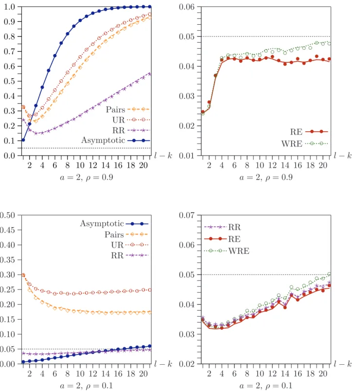
In the first two sets of experiments, the number of instruments is fairly large, with l−k = 11, and different choices for this number would have produced different results. In Figure 3, l−k varies from 1 to 21. In the top two panels, a = 2 and ρ= 0.9; in the bottom two, a = 2 andρ = 0.1. Sincea is quite small, all the tests perform relatively poorly. As before, the new bootstrap tests generally perform very much better than the older ones, although, as expected, RR is almost indistinguishable from RE when ρ= 0.1.
When ρ = 0.9, the performance of the asymptotic test and the older bootstrap tests deteriorates dramatically asl−k increases. This is not evident when ρ= 0.1, however. In contrast, the performance of the efficient bootstrap tests actually tends to improve as l−k increases. The only disturbing result is in the top right-hand panel, where the RE and WRE bootstrap tests underreject fairly severely when l =k ≤3, that is, when there are two or fewer overidentifying restrictions. The rest of our experiments do not deal with this case, and so they may not accurately reflect what happens when the number of instruments is very small.
In all the experiments discussed so far, n = 400. It makes sense to use a reasonably large number, because cross-section data sets with weak instruments are often fairly large. However, using a very large number would have greatly raised the cost of the experiments. Using larger values ofnwhile holdinga fixed would not necessarily cause any of the tests to perform better, because, in theory, rejection frequencies approach nominal levels only as both n and a tend to infinity. Nevertheless, it is of interest to see what happens as n changes while we hold a fixed.
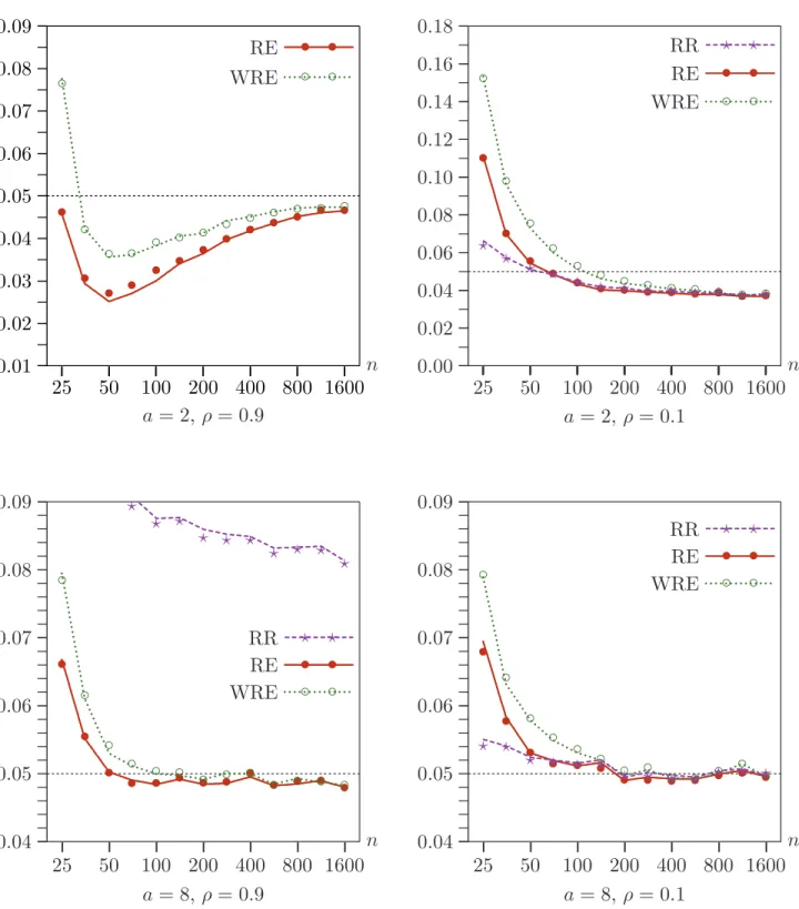
Figure 4 shows how the efficient bootstrap methods perform in four cases (a = 2 or a = 8, andρ= 0.1 orρ= 0.9) for sample sizes that increase from 25 to 1600 by factors of approximately √2. Note that, as n increases, the instruments become very weak indeed when a = 2. For n = 1600, the R2
of the reduced-form regression (28) in the DGP, evaluated at the true parameter values, is just 0.0025. Even when a = 8, it is just 0.0385.
The results in Figure 4 are striking. Both the efficient bootstrap methods perform better forn= 1600 than forn= 25, often very much better. Asnincreases from 25 to about 200, the performance of the tests often changes quite noticeably. However, their performance never changes very much as n is increased beyond 400, which is why we used that sample size in most of the experiments. When possible, the figure includes rejection frequencies for RR. Interestingly, when ρ = 0.1, it actually outperforms RE for very small sample sizes, although its performance is almost indistinguishable from that of RE for n≥70.
The overall pattern of the results in Figure 4 is in accord with the asymptotic theory laid out in Section 3. In particular, the failure of the rejection frequency of the boot-strap ttests using RE and WRE to converge to the nominal level of 0.05 as ngrows is predicted by that theory. The reason is that, under weak-instrument asymptotics, no estimate of a is consistent. Nevertheless, we see from Figure 4 that this inconsistency leads to an ERP of the bootstrap test for a = 2 and large n that is quite small. It is less than 0.004 in absolute value when ρ= 0.9 and about 0.012 when ρ= 0.1.
Up to this point, we have reported results only for equal-tail bootstrap tests, that is, ones based on the equal-tail P value (8). We believe that these are more attractive in the context of t statistics than tests based on the symmetric P value (7), because IV estimates can be severely biased when the instruments are weak. However, it is important to point out that results for symmetric bootstrap tests would have differed, in some ways substantially, from the ones reported for equal-tail tests.
Figure 5 is comparable to Figure 2. It too shows rejection frequencies as functions of ρ for n= 400 and l−k = 11, witha = 2 in the top row anda= 8 in the bottom row, but this time for symmetric bootstrap tests. Comparing the top left-hand panels of Figure 5 and Figure 2, we see that, instead of overrejecting, symmetric bootstrap tests based on the pairs and UR bootstraps underreject severely when the instruments are weak and ρ is small, although they overreject even more severely than equal-tail tests when ρ is very large. Results for the RR bootstrap are much less different, but the symmetric version underrejects a little bit more than the equal-tail version for small values of ρ and overrejects somewhat more for large values.
As one would expect, the differences between symmetric and equal-tail tests based on the new, efficient bootstrap methods are much less dramatic than the differences for the pairs and UR bootstraps. At first glance, this statement may appear to be false, because the two right-hand panels in Figure 5 look quite different from the corresponding ones in Figure 2. However, it is important to bear in mind that the vertical axes in the right-hand panels are highly magnified. The actual differences in
rejection frequencies are fairly modest. Overall, the equal-tail tests seem to perform better than the symmetric ones, and they are less sensitive to the values of ρ, which further justifies our choice to focus on them.
Next, we turn our attention to heteroskedasticity. The major advantage of the WRE over the RE bootstrap is that the former accounts for heteroskedasticity in the boot-strap DGP and the latter does not. Thus it is of considerable interest to see how the various tests (now including AR and K) perform when there is heteroskedasticity. In principle, heteroskedasticity can manifest itself in a number of ways. However, because there is only one exogenous variable that actually matters in the DGP given by (27) and (28), there are not many obvious ways to model it without using a more complicated model. In our first set of experiments, we used the DGP
y1 =n1/2|w1| ∗u1 (29)
y2 =aw1+u2, u2 =ρn1/2|w1| ∗u1+rv, (30)
where, as before, the elements ofu1 andv are independent and standard normal. The
purpose of the factor n1/2
is to rescale the instrument so that its squared length is n instead of 1. Thus each element of u1 is multiplied by the absolute value of the
corresponding element of w1, appropriately rescaled.
We investigated rejection frequencies as a function of ρ for this DGP for two values of a, namely, a = 2 and a = 8. Results for the new, efficient bootstrap methods only are reported in Figure 6. These results are comparable to those in Figure 2. There are four test statistics (ts, th, AR, and K) and two bootstrap methods (RE and WRE).
The left-hand panels contain results for a = 2, and the right-hand panels for a = 8. The top two panels show results for three tests that work badly, and the bottom two panels show results for five tests that work at least reasonably well.
The most striking result in Figure 6 is that using RE, the bootstrap method which does not allow for heteroskedasticity, along with any of the test statistics that require homoskedasticity (ts, AR, and K) often leads to severe overrejection. Of course, this
is hardly a surprise. But the result is a bit more interesting if we express it in another way. Using either WRE, the bootstrap method which allows for heteroskedasticity,or the test statistic th, which is valid in the presence of heteroskedasticity of unknown
form, generally seems to produce rejection frequencies that are reasonably close to nominal levels.
This finding can be explained by the standard result, discussed in Section 3, under which bootstrap tests are asymptotically valid whenever one of two conditions is satis-fied. The first is that the quantity is asymptotically pivotal, and the second is that the bootstrap DGP converges in an appropriate sense to the true DGP. The first condition is satisfied by th but not by ts. The second condition is satisfied by WRE but not by
RE except when the true DGP is homoskedastic.
Interestingly, the combination of the AR statistic and the WRE bootstrap works ex-tremely well. Notice that rejection frequencies for AR do not depend on ρ, because
this statistic is solely a function of y1. When a = 8, combining WRE with th also
performs exceedingly well, but this is not true when a= 2.
We also performed a second set of experiments in which the DGP was similar to (29) and (30), except that each element of u1 was multiplied by n1/2w21i instead of by
n1/2
|w1i|. Thus the heteroskedasticity was considerably more extreme. Results are
not shown, because they are qualitatively similar to those in Figure 6, with WRE continuing to perform well and RE performing very poorly (worse than in Figure 6) when applied to the statistics other than th.
The most interesting theoretical results of Section 3 deal with the asymptotic validity of the WRE bootstrap applied to AR, K, ts, and th under weak instruments and
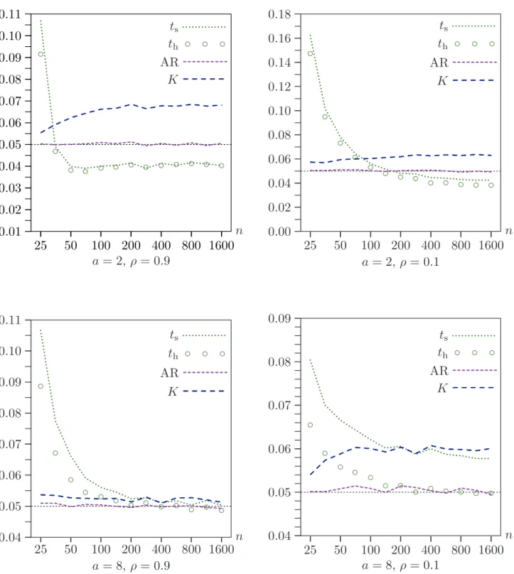
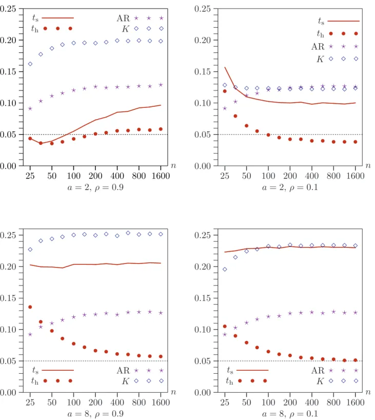
heteroskedasticity. To see whether these results provide a good guide in finite samples, we performed another set of experiments in which we varied the sample size from 25 to 1600 by factors of approximately √2 and used data generated by (29) and (30). Results for the usual four cases (a = 2 or a= 8, and ρ= 0.1 or ρ = 0.9) are shown in Figure 7. Since the AR andK tests are not directional, upper-tail bootstrap P values based on (7) were computed for them, while equal-tail bootstrap P values based on (8) were computed for the two t tests.
Figure 7 provides striking confirmation of the theory of Section 3. The AR test not only demonstrates its asymptotic validity but also performs extremely well for all sample sizes. As it did in Figure 4, th performs well for large sample sizes when a= 8, but it
underrejects modestly when a= 2. The other tests are somewhat less satisfactory. In particular, the K test performs surprising poorly in two of the four cases.
Figure 8 contains results for the RE bootstrap for the same experiments as Figure 7. All of the tests exceptthnow overreject quite severely for all sample sizes. Thus, as the
theory predicts, only th is seen to be asymptotically valid for large enough a. Careful
examination of Figures 7 and 8, which is a bit difficult because of the differences in the vertical scales, also shows that, for samples of modest size, th performs considerably
better when bootstrapped using WRE rather than RE. This makes sense, since with WRE there is the possibility of an asymptotic refinement.
Taken together, our results for both the homoskedastic and heteroskedastic cases sug-gest that the safest approach is undoubtedly to use the WRE bootstrap with the AR statistic. It is also reasonably safe to use the WRE bootstrap with the robust t statistic th when the sample size is moderate to large (say, 200 or more) and the
instruments are not extremely weak. Using the RE bootstrap, or simply performing an asymptotic test, with any statistic except th can be very seriously misleading when
heteroskedasticity is present.
5. More than Two Endogenous Variables
Up to this point, as in Davidson and MacKinnon (2008), we have focused on the case in which there is just one endogenous variable on the right-hand side. The AR test (23), the K test, and the CLR test are designed to handle only this special case. However,
there is no such restriction for tstatistics, and the RE and WRE bootstraps can easily be extended to handle more general situations.
For notational simplicity, we deal with the case in which there are just two endogenous variables on the right-hand side. It is trivial to extend the analysis to handle any number of them. The model of interest is
y1 =β2y2+β3y3+Zγ+u1 (31)
y2 =Wπ2+u2 (32)
y3 =Wπ3+u3, (33)
where the notation should be obvious. As before, Z andW are, respectively, ann×k and ann×l matrix of exogenous variables with the property that S(Z) lies in S(W).
For identification, we require that l ≥k+ 2.
The pairs and UR bootstraps require no discussion. The RR bootstrap is also quite easy to implement in this case. To test the hypothesis that, say, β2 =β20, we need to
estimate by 2SLS a restricted version of equation (31),
y1−β20y2 =β3y3+Zγ+u1, (34)
in which y3 is the only endogenous right-hand side variable, so as to yield restricted
estimates ˜β3 and ˜γ and 2SLS residuals ˜u1. We also estimate equations (32) and (33)
by OLS, as usual. Then the bootstrap DGP is yi∗1−β20y ∗ i2 = ˜β3y ∗ 3i+Ziγ˜+ ˜u∗1i y2∗i =Wiπˆ2+ ˆu ∗ 2i (35) y3∗i =Wiπˆ3+ ˆu ∗ 3i,
where the bootstrap disturbances are generated as follows: ˜ u∗ 1i ˆ u∗ 2i ˆ u∗ 3i ∼EDF ˜ u1i n/(n−l)1/2 ˆ u2i n/(n−l)1/2 ˆ u3i . (36)
As before, we may omit the term Ziγ˜ from the first of equations (35). In (36), we rescale the OLS residuals from the two reduced-form equations but not the 2SLS ones from equation (34), although this is not essential.
For the RE and WRE bootstraps, we need to re-estimate equations (32) and (33) so as to obtain more efficient estimates that are asymptotically equivalent to 3SLS. We do so by estimating the analogs of regression (15) for these two equations, which are
y2 =Wπ2+δ2u˜1+ residuals, and
We then use the OLS estimates ˜π2 and ˜π3 and the residuals ˜u2 ≡ y2 −Wπ˜2 and
˜
u3 ≡y3−Wπ˜3 in the RE and WRE bootstrap DGPs:
yi∗1−β20y ∗ i2 = ˜β3y ∗ 3i+Ziγ˜+ ˜u∗1i y2∗i =Wiπ˜2+ ˜u ∗ 2i (37) y3∗i =Wiπ˜3+ ˜u ∗ 3i.
Only the second and third equations of (37) differ from the corresponding equations of (35) for the RR bootstrap. In the case of the RE bootstrap, we resample from triples of (rescaled) residuals: ˜ u∗ 1i ˜ u∗ 2i ˜ u∗ 3i ∼EDF ˜ u1i n/(n−l)1/2 ˜ u2i n/(n−l)1/2 ˜ u3i .
In the case of the WRE bootstrap, we use the analog of (19), which is ˜ u∗ 1i ˜ u∗ 2i ˜ u∗ 3i = ˜ u1ivi∗ n/(n−l)1/2 ˜ u2ivi∗ n/(n−l)1/2 ˜ u3ivi∗ , where v∗
i is a suitable random variable with mean 0 and variance 1.
6. Bootstrap Confidence Intervals
Every confidence interval for a parameter is constructed, implicitly or explicitly, by inverting a test. We may always test whether any given parameter value is the true value. The upper and lower limits of the confidence interval are those values for which the test statistic equals its critical value. Equivalently, for an interval with nominal coverage 1−α based on a two-tailed test, they are the parameter values for which the P value of the test equals α. For an elementary exposition, see Davidson and MacKinnon (2004, Chapter 5).
There are many types of bootstrap confidence interval; Davison and Hinkley (1997) provides a good introduction. The type that is widely regarded as most suitable is the
percentile t, orbootstrap t, interval. Percentilet intervals could easily be constructed
using the pairs or UR bootstraps, for which the bootstrap DGP does not impose the null hypothesis, but they would certainly work badly whenever bootstrap tests based on these methods work badly, that is, whenever ρ is not small and a is not large; see Figures 1, 2, 3, and 5.
It is conceptually easy, although perhaps computationally demanding, to construct confidence intervals using bootstrap methods that do impose the null hypothesis. We now explain precisely how to construct such an interval with nominal coverage 1−α.
The method we propose can be used with any bootstrap DGP that imposes the null hypothesis, including the RE and WRE bootstraps. It can be expected to work well whenever the rejection frequencies for tests at levelα based on the relevant bootstrap method are in fact close to α.
1. Estimate the model (1) and (2) by 2SLS so as to obtain the IV estimate ˆβ and the heteroskedasticity-robust standard errorsh( ˆβ) defined in (6). Our simulation
results suggest that there is no significant cost to using the latter rather than the usual standard error that is not robust to heteroskedasticity, even when the disturbances are homoskedastic, for the sample sizes typically encountered with cross-section data.
2. Write a routine that, for any value of β, say β0, calculates a test statistic for the
hypothesis that β =β0 and bootstraps it under the null hypothesis. This routine
must perform B bootstrap replications using a random number generator that depends on a seed m to calculate a bootstrap P value, say p∗
(β0). For th, this
should be an equal-tail bootstrap P value based on equation (8). For the AR or K statistics, it should be an upper-tail one.
3. Choose a reasonably large value of B such that α(B + 1) is an integer, and also choose m. The same values of m and B must be used each time p∗
(β0)
is calculated. This is very important, since otherwise a given value of β0 would
yield different values of p∗
(β0) each time it was evaluated.
4. For the lower limit of the confidence interval, find two values ofβ, sayβl− andβl+,
with βl− < βl+, such that p∗(βl−) < α and p∗(βl+)> α. Since both values will
normally be less than ˆβ, one obvious way to do this is to start at the lower limit of an asymptotic confidence interval, say β∞
l , and see whether p
∗
(βl) is greater
or less than α. If it is less than α, then β∞
l can serve as βl−; if it is greater, then β∞
l can serve as βl+. Whichever of βl− and βl+ has not been found in this
way can then be obtained by moving a moderate distance, perhaps sh( ˆβ), in the
appropriate direction as many times as necessary, each time checking whether the bootstrap P value is on the desired side ofα.
5. Similarly, find two values of β, say βu− and βu+, with βu− < βu+, such that
p∗
(βu−)> α and p∗(βu+)< α.
6. Find the lower limit of the confidence interval, β∗
l. This is a value between βl− and βl+ which is such that p∗(β∗l) ∼= α. One way to find β
∗
l is to minimize the
function p∗
(β)−α2
with respect toβ in the interval [βl−, βl+] by using golden
section search; see, for instance, Press, Teukolsky, Vettering, and Flannery (2007, Section 10.2). This method is attractive because it is guaranteed to converge to a local minimum and does not require derivatives.
7. In the same way, find the upper limit of the confidence interval, β∗
u. This is a
value between βu− and βu+ which is such thatp∗(β∗u)∼=α.
When a confidence interval is constructed in this way, the limits of the interval have the property that p∗
(β∗
l) ∼= p
∗ (β∗
become exact, subject to the termination criterion for the golden search routine, if B were allowed to tend to infinity. The problem is that p∗
(β) is a step function, the value of which changes by precisely 1/B at certain points as its argument varies. This suggests thatB should be fairly large, if possible. It also rules out the many numerical techniques that, unlike golden section search, use information on derivatives.
7. An Empirical Example
The method of instrumental variables is routinely used to answer empirical questions in labor economics. In such applications, it is common to employ fairly large cross-section datasets for which the instruments are very weak. In this cross-section, we apply our methods to an empirical example of this type. It uses the same data as Card (1995). The dependent variable in the structural equation is the log of wages for young men in 1976, and the other endogenous variable is years of schooling. There are 3010 observations without missing data, which originally came from the Young Men Cohort of the National Longitudinal Survey.
Although we use Card’s data, the equation we estimate is not identical to any of the ones he estimates. We simplify the specification by omitting a large number of exogenous variables having to do with location and family characteristics, which appear to be collectively insignificant, at least in the IV regression. We also use age and age squared instead of experience and experience squared in the wage equation. As Card notes, experience is endogenous if schooling is endogenous. In some specifications, he therefore uses age and age squared as instruments. For purposes of illustrating the methods discussed in this paper, it is preferable to have just two endogenous variables in the model, and so we do not use experience as an endogenous regressor. This slightly improves the fit of the IV regression, but it also has some effect on the coefficient of interest. In addition to age and age squared, the structural equation includes a constant term and dummies for race, living in a southern state, and living in an SMSA as exogenous variables.
We use four instruments, all of which are dummy variables. The first is 1 if there is a year college in the local labor market, the second if there is either a two-year college or a four-two-year college, the third if there is a public four-two-year college, and the fourth if there is a private four-year college. The second instrument was not used by Card, although it is computed as the product of two instruments that he did use. The instruments are fairly weak, but apparently not as weak as in many of our simulations. The concentration parameter is estimated to be just 19.92, which is equivalent to a = 4.46. Of course, this is just an estimate, and a fairly noisy one. The Sargan statistic for overidentication is 7.352. This has an asymptotic P value of 0.0615 and a bootstrap P value, using the wild bootstrap for the unrestricted model, of 0.0658. Thus there is weak evidence against the overidentifying restrictions.
Our estimate of the coefficient β, which is the effect of an additional year of schooling on the log wage, is 0.1150. This is higher than some of the results reported by Card and lower than others. The standard error is either 0.0384 (assuming homoskedasticity) or
0.0389 (robust to heteroskedasticity). Thus the t statistics for the coefficient β to be zero and the corresponding asymptotic P values are:
ts = 2.999 (p= 0.0027) and th = 2.958 (p= 0.0031).
Equal-tail bootstrap P values are very similar to the asymptotic ones. Based on B = 99,999, theP value is 0.0021 for the RE bootstrap using ts, and either 0.0021 or
0.0022 for the WRE bootstrap using th. The first of these wild bootstrap P values is
based on the Rademacher distribution (21) that imposes symmetry, and the second is based on the distribution (20) that does not.
We also compute the AR statistic, which is 5.020 and has a P value of 0.00050 based on the F(4,3000) distribution. WRE bootstrap P values are 0.00045 and 0.00049 based on (21) and (20), respectively. It is of interest that the AR statistic rejects the null hypothesis even more convincingly than the bootstrap t statistics. As some of the simulation results in Davidson and MacKinnon (2008) illustrate, this can easily happen when the instruments are weak. In contrast, the P values for theK statistic, which is 7.573, are somewhat larger than the ones for the t statistics. The asymptotic P value is 0.0059, and the WRE ones are 0.0056 and 0.0060.
Up to this point, our bootstrap results merely confirm the asymptotic ones, which suggest that the coefficient of schooling is almost certainly positive. Thus they might incorrectly be taken to show that asymptotic inference is reliable in this case. In fact, it is not. Since there is a fairly low value of a and a reasonably large value of ρ (the correlation between the residuals from the structural and reduced-form equations is −0.474), our simulation results suggest that asymptotic theory should not perform very well in this case. Indeed, it does not, as becomes clear when we examine bootstrap confidence intervals.
We construct eleven different 0.95 confidence intervals for β. Two are asymptotic intervals based on ts and th, two are asymptotic intervals obtained by inverting the
AR and K statistics, and seven are bootstrap intervals. The procedure for inverting the AR and K statistics is essentially the same as the one discussed in Section 6, except that we use either the F(4,3000) orχ2
(1) distributions instead of a bootstrap distribution to compute P values. One bootstrap interval is based on ts with the RE
bootstrap. The others are based on th, AR, and K, each with two different variants
of the WRE bootstrap. The “s” variant uses (21) and thus imposes symmetry, while the “ns” variant uses (20) and thus does not impose symmetry. In order to minimize the impact of the specific random numbers that were used, all bootstrap intervals are based on B = 99,999. Each of them required the calculation of at least 46 bootstrap P values, mostly during the golden section search. Computing each bootstrap interval took about 30 minutes on a Linux machine with an Intel Core 2 Duo E6600 processor.
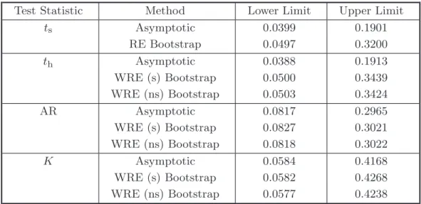
Table 1. Confidence Intervals for β
Test Statistic Method Lower Limit Upper Limit
ts Asymptotic 0.0399 0.1901 RE Bootstrap 0.0497 0.3200 th Asymptotic 0.0388 0.1913 WRE (s) Bootstrap 0.0500 0.3439 WRE (ns) Bootstrap 0.0503 0.3424 AR Asymptotic 0.0817 0.2965 WRE (s) Bootstrap 0.0827 0.3021 WRE (ns) Bootstrap 0.0818 0.3022 K Asymptotic 0.0584 0.4168 WRE (s) Bootstrap 0.0582 0.4268 WRE (ns) Bootstrap 0.0577 0.4238
It can be seen from Table 1 that, for the t statistics, the lower limits of the bootstrap intervals are moderately higher than the lower limits of the asymptotic intervals, and the upper limits are very much higher. What seems to be happening is that ˆβ is biased downwards, because ρ < 0, and the standard errors are also too small. These two effects almost offset each other when we test the hypothesis that β = 0, which is why the asymptotic and bootstrap tests yield such similar results. However, they do not fully offset each other for the tests that determine the lower limit of the confidence interval, and they reinforce each other for the tests that determine the upper limit. All the confidence intervals based on the AR statistic are substantially narrower than the bootstrap intervals based on the t statistics, although still wider than the asymp-totic intervals based on the latter. In contrast, the intervals based on the K statistic are even wider than the bootstrap intervals based on the t statistics. This is what one would expect based on theP values for the tests of β = 0. Of course, if the overidenti-fying restrictions do not hold, the AR statistic will tend to overreject. Bootstrapping does not make much difference for AR and K, apparently because there is not much heteroskedasticity.
It is perhaps a bit disappointing that the bootstrap confidence intervals in Table 1 are so wide. This is a consequence of the model and the data, not the bootstrap methods themselves. With stronger instruments, the estimates would be more precise, all the confidence intervals would be narrower, intervals based on t statistics would be narrower relative to ones based on the AR statistic, and the differences between bootstrap and asymptotic intervals based on t statistics would be less pronounced.
8. Conclusion
In this paper, we propose a new bootstrap method for models estimated by instru-mental variables. It is a wild bootstrap variant of the RE bootstrap proposed in Davidson and MacKinnon (2008). The most important features of this method are that it uses efficient estimates of the reduced-form equation(s) and that it allows for heteroskedasticity of unknown form.
We prove that, when the new WRE bootstrap is applied to the Anderson-Rubin stat-istic under weak instrument asymptotics and heteroskedasticity of unknown form, it yields an asymptotically valid test. We also show that it does not do so when it is applied to t statistics and the K statistic. Under strong instrument asymptotics, it yields asymptotically valid tests for all the test statistics.
In an extensive simulation study, we apply the WRE bootstrap and several existing bootstrap methods totstatistics, which may or may not be robust to heteroskedasticity of unknown form, for the coefficient of a single endogenous variable. We also apply the WRE bootstrap to the AR and K statistics when there is heteroskedasticity. We find that, like the RE bootstrap, the new WRE bootstrap performs very much better than earlier bootstrap methods, especially when the instruments are weak.
We also show how to apply the RE and WRE bootstraps to models with two or more endogenous variables on the right-hand side, but their performance in this context remains a topic for future research. In addition, we discuss how to construct confidence intervals by inverting bootstrap tests based on bootstrap DGPs that impose the null hypothesis, such as the RE and WRE bootstraps.
Finally, we apply the efficient bootstrap methods discussed in this paper to an empirical example that involves a fairly large sample but weak instruments. When used to test the null hypothesis that years of schooling do not affect wages, the new bootstrap tests merely confirm the results of asymptotic tests. However, when used to construct confidence intervals, they yield intervals that differ radically from conventional ones based on asymptotic theory.
References
Andrews, D. W. K., Moreira, M. J., and Stock, J. H. (2006), “Optimal Two-Sided Invariant Similar Tests for Instrumental Variables Regression,” Econometrica, 74, 715–752.
Anderson, T. W., and Rubin, H. (1949), “Estimation of the Parameters of a Single Equation in a Complete System of Stochastic Equations,” Annals of Mathematical Statistics, 20, 46–63.
Beran, R. (1988), “Prepivoting Test Statistics: A Bootstrap View of Asymptotic Refinements,” Journal of the American Statistical Association, 83, 687–697. Card, D. (1995), “Using Geographic Variation in College Proximity to Estimate the
Return to Schooling,” in Aspects of Labour Market Behaviour: Essays in Honour of J. Vanderkamp, eds. L. N. Christofides, E. K. Grant, and R. Swidinsky,
Toronto: University of Toronto Press, pp. 201–222.
Davidson, R., and Flachaire, E. (2008), “The Wild Bootstrap, Tamed at Last,” Journal of Econometrics, 146, 162–169.
Davidson, R., and MacKinnon, J. G. (1999), “The Size Distortion of Bootstrap Tests,” Econometric Theory, 15, 361–376.
Davidson, R., and MacKinnon, J. G. (2000), “Bootstrap Tests: How Many Bootstraps?,” Econometric Reviews, 19, 55–68.
Davidson, R., and MacKinnon, J. G. (2004), Econometric Theory and Methods, New York: Oxford University Press.
Davidson, R., and MacKinnon, J. G. (2008), “Bootstrap Inference in a Linear Equation Estimated by Instrumental Variables,” Econometrics Journal, 11, 443–477.
Davison, A. C., and Hinkley, D. V. (1997),Bootstrap Methods and Their Applica-tion, Cambridge: Cambridge University Press.
Dufour, J.-M., and Taamouti, M. (2005), “Projection-Based Statistical Inference in Linear Structural Models with Possibly Weak Instruments,” Econometrica, 73, 1351–1365.
Dufour, J.-M., and Taamouti, M. (2007), “Further Results on Projection-Based Inference in IV Regressions with Weak, Collinear or Missing Instruments,” Journal of Econometrics, 139, 133–153.
Flores-Lagunes, A. (2007), “Finite Sample Evidence of IV Estimators under Weak Instruments,” Journal of Applied Econometrics, 22, 677–694.
Freedman, D. A. (1981), “Bootstrapping Regression Models,” Annals of Statistics, 9, 1218–1228.
Freedman, D. A. (1984), “On Bootstrapping Two-Stage Least-Squares Estimates in Stationary Linear Models,” Annals of Statistics, 12, 827–842.
Gon¸calves, S., and Kilian, L. (2004), “Bootstrapping Autoregressions with Heteroskedasticity of Unknown Form,” Journal of Econometrics, 123, 89–120. Horowitz, J. L. (2001), “The Bootstrap,” Ch. 52 in Handbook of Econometrics
Vol. 5, eds. J. J. Heckman and E. E. Leamer, Amsterdam: North-Holland, 3159–3228.
Kleibergen, F. (2002), “Pivotal Statistics for Testing Structural Parameters in Instrumental Variables Regression,” Econometrica, 70, 1781–1803.
MacKinnon, J. G. (2006), “Bootstrap methods in econometrics,” Economic Record, 82, S2-S18.
Moreira, M. J. (2003), “A Conditional Likelihood Ratio Test for Structural Models,”
Econometrica, 71, 1027–1048.
Moreira, M. J., Porter, J. R., and Suarez, G. A. (2005), “Bootstrap and Higher-Order Expansion Validity when Instruments May Be Weak,” NBER Working Paper No. 302, revised.
Press, W. H., Teukolsky, S. A., Vetterling, W. T., and Flannery, B. P. (2007),
Numerical Recipes: The Art of Scientific Computing, Third Edition, Cambridge: Cambridge University Press.
Staiger, D., and Stock, J. H. (1997), “Instrumental Variables Regression with Weak Instruments,” Econometrica, 65, 557–586.
Wu, C. F. J. (1986), “Jackknife, Bootstrap and Other Resampling Methods in Regression Analysis,” Annals of Statistics, 14, 1261–1295.