Multiscale and multiphysics computational models of processes
in shock wave lithotripsy
Daniel Fovargue
A dissertation submitted to the faculty of the University of North Carolina at Chapel Hill in partial fulfillment of the requirements for the degree of Doctor of Philosophy in the Department of Mathematics.
Chapel Hill 2013
Approved by
Sorin Mitran .
John Dolbow
Richard McLaughlin
Laura Miller
Abstract
DANIEL FOVARGUE: Multiscale and multiphysics computational models of processes in shock wave lithotripsy
(Under the direction of Sorin Mitran)
This thesis presents two computational models applied to processes in shock wave
lithotripsy. The first is a multiphysics model of the focusing of an acoustic pulse and the
subsequent shock wave formation that occurs in a refracting electromagnetic lithotripter.
This model solves both the linear elasticity equations and the Euler equations with a Tait
equation of state in arbitrary subsets of the full computational domain. It is implemented
within BEARCLAW and uses a finite-volume Riemann solver approach. The model is
validated using a standard lens design and is shown to accurately predict the effects of a
lens modification. This model is also extended to include a kidney stone simulant in the
domain in which a simple isotropic damage law is included. The second computational
model is a 3D multiscale fracture model which predicts crack formation and propagation
within a kidney stone simulant by utilizing a continuum-mesoscopic interaction. The
simulant included in the model is realistic in that the data representing the stone is
drawn from µCT image data. At the continuum scale the linear elasticity equations are
solved while incorporating an anisotropic damage variable, again using a finite-volume
Riemann solver within BEARCLAW. At the mesoscale, damage accumulates based on
experimentally informed probability distributions and on predefined surfaces representing
are discussed. These include probability distributions of fracture properties found from
ACKNOWLEDGMENTS
I first and most of all want to thank my wife and best friend, Lauren, for her continual
support. My most valuable experience in graduate school was meeting her.
I would like to thank my advisor, Sorin Mitran, for his guidance and teaching. His
explanations of mathematical and scientific concepts are unrivaled and my understanding
is much broader and deeper as a result. I also very much appreciate his commitment
to my success. I also want to thank my current and former committee members, John
Dolbow, Richard McLaughlin, Laura Miller, Pei Zhong, and Michael Minion, for their
time and effort.
I appreciate getting to work with Pei Zhong’s lithotripsy group at Duke and would
like to especially thank Jaclyn Lautz, Georgy Sankin, and Nathan Smith for their direct
contributions to this work and their help along the way. I would also like to thank the
members of Sorin Mitran’s research group, Greg Herschlag, Anil Shenoy, Paula Vasquez,
Christoph Kirsch, and Jennifer Young.
Thank you to the friends and officemates at UNC who helped make my time at
graduate school the great experience it was, especially Emily Braley, Matthew Christian,
J.D. Martindale, and Brandyn Lee, although there are many others too. Thank you as
well to the many other professors, staff members, and students who make the UNC math
I would like to thank Grady Lemoine and Randy LeVeque for taking time to offer
some help. Also, thank you to the Biomedical Research Imaging Center, especially Kevin
Guley and Brandon Frederick, for the MicroCT imaging.
Thank you to all the amazing professors and teachers I’ve been lucky to have during
all of my education. Finally, thank you to my parents, Kathy and Art, and my sister,
Rachel, for their love and support, without which I couldn’t have gotten this far.
Table of Contents
List of Tables . . . viii
List of Figures . . . ix
Chapter 1. Introduction . . . 1
1.1. State of the Art . . . 3
2. Background . . . 11
2.1. Shock Wave Lithotripsy . . . 11
2.2. Continuum Damage Mechanics . . . 16
2.3. Fracture Mechanics . . . 20
3. Finite-Volume Riemann-Solvers . . . 26
3.1. Analytical Considerations . . . 27
3.2. Numerical Implementation . . . 30
3.3. Elasticity Equations . . . 39
3.4. Euler Equations . . . 55
3.5. Modifications to Current Implementations . . . 61
3.6. Verification of Method . . . 65
4. Experimental Methods . . . 69
4.1. Experimental Data Acquisition - Focusing Model . . . 69
4.2. Experimental Data Acquisition - Fracture Model . . . 73
4.3. Results . . . 85
5. Multiphysics Focusing Model . . . 95
5.1. Multiphysics . . . 97
5.2. Description of Simulation . . . 101
5.3. Results . . . 111
5.4. Discussion . . . 120
6. Multiscale Fracture Model . . . 123
6.1. Continuum Model . . . 124
6.2. Mesoscale Model . . . 136
6.3. Multiscale Interaction . . . 139
6.4. Results . . . 142
6.5. Discussion . . . 154
7. Conclusion . . . 159
8. Appendix . . . 161
8.1. Image Processing Procedure Code for Fracture Analysis 1 . . . 161
8.2. Image Processing Procedure Code for Fracture Analysis 2 . . . 167
List of Tables
Table 3.1. List of second order methods and slope limiters and their defining function. . . 34
Table 4.1. Experimentally found material properties of a 15:3 powder-to-water ratio BegoStone simulant [35]. . . 73 Table 4.2. Number of shocks required for initial fracture of a 7 mm cylindrical BegoStone kidney stone simulant over several input energies. Number of shock data for both water and butanediol is found from power fits of experimental data. . . 76
Table 4.3. The number of shocks each stone was subjected to for each µCT imaging. Bold text denotes image sets that contain clearly visible cracks. . . 78
Table 5.1. Material properties used in the 2D axisymmetric elasticity equations for water, lens (polystyrene), and stone (Ultracal-30). . . 104
Table 5.2. Comparison of lithotripter parameters calculated from experimental and numerical pressure profiles at the focus for the original lens design. Energy subscripts +1, −1, and +2 refer to the first compressive, first tensile, and second compressive wave, respectively. Rh = 6 mm was used for all pulse energy calculations.
SV is source voltage and BW is beam width. . . 116
Table 5.3. Comparison of lithotripter parameters calculated from experimental and numerical pressure profiles at the focus for the new lens design. Energy subscripts +1, −1, and +2 refer to the first compressive, first tensile, and second compressive wave, respectively. Rh = 6 mm was used for all pulse energy calculations. SV is
source voltage and BW is beam width. . . 120
List of Figures
2.1. Illustration showing the three focusing methods used in lithotripsy: reflector, lens, and spherical actuator. Electromagnetic lithotripters are not restricted to refraction and have been used with parabolic reflectors and spherical actuators. . . 13
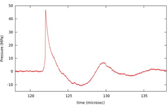
2.2. Plot of pressure over time at the focus of an electromagnetic lithotripter. (Data was recorded by Nathan Smith at Duke University using an optical hydrophone) . . . 14
2.3. Stress strain diagram for a brittle material. . . 22
3.1. Reference diagram showing a finite volume grid in 2D with labeled cells and boundaries. Also shown is an illustration of the normal and transverse fluxes resulting from the normal Riemann solve at boundary (i−1/2, j). . 35
3.2. Plots of analytically and numerically computed reflection and transmission coefficients for an acoustic pulse encountering an oblique material interface. Red corresponds to transmission coefficients and blue corresponds to reflection coefficients. Points are numerical results and lines are plots of the analytic equations. (A) Coefficients versus impedance ratios for a flat boundary, θ = 0. (B) Coefficients versus impedance ratios for an oblique boundary,θ = 0.28 radians. (C) Coefficients versus angles for z2/z1 = 1/3. (D) Coefficients versus angles for z2/z1 = 3/1. . . 67
3.3. Convergence plot of the 3D elasticity solver implemented in a finite volume Riemann solver context in BEARCLAW. . . 68
4.1. Diagram of the experimental setup with the tank, actuator, and lens in the center. Red arrows show the FOPH setup and blue arrows show the flow of water to fill the space behind the lens. Also shown is the 3-D positioning system used to position the fiber optic probe hydrophone for pressure measurement. . . 70
4.2. Plot showing the number of shocks required for initial fracture of a 7 mm cylidrical 15:3 BegoStone kidney stone simulant versus the peak positive pressure of the shock. Results for both water and butanediol as the transmission medium are included. Power fits for both sets of data are also shown. (Results recorded and plot constructed by Jaclyn Lautz) . . . . 75
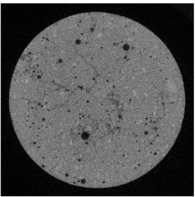
4.4. An example MicroCT image slice of a 7 mm cylindrical stone in which cracks are visible. . . 80
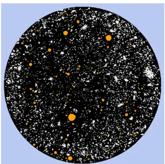
4.5. An example MicroCT image showing the four regions that the image is divided into for the crack enhancing procedure. Blue is outside the stone, gray is the lighter pixels, orange is the dark pixels, and black is the remainder which will contain the cracks. . . 81
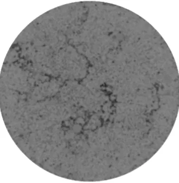
4.6. An example MicroCT image slice after being subjected to the crack enhancing image processing algorithm. . . 82
4.7. An example MicroCT image with edges shown in white from MATLAB’s
edge detection algorithm. The background is a darkened version of the crack enhanced image to help highlight the edges. . . 83
4.8. An example MicroCT image with line segments representative of cracks shown in green. The background is the crack enhanced image. . . 84
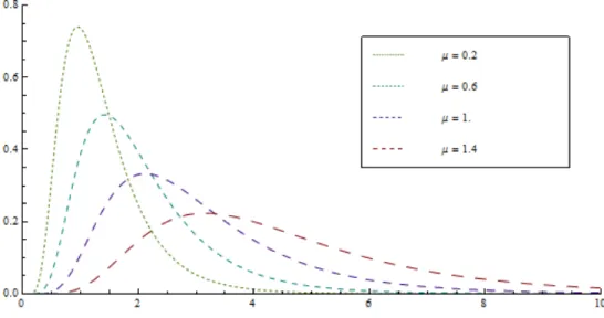
4.9. Lognormal probability distribution function for various values of µ with
φ= 0.5. . . 86
4.10. Lognormal probability distribution function for various values of φ with
µ= 1.0. . . 86
4.11. Crack length (A) and width (B) data from 7 mm cylindrical stone 1 at shock 10 meant as an example to show the lognormal fit close up. . . 87
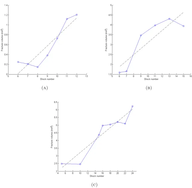
4.12. Volume of fracture calculated by automated procedure for each image set with a linear fit. (A) 7 mm cylindrical stone 1. (B) 7 mm cylindrical stone 2. (C) 10 mm cylindrical stone 1. . . 88
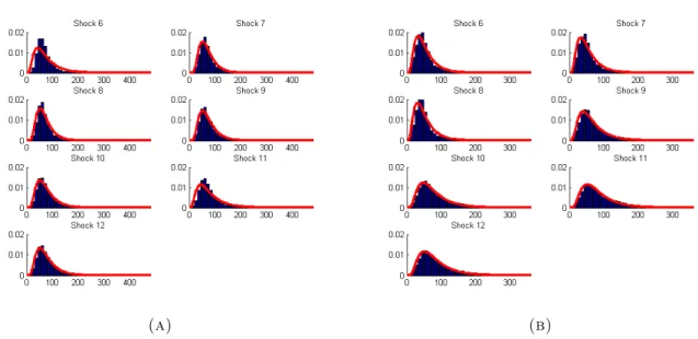
4.13. Normalized crack length and width data from 7 mm cylindrical stone 1 plotted as histograms for each shock number image set and compared to lognormal distributions. Length and width is measured inµm. Length data is shifted 24 µm left and width data is shifted 4 µm left. (A) Length. (B) Width. . . 89
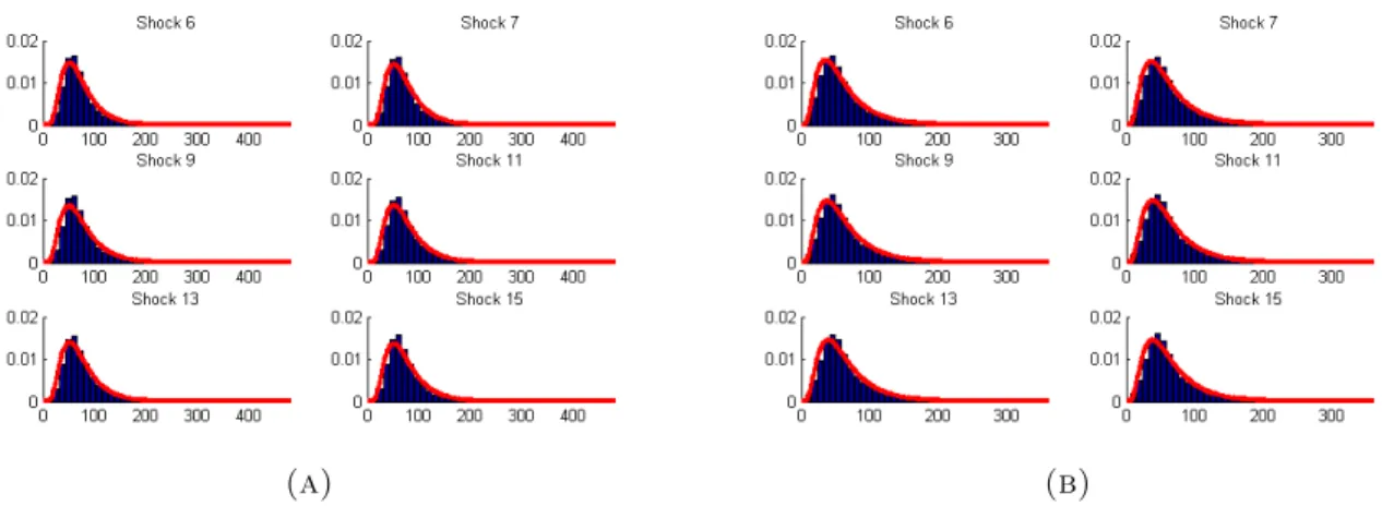
4.14. Normalized crack length and width data from 7 mm cylindrical stone 2 plotted as histograms for each shock number image set and compared to lognormal distributions. Length and width is measured inµm. Length data is shifted 24 µm left and width data is shifted 4 µm left. (A) Length. (B) Width. . . 90
4.16. Calculated parameters of the lognormal fits of the crack length and width data for each stone and shock number. (A) 7 mm cylindrical stone 1. (B) 7 mm cylindrical stone 2. (C) 10 mm cylindrical stone 1. . . 92
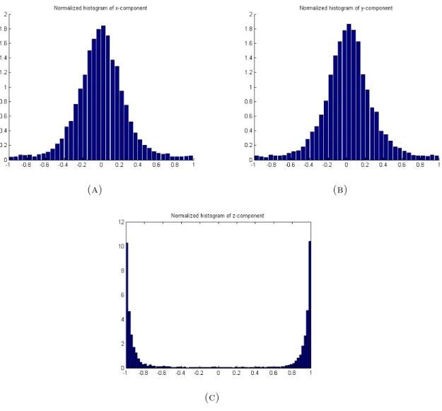
4.17. Distributions of the x (A), y (B), and z (C) components of the crack orientations vectors. . . 93
5.1. Diagram showing the domain of the focusing model when not including a kidney stone simulant. The z axis is the axis of symmetry. The incoming pulse enters along the left boundary. The geometric focus of the acoustic lens is labeled. . . 96
5.2. Reference diagram showing finite volume cells divided into Euler water, elastic water, and elastic solid regions. . . 98
5.3. Diagram showing the domain of the focusing model when using the general multiphysics implementation. The proximal surface of the stone is located at the geometric focus of the lens. The thickness of the elasticity water region is exaggerated to aid in viewing. . . 99
5.4. (A) Photograph of the two lenses used. On the left is a standard lens design. On the right is the new lens modified by an annular ring cut. (B) Diagrams of the cross sections of the two lenses, original on the left and modified on the right. r = 0 corresponds to the central axis of the lenses. . . 104
5.5. Progression of the computational solution at selected times. On the left the focusing and shock wave formation over the entire computational domain is shown. On the right the interaction of the shock wave in the fluid region and elastic stone is shown. The original lens and 15.8 kV input is used here. Within the elastic regions the average of the normal stresses is displayed as pressure. . . 109
5.6. Example comparison of the experimentally recorded hydrophone data and the numerically recorded data at the geometric focus of the lens. . . 110
5.7. Example plot of maximum pressure readings near the focus with contour lines. . . 110
5.8. Example plots of the incoming pulse for the three voltage levels predominantly used here. (A) Pressure distribution in the radial direction att= 3 µs. (B) Pressure over time atr = 40 mm. . . 113
5.10. Plots of peak positive and peak negative pressure in the focal plane (z = 181.8 mm) for the original lens. Experimental data is recorded in four directions from the z-axis (x+, x−, y+, y−). Numerical data is mirrored across r = 0 to aid in visualization. (A) 13.8 kV. (B) 15.8 kV. . . 115
5.11. Comparison of peak positive pressure (P+), peak negative pressure (P−),
and beam width for the original lens over the dynamic range of the lithotripter. Polynomial fits are also shown (dotted for experiment and solid for numerical). . . 116
5.12. Plots of experimental and numerical pressure profiles along the propagation axis, r = 0, and in the focal plane, z = 181.8 mm for the new lens. (A) Propagation axis with 15.8 kV input. (B) Propagation axis with 16.8 kV input. (C) Focal plane with 15.8 kV input. (D) Focal plane with 16.8 kV input. . . 118
5.13. Plots of peak positive and peak negative pressure in the focal plane (z = 181.8 mm) for the new lens. Experimental data is recorded in four directions from thez-axis (x+, x−, y+, y−). Numerical data is mirrored acrossr= 0 to aid in visualization. (A) 15.8 kV. (B) 16.8 kV. . . 119
5.14. Comparison of peak positive pressure (P+), peak negative pressure (P−),
and beam width for the new lens with available experimental data over the dynamic range of the lithotripter. Polynomial fits are also shown (dotted for experiment and solid for numerical) . . . 119
5.15. Comparison of the maximum over time of the maximum principal stress (A) and the damage (B) in a cylindrical kidney stone simulant with height 7 mm and radius 3 mm for the original lens with 13.8 kV input versus the new lens with 16.8 kV input after the pulse has passed completely through. 121
6.1. Diagrams of the fracture model domain. All values are in millimeters. The stone shown here corresponds to the 7 mm cylindrical stone 1 from the experimental results. (A) A slice of the 3D domain, at z = 0. (B) A contour of the edge of the stone within the full domain. . . 126
6.2. A single slice of a kidney stone simulant from both the µCT images (A) and the representation of the stone in the computational model (B). The stone shown is the 7 mm cylindrical stone 1. . . 134
6.3. Example output from Neper software. Both subfigures show the same
instance. (A) The entire cube. (B) Grains with center above 0.5 are not shown in order to view inner grains. . . 138
6.5. Time series of one shock encountering a stone in the multiscale computational fracture model. Maximum principal stress is displayed on a slice of the 3D domain. The stone is the 7 mm cylindrical stone 1 and the shock is from 18 kV input. In thet = 5.75µs frame the high tensile stress near one third the distance from the distal end of the stone is apparent. . . 143
6.6. Maximum principal stress distributions in realistic stones with no damage or fracture growth law. (A) 10 mm cylindrical stone. (B) 10 mm spherical stone. (C) 7 mm cylindrical stone 1. (D) 7 mm cylindrical stone 2. . . 145
6.7. Potential locations and directions of cracks resulting from high maximum principal stress. (A) 10 mm cylindrical stone. (B) 10 mm spherical stone. (C) 7 mm cylindrical stone 1. (D) 7 mm cylindrical stone 2. . . 146
6.8. The state of the 7 mm cylindrical stone 1 with 18 kV shock input after shocks 1 through 5. The images on the left show a 3D contour of the stone-water boundary and flat circular glyphs denote ruptured cells. The glyphs are oriented in the direction of the rupture. The images on the right show the damage in the x direction along a slice at z = 0. Water cells are colored blue and ruptured cells are colored red. . . 147
6.9. A 7 mm cylindrical BegoStone kidney stone simulant after initial fracture. Fracture reliably occurs in this stone geometry perpendicular to the propagation axis and approximately a third of the distance from the distal end of the stone. (Image by Jaclyn Lautz) . . . 148
6.10. Final stone states of 7 mm cylindrical stone 1. (A) Glyphs and 3D contour for 16 kV and 8 shocks. (B) Damage inxdirection and rupture on slices for 16 kV and 8 shocks. (C) Glyphs and 3D contour for 18 kV and 5 shocks. (D) Damage inx direction and rupture on slices for 18 kV and 5 shocks. . 149
6.11. Final stone states of 7 mm cylindrical stone 2. (A) Glyphs and 3D contour for 16 kV and 9 shocks. (B) Damage inxdirection and rupture on slices for 16 kV and 9 shocks. (C) Glyphs and 3D contour for 18 kV and 6 shocks. (D) Damage inx direction and rupture on slices for 18 kV and 6 shocks. . 150
6.12. Final stone states of the 10 mm cylindrical stone. (A) Glyphs and 3D contour for 18 kV and 5 shocks. (B) Damage in x direction and rupture on slices for 18 kV and 5 shocks. . . 151
6.13. Final stone states of the 10 mm spherical stone. (A) Glyphs and 3D contour for 18 kV and 9 shocks. (B) Damage in x direction and rupture on slices for 18 kV and 9 shocks. . . 151
6.15. Orthogonal slice of µCT image data for the 10 mm spherical stone. (A) Original image. (B) Crack covered in red to aid in viewing. . . 153
6.16. Orthogonal slice of µCT image data for 7 mm cylindrical stone 1. (A) Original image. (B) Crack covered in red to aid in viewing. . . 153
6.17. Orthogonal slice of µCT image data for 7 mm cylindrical stone 2. (A) Original image. (B) Crack covered in red to aid in viewing. . . 154 6.18. Fracture state for the 8 mm spherical struvite approximation after 5 shocks
at 18 kV. (A) Glyphs and 3D contour. (B) Damage in x direction and rupture on slices. . . 154
6.19. Fracture state for the 8 mm spherical COM approximation after 6 shocks at 18 kV. (A) Glyphs and 3D contour. (B) Damage inx-direction and rupture on slices. (C) Damage in y-direction and rupture on slices. (D) Damage in
CHAPTER 1
Introduction
This thesis presents two computational models applied to extracorporeal shock wave
lithotripsy (ESWL). ESWL is a common medical procedure used to break up kidney
stones into small enough pieces for a patient to pass naturally. In an ESWL procedure, a
strong acoustic pulse is generated outside the patient’s body and is then focused towards
the kidney stone. Depending on the type of lithotripter, the pulse begins as a shock
wave or forms into one during transit due to nonlinear steepening effects. The strong
compressive shock wave and trailing tensile wave that arrive at the stone cause damage
to it through a variety of mechanisms. This process is repeated and eventually the stone
will crack and break down into small pieces.
Both computational models use a finite-volume Riemann solver approach to
numer-ically solve the partial differential equations (PDEs) chosen to model the physics. This
method is implemented within the BEARCLAW software developed by Mitran [86] and
based on the wave propagation algorithm of LeVeque [69]. Several modifications to the
currently implemented method are also discussed in this thesis.
The first computational model is a 2D axisymmetric multiphysics simulation of
acous-tic pulse focusing and shock wave formation. An electromagneacous-tic lithotripter, which uses
a polystyrene acoustic lens for focusing, is simulated by this model. The simulation solves
domain. The linear elasticity equations are used to model the refraction of the pulse
within the lens and also the interaction of the pulse and kidney stone simulant, if a stone
is included in the model. The Euler equations with a Tait equation of state are used to
model the shock wave formation as the pulse transits from the lens towards the stone.
This model is validated by comparing to experimental results with a standard lens
de-sign. The model is then shown to accurately predicts the effects of a lens modification.
While both computational models presented in this work are applied to ESWL, they
are developed in a general way in order to make them applicable to other application
domains in potential future work.
The second computational model is a 3D multiscale simulation of fracture and damage
within a kidney stone simulant. At the larger continuum scale, the heterogeneous linear
elasticity equations are solved to model the p-wave and s-wave propagation through the
stone as the shock wave hits. The shock wave input is taken directly from the multiphysics
focusing model. The elasticity equations are extended to include an anisotropic damage
variable to inform this scale of unresolved damage and fracture. The stone geometry in
the computation is taken from µCT images of kidney stone simulants, so that realistic
stone simulants are modeled.
At a smaller mesoscale, damage accumulates on predefined surfaces within each
con-tinuum cell, typically resembling a granular structure. The amount of damage is based on
probability distributions found from experimental results. The continuum damage
vari-ables are updated according to the mesoscopic damage. Macroscopic fracture is modeled
by allowing continuum cells to rupture based on the current stress and damage state.
to experimental results. In addition, the mesoscopic structure is modified to simulate the
mesoscopic structure of certain types of real kidney stones.
Experiments in which a stone was repeatedly shocked and imaged were also conducted
as part of this work. Microscopic computed tomography, written as MicroCT or µCT,
imaging was used, which reveals the internal structure of the stone. This process was
applied to four stones and each resulted in several image sets of fracture within the stones.
A 2D image processing procedure is presented which compiles probability distributions
of crack lengths and widths. The volume of fracture and changes in these distributions
as more shocks are applied are also analyzed.
The remainder of this introduction chapter is left for a description of some of the
previously published work on topics presented in this thesis and contrasting that work
with what is presented here. In Chapter 2, background on the application domain of
ESWL is provided along with background information on continuum damage mechanics
and fracture mechanics. In Chapter 3, finite-volume Riemann solver methods are
de-scribed. Chapter 4 describes all the experimental methods used in this work and shows
some purely experimental results. Chapter 5 contains a description of the multiphysics
focusing model and results. Chapter 6 contains a description of the multiscale fracture
model and corresponding results. Finally, a conclusion is provided in Chapter 7.
1.1. State of the Art
1.1.1. Computational Models of ESWL. Several studies exist on numerical
mod-els of focusing and shock wave formation during lithotripsy. Despite the prevalence of
electromagnetic (EM) lithotipters, most works simulate focusing in either electrohydaulic
done in this thesis. Coleman et al. solved the one dimensional
Khokhlov-Zabolotskaya-Kuznetsov (KZK) equation, similar to Burgers’ equation, with the HM3 geometry [23].
Hamilton developed a linear focusing solution on the axis of symmetry of a concave
ellip-soidal mirror following the production of a spherical wave at the focus [45]. This model
was later used by Sankin et al. to investigate optical breakdown as a shock wave
gen-eration mechanism [110]. Christopher developed a nonlinear acoustic model accounting
for diffraction and attenuation and applied it to the HM3 [21, 20]. This model also
solved Burgers’ equation to account for nonlinear effects. Steiger [117] presented a finite
difference model of a reflecting EM lithotripter and accounted for attenuation in tissue.
Averkiou and Cleveland solved the 2D KZK equation to model an EH lithotripter [8].
Zhou and Zhong expanded on this model to investigate reflector geometry modifications
[137]. Ginter et. al. [40] modeled a reflecting EM lithotripter by solving nonlinear
acoustic equations by a 2D FDTD method.
Tanguay [120], in his disertation work, used a WENO method to solve the Euler
equations for two phase flow in order to investigate the bubble cloud that forms due to the
shock wave. Krimmel, Colonius, and Tanguay [61] expanded on this model to investigate
the effect of bubbles on the focusing and shock wave formation in both ellipsoid reflector
and spherical actuator. This work also incorporated the effect of tissue surrounding the
stone. Iloreta [50] investigated possible inserts into an ellipsoidal reflector lithotripter
and their effect on cavitation potential. CLAWPACK [69] was used in this work to solve
the Euler equations.
The focusing model presented here is similar to recent work but incorporates a
mul-tiphysics aspect which allows it to model acoustic wave propagation in both solids and
lithotripters which are a common type of lithotripter, and not previously modeled. This
model will potentially aid in the design of new lenses for refracting electromagnetic
lithotripters, and due to the relative ease of replacing lenses in these lithotripters, this is
a promising route to improving the procedure. This model also allows for straightforward
inclusion of additional linear elastic solids other than the lens. If there is future interest
in including stone holders, add-ons to lenses, or other objects this model can be easily
adapted.
Some models of fracture or stress distributions within kidney stones or kidney stone
simulants have also been developed. Dahake and Gracewski [27, 28] used a finite
dif-ference scheme to analyze strain within circular and cylindrical stones and compared to
experiment. They found locations of high strains due to focusing off of the distal surfaces
of the stones. Lokhandwalla and Sturtevant [77] used a spring model to approximate the
number of shocks required for the initial fracture of a kidney stone. Mihradi et. al. [82]
used a finite element method to investigate stresses within stones. The authors looked
at a variety of input pulses and also included a fracture model which compared well with
experiments.
Works by Cleveland and Sapozhnikov [22] and Sapozhnikov et. al. [111] solved
the axisymmetric elasticity equations using a centered finite difference scheme which
modeled stones surrounded by fluid. The location of the greatest maximum principal
stress over time was recorded and compared to the location of the initial fracture in an
experimental setup. Several different configurations involving a cylindrical stone were
tested. Wijerathne et. al. [128] applied a 3D dynamic fracture model called PDS-FEM
to this problem and were able to predict the initial fracture of one stone configuration.
stones taken from µCT imaging, and investigated stress distributions within. Similar to
previous work on simulants, the conclusion was that strong shear waves created when a
shock wave with large focal width hits the stone lead to high tensile stresses within the
stone.
The fracture model presented in this work differs in several key ways from previous
work. First, this work uses both realistic stone geometries taken from µCT images and
realistic shock waves taken directly from the focusing model. Incorporation of more real
world aspects should lend validity and accuracy to the model. In contrast to previous
work, this work investigates the total number of shocks required for initial fracture of
stones. This is accomplished by using a damage variable to model unresolved damage
and fracture. Stone simulants rarely fracture after one shock and in many cases fracture
after a repeatable number of shocks with very little variance. In previous work, if a
shock passes through the stone without causing fracture, there will be no difference in
the stone. Mihradi et. al. [82] and Wijerathne et. al. [128] do use the Tuler-Butcher
criterion [123] which is based on accumulation of damage. However, tracking of damage
itself and its effect on subsequent shocks is not included. These works also only investigate
single shocks. The damage model in this work is informed by statistics collected from
experiment while previous work is deterministic. Finally, this work includes mesoscopic
structures able to simulate granular or other realistic mesostructures of simulants or real
kidney stones.
1.1.2. µCT Imaging of Fracture. µCT imaging has been used successfully to image
rocks and other brittle materials similar to the kidney stone simulants in this work [130].
Some examples of usingµCT imaging to aid in fracture analysis of brittle materials before
and after loading include work by Landiset. al. [62, 63] and Renardet. al. [105]. Other
work involving imaging of brittle fracture includes [3, 24, 58, 108, 124, 125]. Although
not directly relevant to this thesis, a few selected works on imaging of metals and ductile
fracture include [6, 9, 79, 88, 122].
1.1.3. Computational Fracture. The two main goals of computational fracture
me-chanics are to solve for the distribution of stresses near a crack and to predict growth of
a crack. Some computational fracture methods will now be discussed. This list is not
meant to be exhaustive, but is presented as a sampling of existing methods.
The most widely used method in computational fracture is the finite element method
(FEM) [4]. This method lends itself well to this problem because it is straightforward
within the confines of the method to model the complicated geometry of existing cracks
and to produce a finer mesh near crack tips. This can be done with finite difference and
finite volume methods but these require extra implementation features to explicitly
rep-resent the crack and therefore aren’t as well suited for modeling complicated geometries
[90]. Remeshing is one drawback of FEM that comes about when modeling crack growth
and propagation. Since typically a finer mesh is required near the crack tip than further
away from it, the geometry is meshed in that way, but when the crack propagates a new
mesh must be developed to correspond to the new location of the crack tip. This is
es-pecially difficult when modeling nonlinear materials where a stress history is important.
Alternatively, the mesh can be refined where the crack is expected to propagate [4].
In an FEM implementation, fracture parameters can be computed using various
to compute stress intensity factors [57]. TheJ integral can be computed through
numer-ical integration [17]. The virtual crack extension method calculates the energy release
rate [46, 95]. A more efficient and versatile approach developed more recently called the
energy domain integral method also calculates the J integral [113]. When computing
crack propagation a fracture criterion must be used and when this is met finite elements
are either removed or separated.
Several methods exist which employ the FEM framework but do not require the
finite elements to explicitly represent the crack. The eXtended Finite Element Method
(X-FEM), developed by Belytschko, Black, Mo¨es, and Dolbow in a series of works [11,
31, 87], allows for fracture modeling in a FEM implementation in which the cracks are
independent of the finite element mesh. This is done by enriching the element nodes
near cracks by a discontinuous function. A similar method called E-FEM, developed by
Oliver [91, 92, 93], enriches the elements instead of the nodes. PDS-FEM, developed
by Hori, Oguni, Sakaguchi, and Wijerathne [48, 129], as mentioned above, was applied
to the problem of kidney stone fragmentation. Like the other methods, PDS-FEM uses
functions with discontinuities to represent the effect of cracks. Meshless methods, such as
the element-free Galerkin method [12], which discretize the domain with an unstructured
set of nodes, have also been used to model fracture [13].
The previous methods solve continuum equations informed in some way of a crack
discontinuity. Another set of methods model fracture by simulating a set of interacting
objects, such as a mass-spring system, and are generally called lattice models. These are
typically used for mesoscale simulations of materials and have been successfully applied to
brittle fracture. An example would be a simulation of granular fracture in concrete, where
linear elasticity. Lattice methods were first described in 1941 by Hrennikoff [49]. They
have been developed with both beam theory [30, 47, 72, 112] and with spring systems
[14, 26, 53, 56].
Fracture has also been modeled with atomistic models. These models are very
ac-curate due to the incorporation of the true small scale physics that leads to fracture.
However, they are unable to model large scale fracture simply due to the vast number of
atoms required. Even on the most powerful computers they are restricted to very small
spatial and temporal domains. Some work on fracture using these methods includes
[29, 38, 39, 44, 54].
1.1.4. Multiscale Fracture. Multiscale computations of fracture are an attractive
op-tion since they can theoretically achieve the accuracy of atomistic type methods over
larger spatial and longer time scales. This is typically accomplished by only computing
on the small scale when and where necessary and solving continuum equations away from
cracks and defects.
Kohlhoff et. al. [59] proposed a finite element combined with atomistic (FEAt)
model. This method joined a lattice atomistic model with a continuum finite element
model by a transition region which used displacements to link the two regions. The
original work applied the method to crack propagation in bcc crystals and later work by
Gumbsch and Beltz [43] applied it to additional fracture problems. Tadmor, Ortiz, and
Phillips [119] developed the Quasicontinuum (QC) method which also employs finite
element and atomistic models. Here, the domain is discretized by finite elements and
are based on atomistic calculations. This method has been successfully applied to fracture
as well [84, 85].
The coupling length scales (CLS) [2, 16, 109] and finite element, molecular dynamics,
tight-binding (FE MD TB) methods [1] use a similar transition region as the FEAt model
to connect finite element and atomistic regions, but employ a linear elastic approximation.
The coupled atomistic and discrete dislocation (CADD) [114] method also employs a
transition zone but includes a continuum representation of defects and discontinuities
which allows for larger models of plastic flow [25]. The bridging scale decomposition
method [127] relates MD and continuum mechanics by projecting the MD solution onto
the coarse scale basis functions. Details of the above mentioned methods, as well as
additional methods and comparisons between methods can be found in review papers
such as [25, 85, 94].
The work presented here models fracture at the continuum level but informed by
mesoscopic structures. In most multiscale fracture simulations, the model attempts to
capture the true molecular physics leading to fracture, whereas in this work that level
remains unresolved. Therefore, for this work, the multiscale model is described as being
a continuum-mesoscopic interaction. This work also uses a finite volume implementation
compared to most work that uses finite elements. The finite volume implementation is
retained in order for the model to work seamlessly with the focusing model as well as
CHAPTER 2
Background
This chapter contains a discussion on background material associated with this work.
The first section describes the application domain of this project, which is shock wave
lithotripsy. Next, background is provided on the solid mechanics aspects of the work,
which includes a discussion on continuum damage mechanics and fracture mechanics.
2.1. Shock Wave Lithotripsy
During the 1990s 70–80% of kidney stones were treated using ESWL, with
uretero-scopic stone removal and percutaneous nephrolithotomy accounting for the remainder
[75]. The latter is a surgical technique reserved for large stones. One main and constant
advantage of ESWL over the other two techniques is a lower complication rate and a
shorter hospital stay. Recent technological advances have increased the efficacy of the
ureteroscopic stone removal techniques, but ESWL remains the first treatment choice for
most stones of size less than 2.5 cm [75].
ESWL was developed in 1980 [19] and first introduced clinically in 1984 with the
Dornier HM3 lithotripter [73, 74]. This lithotripter was proven to be very effective and
has stone-free rates, meaning the procedure was successful, of 77-90%. The disadvantages
of this lithotripter, including the size, water bath, and the amount of anesthesia required
caused many new lithotripters to be designed. Most of these machines are less effective,
Only recently have modern lithotripters approached the stone-free rates of the Dornier
HM3 [83].
There are three types of pulse generation used in lithotripters. These are
electro-hydraulic (EH), piezoelectric (PE), and electromagnetic (EM). The Dornier HM3 is an
example of an EH lithotripter. This type uses an ellipsoid reflector and a spark discharge
at one focus of the ellipsoid to create a shock wave. The shock wave travels through the
surrounding water, reflects off the ellipsoid reflector, travels into the patient and focuses
at the kidney stone which is positioned at the second focus of the ellipsoid.
Piezoelectric actuators with a spherical shape are used in PE lithotripters. The
actuator is only a portion of a sphere, and when activated, produces a pulse that travels
through water, into the patient’s body, and focuses at the center of the sphere, where the
kidney stone has been positioned. Several methods of focusing have been introduced for
EM lithotripters including reflection, refraction and spherical actuators [33]. Reflecting
EM lithotripters use a cylindrical electromagnetic actuator and a paraboloid reflector.
The kidney stone is positioned at the focus of the paraboloid.
This thesis presents a model for refracting EM lithotripters. The electromagnetic
actuator creates a flat circular pulse which is then focused by means of an acoustic
lens, typically made of polystyrene. Like the other methods, the actuator and lens are
surrounded by water and the kidney stone is positioned at the geometrical focus of the
lens.
Variability in shock features such as rise time and peak pressures, and the short
lifetime of the electrodes in the original EH lithotripters led to the development of EM
and PE lithotripters. Since PE lithotripters have had poor clinical performance [75, 103],
the 1990s used EM pulse generation [75]. The three focusing methods are illustrated in
Figure 2.1.
Figure 2.1. Illustration showing the three focusing methods used in
lithotripsy: reflector, lens, and spherical actuator. Electromagnetic lithotripters are not restricted to refraction and have been used with par-abolic reflectors and spherical actuators.
Effective transmission of acoustic energy to the patient in the Dornier HM3 requires
immersion of the patients torso in a water bath which also contains the ellipsoid reflector
and spark gap. This requires a large, unwieldy apparatus. In contrast, all modern
lithotripters, regardless of the focusing method, house the pulse generating mechanism,
the focusing apparatus, and the transmission medium (typically water) in a mobile arm
pressed against the patient. The casing for the transmission medium is a soft rubbery
material that can deform to the patient’s body. Ultrasound gel is also used to aid in the
transmission. To allow the urologist or technician to see the kidney stone and aim the
device flouroscopic X-ray imaging is used [74]. An average patient is typically subjected
amplitude during the procedure [75]. Some sort of anesthesia is almost always used,
whether general or local.
An example plot of the pulse at the focus is shown in Figure 2.2. This particular data
is recorded using a refracting EM lithotripter but pulses from other types are similar.
This was also recorded within an experimental setup which approximates the patient’s
body with additional water. The plot shows the pressure recorded by a hydrophone over
time at the focus of the lens. The first portion of the wave is a high amplitude compressive
shock. This is followed by a longer and relatively weaker tensile region, which is in turn
followed by a compressive region and another tensile region. In addition to pulse profiles
at the focus, profiles from other points in the focal plane (the plane perpendicular to the
propagation axis) as well as other positions along the propagation axis will be shown in
Chapter 5.
Figure 2.2. Plot of pressure over time at the focus of an electromagnetic
Several physical mechanisms contribute to the break up of the kidney stone. The
main processes identified so far in the literature are tearing and shearing, spallation,
quasi-static squeezing, cavitation effects, and dynamic squeezing [103]. Cavitation will
be described first since it takes place in the liquid surrounding the stone. Cavitation refers
to the formation of vapor bubbles in a liquid due to tensile forces and their subsequent
collapse. Away from the stone this collapse is symmetric and creates a spherical shock
wave that propagates in all directions and weakens rapidly. Bubbles can also form near
the stone surface and when these bubbles collapse they do so asymmetrically, forming a
jet that impinges on the surface of the stone, which leads to breaking and crack formation.
Cavitation is a very important component of the overall kidney stone break up and the
comminution into smaller pieces of stone [103]. Cavitation bubbles can also interfere
with subsequent shock waves and lead to tissue damage. Much research is devoted to
this subject and how to reduce cavitation away from the stones while maintaining the
effect near the stone [103].
Tearing and shearing results from a large stress gradient within the stone as the strong
leading compressive shock wave passes through. This effect is only usually relevant when
the focal zone is small relative to the stone. Spallation occurs when a portion of the
leading compressive shock wave reflects off the back of the stone as a tensile wave, due
to the fluid behind the stone being acoustically softer. This reflected wave combines
with the tensile portion of the incoming wave to create a region of high tensile stress.
The distance of this location from the distal end of the stone can be calculated simply
by knowing the time difference between the peak positive and peak negative points on
the incoming wave and the longitudinal wave speed in the stone. For example, if the
peak and the speed of sound in the stone is 4159 m/s then within the stone these peaks
would be separated by about 16.6 mm. Therefore, the spallation effect would occur at
approximately 8.3 mm from the distal surface of the stone.
The quasi-static and dynamic squeezing effects require the focal zone to be large
relative to the stone. Quasi-static squeezing occurs when the compressive wave passes
more quickly through the stone than in the surrounding fluid. The compressive waves in
the fluid surround and squeeze the stone. Dynamic squeezing also incorporates this effect
but more specifically refers to the process of shear waves forming at leading corners of
the stone, being driven by squeezing from the compressive waves outside the stone and
creating strong tensile stresses within the stone [103, 111]. This process causes some of
the highest tensile stresses found in the stone during the procedure, and for cylindrically
shaped stones explains the consistent initial fragmentation of the distal third of the stone.
Recently, Smith and Zhong [116] and Zhong [135] have found single parameters that
correlate well with overall stone comminution. These parameters are the average peak
pressure incident on the stone and a non-dimensional based on the average peak pressure,
a critical pressure value, and the shear modulus of the stone material. Published work
also includes relating initial flaw distributions to probability of failure as well as other
accepted methods in fracture mechanics [135].
2.2. Continuum Damage Mechanics
Continuum damage mechanics (CDM) is a homogenization technique which
charac-terizes all microvoids and microcracks in a representative volume element (RVE) as a
scalar or tensor. In this way these discontinuities can be represented in a continuous
from (0.1 mm)3 for metals to (100 mm)3 for concrete [66]. CDM is often used up to the
point of macrocrack initiation. Once macrocracks appear, fracture mechanics is used as
a model instead and the cracks are modeled as discontinuities [134]. The development
of CDM is mainly attributed to the work of Kachanov [55], Robotnov [107], Lemaitre
[64], and Chaboche [18], among others.
Incorporating CDM into an existing continuum mechanical model requires three basic
additions [134]:
(1) A damage variable, mentioned previously, which describes the amount of damage
in each RVE,
(2) A damage growth law which is an equation typically dependent on the current
stress or strain in the RVE as well as some sort of criterion for damage increase,
(3) A new constitutive relation that includes the damage variable.
The most general form of the damage variable is a fourth order tensor. The tensor
relates a plane in reference configuration through the RVE with surface area, δS, to a
plane in effective configuration with surface area,δS˜, by
(2.2.1) (Iijkl−Dijkl)vknlδS =vin˜jδS,˜
where~n is the normal to the reference plane, ˜~n is the normal to the effective plane, and
~v is a reference vector. The surface areas are related by δS˜=δS−δSD whereδSD is the
surface area of cracks and voids which intersect with the reference plane. Damage can
is given by
(2.2.2) (δij −Dij)njδS = ˜niδS.˜
These tensor forms of the damage variable can represent anisotropic damage, which is
often necessary as cracks generally form in specific directions like the direction
perpen-dicular to the maximum tensile stress [66].
An isotropic damage law uses a scalar representation and it is assumed that the
orientation of the microcracks and voids are uniformly distributed within the volume
element. The scalar damage, D, is given by
(2.2.3) D= δSD
δS .
While this cannot account for anisotropic damage it can be used as an approximation
for three dimensional problems [66]. As seen from Equation (2.2.3) the damage, D,
ranges from 0 to 1, and 0 corresponds to a completely undamaged state. Usually some
critical value, Dc, is specified which corresponds to the rupture of the element or the
initiation of a macrocrack. This value typically ranges from 0.2 to 0.8 depending on the
material [134]. The remainder of this section assumes isotropic damage. See references
[65, 66, 126, 134] for descriptions of the following concepts incorporating anisotropic
damage.
A damage growth law or equation is a differential equation that defines how the
given by
(2.2.4) dD
dt =
Y S
s ˙
λ
1−D,
where Y is the energy density release rate, ˙λ is a plastic multiplier, and S and s are
material parameters [66]. As is common to many damage growth laws, a condition
accompanies the equation. For this law, the equation is integrated forward in time if ˙λ
exceeds some value, otherwise there is no change in damage, i.e. dDdt = 0 [66].
The stress which acts on the effective configuration (or area) is called the effective
stress and is given component wise by
(2.2.5) σ˜ij =
σij
1−D.
Linear elastic models use Hooke’s law as a constitutive relation
(2.2.6) = 1 +ν
E σ− ν
ET r(σ)I,
whereT r(σ) is the trace of the stress tensor,Iis the identity matrix,ν is Poisson’s ratio,
and E is Young’s modulus. Adding a scalar damage variable changes equation (2.2.6) to
(2.2.7) = 1 +ν
E σ
1−D−
ν E
T r(σ) 1−DI,
2.3. Fracture Mechanics
The field of fracture mechanics has a long history with many useful results. This
section will focus only on concepts necessary for understanding this work which involves
brittle dynamic fracture. First, the general process of fracture will be described and
it will be shown that this is an inherently multiscale problem. Following this general
description, some history, common parameters and fracture criteria will be discussed.
The occurrence of fracture due to a load on an object depends on the material
prop-erties and geometry of the object, the geometry of existing cracks, the distribution of the
load, and the magnitude of the load, as well as other factors. This leads to a complex
problem even before the issues of multiple scales are included. Dynamic fracture refers
to a time dependence, as opposed to quasi-static fracture, and can incorporate inertia
effects and stress waves created by propagating cracks [4].
There are three main types (or modes) of fracture. Mode I is the opening mode due
to tensile stress normal to the crack plane, Mode II is the sliding mode due to shear
stress parallel to the crack plane and perpendicular to the crack front, and Mode III is
the tearing due to from shear stress parallel to the crack plane and parallel to the crack
front. Crack growth can either be stable or unstable. Stable crack growth leads to very
small additions to the size of a crack. Fracture is sometimes defined as unstable crack
growth, since this process adds significant length to an existing crack over very short
periods of time. The theoretical upper limits for the velocity of unstable mode I, II,
and III crack growth are the Rayleigh wave speed, the longitudinal wave speed, and the
fractions of these wave speeds, but even so, can easily reach into the hundreds of meters
per second for many materials.
Some important features of fracture are the direction of fracture, branching, and
arrest. The general direction of crack growth is in the plane perpendicular to the direction
of the maximum principal stress. The maximum principal stress is the largest eigenvalue
of the stress tensor, and the direction it acts in is the associated eigenvector. Branching
during crack growth can also occur. This typically only happens with mode I cracks
and only if the crack velocity is a significant percentage of the Rayleigh wave speed
[15]. Crack arrest may occur when the driving force of the crack falls below the material
strength or if the propagating crack enters a region with a higher toughness [4].
The effect of fracture can clearly be macroscopic but the processes leading to
frac-ture are typically microscopic. The initiation of a macroscopic crack results from the
nucleation, growth, and eventual coalescence of microscopic cracks and voids. During
loading, stress concentrations at the macroscopic crack edges and tips cause propagation
of the crack. Again, this propagation is due to nucleation and growth of microscopic
cracks and coalescence with the macroscopic crack. Many brittle materials will also have
pre-existing microscopic cracks and voids that can grow and coalesce.
In brittle materials like ceramics, glass, or rocks the microscopic structures are rigid
and internal slip cannot occur without permanent microcracks being formed [15].
In-homogeneous brittle materials typically have a granular structure and the microscopic
fracture process is more likely to occur along grain boundaries where the molecular bonds
are weaker. There is also a greater likelihood of pre-existing microvoids along grain
boundaries [15]. In a brittle material it is assumed that linear elasticity is valid very
stress-strain diagram for a brittle material. As seen in the figure, the linear relationship
between stress and strain is valid almost to the point of fracture and therefore linear
elasticity is typically accepted as a valid approximation.
Figure 2.3. Stress strain diagram for a brittle material.
Linear elastic fracture mechanics (LEFM) was the earliest substantial work on fracture
and is mainly attributed to the work of Griffith [42] and Irwin [51, 52]. Griffith produced
the first fracture criterion which gave the critical stress required for fracture as
(2.3.1) σ=
r 2Eγ
πa ,
where E is Young’s modulus, γ is the surface energy density, and a is half the crack
length [42]. Irwin modified Griffith’s theory to account for failure in ductile materials
[51]. Irwin also introduced the concept of stress intensity factors which describe the
limits
KI = lim r→0
√
2πrσyy(r,0)
KII = lim r→0
√
2πrσyx(r,0)
KIII = lim
r→0
√
2πrσyz(r,0),
(2.3.2)
where KI, KII, and KIII correspond to the three fracture modes, the stress fields are
defined by a polar coordinate system (r, φ) with origin at the crack tip, and the crack
is propagating along the x direction. The stress field can be written asymptotically in
terms of the stress intensity factors as
(2.3.3) σij =
KI
√ 2πrf
I ij(φ) +
KII
√ 2πrf
II ij (φ) +
KIII
√ 2πrf
III ij (φ),
where the functions f are not material dependent [15].
Another commonly used parameter, also introduced by Irwin, is the energy release
rate, denoted by G. For a crack in an infinite plane loaded under tensile stress, σ, the
energy release rate is
(2.3.4) G = πσ
2a
E ,
where E is Young’s modulus and a is half the crack length. Similar to Equation 2.3.1,
both the stress intensity factors or the energy release rate can be used as a fracture
criterion by determining a critical value of either parameter, Kc or Gc, which are both
referred to as the fracture toughness [4]. LEFM models quasi-static fracture and when
time dependencies are taken into account the domain is referred to as elastodynamic
One additional very common parameter, although developed for nonlinear materials,
is the J integral, introduced by Rice [106]. The J integral is a measure of the nonlinear
energy release rate and is defined by a contour integral around the crack tip. It also
characterizes stresses and strains near the crack tip and so can be considered a stress
intensity parameter in addition to an energy parameter [4]. This parameter is given by
(2.3.5) J =
Z
Γ
wdy−Ti∂ui ∂xds
,
where Γ is an arbitrary path around the crack tip, w is the strain energy density, Ti are
the components of the traction vector, and ui are the displacement vector components.
The strain energy density is
(2.3.6) w=
Z ij
0
σijdij
and the traction vector is
(2.3.7) Ti =σijnj,
where σij is the stress tensor, ij is the strain tensor and ni are the components of the
unit normal vectors to Γ [4].
Many fracture criteria have been developed for predicting the onset of fracture in
brittle materials. The simplest is the maximum stress criterion which states that material
failure will occur if the maximum principal stress exceeds the tensile strength of the
material, similar to the criteria presented in the preceding paragraphs. This criterion is
and Mohr-Coulomb criteria [96]. The Tresca and von Mises criteria are usually applied
to ductile materials and the Mohr-Coulomb to brittle materials. Criteria have also been
developed for anisotropic materials as well as specific materials like concrete, wood, or
soil.
Kidney stone fracture during lithotripsy is classified as dynamic brittle fracture [135]
and modeling requires a criterion reflecting this category of fracture. The Tuler-Butcher
criterion [123], which is based on accumulation of damage, has been used in lithotripsy
fracture modeling [82, 128]. While the criterion assumes damage accumulation, the
damage itself is not modeled. In this work, the damage is modeled explicitly in an
CHAPTER 3
Finite-Volume Riemann-Solvers
This chapter discusses the main computational technique used in this work which
is a finite-volume Riemann solver for wave propagation of hyperbolic systems of partial
differential equations (PDEs) developed by LeVeque [69]. This method is used for the
focusing model described in Chapter 5 and for the continuum level portion of the fracture
model described in Chapter 6.
The main attractive feature of this type of method is its ability to accurately capture
the formation and propagation of shocks. Since the lithotripsy focusing model requires a
solution of exactly that, this method is employed. In addition, the input for the fracture
model contains the shock wave from output of the focusing model. This numerical method
is also designed to be applied to linear wave-propagation studies with heterogeneities,
which is another aspect present in both the focusing and fracture models.
First, general background on the method is given in both an analytical and
numer-ical context. Next, the systems of equations modeled by this method in this work are
discussed. This includes the 2D axisymmetric and 3D linear elasticity equations, and
the 2D axisymmetric Euler equations. Finally, modifications to the current
implementa-tions of the method are described and the solver is verified by a convergence test and by
3.1. Analytical Considerations
The Riemann problem for a one-dimensional hyperbolic system of PDEs is defined
by a discontinuous initial condition that is piecewise constant with a single discontinuity,
given generally by
(3.1.1) q0(x) =
a x≤x0
b x > x0 ,
where x ∈ R, q0(x), a, b ∈ Rm, and m is the number of waves admitted by the PDEs.
This problem and its solution become the basis for the numerical method described in
this chapter, as it is solved at each interface of the discretized domain.
Consider the advection equation
(3.1.2) vt+cvx = 0,
where v = v(x, t), c is the advection speed, and subscripts denote differentiation, with
initial condition
(3.1.3) v(x,0) =f0(x).
For this PDE, m = 1. By the method of characteristics, the solution is constant along
characteristics, which gives
(3.1.4) v(x, t) =f0(x−ct),
The basics of a Riemann solver for linear hyperbolic systems are now presented with
the 1D elasticity equations as an example,
σ11t −λux = 0
ρut−σ11x = 0,
(3.1.5)
where σ11 is the normal stress in thex-direction, u is the displacement velocity, λ is the
first Lam´e parameter, andρ is density. In vector form the equations are
(3.1.6) qt+Aqx = 0,
where
(3.1.7) q =
σ11
u
and
(3.1.8) A=
0 −λ
−1/ρ 0
.
Hyperbolic PDEs admit an eigenvalue decomposition,
that decouples the system. The columns of R are the eigenvectors of A and Λ contains
the eigenvalues along its diagonal,
(3.1.10) R=
cp cp
1/ρ −1/ρ
and
(3.1.11) Λ =
−cp 0
0 cp
,
where cp =
p
λ/ρ is the speed of sound in the medium. Introducing the characteristic
variables,w, which are found from solvingRw =q, allows the system to be rewritten as
a set of decoupled advection equations
(3.1.12) wt+ Λwx = 0.
From the method of characteristics the exact solution is known. Each component of
Equation (3.1.12) is an advection equation with known solution
(3.1.13) wp(x, t) = w0p(x−λpt)
where w0 is found from Rw0 = q0, q0 is the initial condition, p = 1,2 denotes the
component, and λp are eigenvalues. The solution in the original variables is then given
by
This process can generally be applied to any linear hyperbolic system of PDEs. In
addition, nonlinear systems may be approximated by a linear system
(3.1.15) qt+f(q)x ≈qt+Aqx = 0.
If the approximation is made locally across a computational domain in a numerical
al-gorithm, then this leads to a valid approximation of the solution.
3.2. Numerical Implementation
The underlying idea for the numerical implementation of Riemann solvers was first
presented by Godunov [41] which included the essentials of the reconstruct-evolve-average
(REA) algorithm. This was based on a finite volume discretization of the domain, so at
the beginning of a time step each cell contained cell averages of the field variables. The
algorithm is:
(1) Reconstruct a piecewise function from the cell averages. The simplest case,
which is often employed, is a piecewise constant function.
(2) Evolve the solution over one time step. This process was alluded to in the
previous section and the idea is to decompose the jump in the solution at the
cell boundary into the eigenvectors of the system matrix. This is in order to
advect these jumps in the proper direction and at the proper speed, given by
the eigenvalues.
(3) Average the updated solution over each grid cell to attain the new cell averages.
The remainder of this section presents the wave propagation algorithm of LeVeque
details can be found in LeVeque’s work [69, 70]. This method also forms the basis of
implementation in the CLAWPACK software developed by Leveque [68], and the related
BEARCLAW software by Mitran [86].
3.2.1. First Order Method. To proceed with the numerical description the first order
method is described first. The update formula is
(3.2.1) Qn+1i =Qni − ∆t
∆x A
+∆Q
i−1/2 +A−∆Qi+1/2
,
where Qn
i refers to the solution value in spatial cell i and at time step n, ∆t is the time
step, ∆x is the spatial step, A+ =RΛ+R−1, A− =RΛ−R−1, and ∆Q
i−1/2 =Qi −Qi−1
is the jump in the solution values at the cell boundaries. Λ+ contains the positive
eigenvalues on the diagonal with the negative eigenvalues replaced by zero, and the
opposite for Λ−, Λ = Λ++ Λ−.
Typically the terms are not computed this way but are found from
A+∆Qi−1/2 = m
X
p=1
(λp)+Wp,i−1/2
A−∆Qi−1/2 = m
X
p=1
(λp)
−
Wp,i−1/2,
(3.2.2)
wheremis the number of waves (the number of nonzero eigenvalues ofA), and the speeds
are
(3.2.3) (λp)+ =
λp λp >0
(3.2.4) (λp) − =
λp λp <0
0 λp ≥0
.
The waves,Wp,i−1/2, are the jumps at the cell boundaries decomposed into the
eigenvec-tors of A,
(3.2.5) Wp,i−1/2 =αp,i−1/2rp,
where αp,i−1/2 ∈R,Wp,i−1/2, rp ∈Rm, and αp,i−1/2 is found by solving
(3.2.6) Rαi−1/2 = ∆Qi−1/2
where αi−1/2,∆Qi−1/2 ∈ Rm and R ∈ Rm×m. The eigenvectors of the system matrix
remain the same throughout the computation so the linear solve is typically computed
analytically before the simulation.
For the 1D elasticity example the wave coefficients are
α1,i−1/2 =
δ1 +cpδ2ρ
2cp
α2,i−1/2 =
δ1 −cpδ2ρ
2cp , (3.2.7) where (3.2.8) δ1 δ2
= ∆Qi−1/2 =
σi11−σi11−1
ui−ui−1
So the update formula becomes
(3.2.9) Qn+1t =Qnt − ∆t ∆x
cpα1,i−1/2
cp −1/ρ
−cpα2,i+1/2
cp 1/ρ .
This first order method is a generalization of the upwind method to systems of equations.
3.2.2. Higher Order Methods. To produce a second order method, a correction term
is added to the update formula
(3.2.10) Qn+1i =Qni − ∆t
∆x A
+
∆Qi−1/2+A−∆Qi+1/2
− ∆t
∆x
˜
Fi+1/2−F˜i−1/2
,
where the terms in the correction are given by
(3.2.11) F˜i−1/2 =
1 2
m
X
p=1
|λp|
1− ∆t
∆x|λp|Wp,i−1/2
.
The above correction is a Lax-Wendroff scheme. This and some other second order
schemes can introduce oscillations and so wave limiters are included to eliminate this
effect. The correction formula written in the flux-limiter form is
(3.2.12) F˜i−1/2 =
1 2
m
X
p=1
|λp|
1− ∆t ∆x|λp|
˜
Wp,i−1/2
where
(3.2.14) α˜p,i−1/2 =αp,i−1/2φ θp,i−1/2
,
and
(3.2.15) θp,i−1/2 =
αp,I−1/2 αp,i−1/2 ,
where
(3.2.16) I =
i−1 λp >0
i+ 1 λp <0 .
Many second order methods as well as high resolution slope limiters can be written in
this form simply by changing the function φ. Table 3.1 is a selection of such methods.
Table 3.1. List of second order methods and slope limiters and their
defining function.
Method φ(θ)
upwind 0
Lax-Wendroff 1
Beam-Warming θ
Fromm 12(1 +θ)
minmod minmod (1, θ)
superbee max (0,min (1,2θ),min (2, θ)) monotized central-difference max (0,min ((1 +θ)/θ,2,2θ))
van Leer θ+|θ|
1 +|θ|
3.2.3. Two and Three Dimensions. So far, this description has been of a system
of equations in one dimension. This section will describe the implementation in two
dimensions and briefly the extension to three dimensions. The general form of the system
of equations being solved in 2D is
The eigenvalues and eigenvectors of A will be labeled by λx
p and rxp and for B these will
be labeled byλy
p and ryp. Figure 3.1 contains a diagram showing the fluxes resulting from
a normal solve in 2D and is included as a visual reference for the description in this
section.
Figure 3.1. Reference diagram showing a finite volume grid in 2D with
labeled cells and boundaries. Also shown is an illustration of the normal and transverse fluxes resulting from the normal Riemann solve at boundary (i−1/2, j).
There are known solutions to the 2D and 3D Riemann problems but the approach
taken in LeVeque’s wave propagation algorithm [70] is to use an approximation by
di-mensional splitting. In 2D, the approach solves the Riemann problem as it would in 1D
in both the x and y-directions independently, but then also computes transverse
fluctu-ations to update the correction terms. These transverse waves refer to portions of the
left-going and right-going waves emanating from the cell boundary going into cells above
or below the current slice of cells. Exclusion of the transverse waves leads to a stricter