Estimation of Linear and Non-Linear Indicators using
Interval Censored Income Data
Paul Walter
Marcus Groß
Timo Schmid
Nikos Tzavidis
School of Business & Economics
Discussion Paper
Economics
2017/22
Estimation of Linear and Non-Linear Indicators using Interval
Censored Income Data
Paul Walter*, Marcus Groß*, Timo Schmid*, and Nikos Tzavidis** *Institute of Statistics and Econometrics, Freie Universit¨at Berlin, Berlin, Germany
**Department of Social Statistics & Demography, University of Southampton
Abstract
Among a variety of small area estimation methods, one popular approach for the estimation of linear and non-linear indicators is the empirical best predictor. However, parameter estimation using standard maximum likelihood methods is not possible, when the dependent variable of the underly-ing nested error regression model, is censored to specific intervals. This is often the case for income variables. Therefore, this work proposes an estimation method, which enables the estimation of the regression parameters of the nested error regression model using interval censored data. The intro-duced method is based on the stochastic expectation maximization algorithm. Since the stochastic expectation maximization method relies on the Gaussian assumptions of the error terms, transforma-tions are incorporated into the algorithm to handle departures from normality. The estimation of the mean squared error of the empirical best predictors is facilitated by a parametric bootstrap which cap-tures the additional uncertainty coming from the interval censored dependent variable. The validity of the proposed method is validated by extensive model-based simulations.
Keywords: Small area estimation, empirical best predictor, nested error regression model, grouped data.
1
Introduction
Extreme poverty rates have been cut by more than half since 1990. While this is a remarkable achieve-ment, it is still one of the 17 sustainable development goals defined by the United Nations to eradicate extreme poverty by 2030 (United Nations, 2017). To fight poverty, it is essential to have knowledge about its spatial distribution. In order to estimate disaggregated poverty indicators small area estimation (SAE) methods can be used. These methods enable the estimation of poverty (e.g. linear and non-linear) indicators at a geographical level where direct estimation is either not possible or very imprecise, due to a lack of sample size (Rao and I.Molina, 2015). Most SAE methods use linking models that borrow strength across areas and incorporate auxiliary informations from censuses or administratives (Pfeffer-mann, 2002).
Among a variety of SAE methods e.g. the World Bank method, developed by Elbers et al. (2003) or the M-Quantile approach introduced by Chambers and Tzavidis (2006), one popular approach for the estimation is the empirical best predictor (EBP) proposed by Molina and Rao (2010). The EBP method is based on a nested error linear regression model (Battese et al., 1988) and it enables the estimation of linear and non-linear indicators. As long as the dependent variable of the nested error linear regression model is measured on a metric scale parameter estimates are obtained using standard maximum likelihood methods.
However, standard estimation procedure can not be applied, when the dependent variable of the un-derlying nested error regression model, such as income or consumption, is censored to specific intervals, also known as grouping. While this is rarely the case in underdeveloped countries, in developed countries income is often only observed, due to confidentially constraints or other reasons, as grouped variable e.g. in the German micro census (Statistisches Bundesamt, 2017). Even though, absolute poverty, as defined by United Nations (1995) is not an issue in most developed countries, its politicians are still interested in the spatial distribution of income to target less wealthy areas more accurately.
Therefore, this work introduces an estimation method, which enables the estimation of the regres-sion parameters of the nested error regresregres-sion model when the dependent variable is interval censored. The proposed estimation method is based on the stochastic expectation maximization (SEM) algorithm (Caleux and Dieboldt, 1985). Since the proposed method relies on the Gaussian assumption of the error terms, transformations are incorporated into the algorithms to handle departures from normality. To the best of our knowledge there is no comparable approach proposed in the literature yet. Follow-ing Gonzalez-Manteiga et al. (2008) the estimation of the mean squared error (MSE) of the EBPs is facilitated by a parametric bootstrap. Their proposed method is progressed to capture the additional uncertainty coming from the interval censored dependent variable.
The paper is organized as follows. Since the EBP method relies on the parameter estimates of the nested error regression model, Section 2 starts with introducing the SEM-algorithm, which enables the estimation of the model parameters when the dependent variable is grouped. Then, Section 3 introduces the EBP method with grouped dependent data. The proposed MSE estimation procedure is introduced in Section 4. And in order to evaluate the performance of the SEM-algorithm and the parametric bootstrap for the MSE estimation, model-based simulation results are presented in Section 5. Finally, the main results are discussed and summarized in Section 6.
2
Nested error regression models with interval censored dependent
vari-able
The later introduced EBP method relies on the parameter estimates of the nested error linear regression model, defined by Battese et al. (1988). It is given by:
yij =xTijβ+ui+eij, (j= 1, . . . , ni), (i= 1, . . . , D), ui iid ∼N(0, σ2u), eij iid∼N(0, σ2e), yij|xij, ui ∼N(xTijβ+ui, σ2e), (1)
whereyijis the unobserved dependent variable,xijis ap×1vector of explanatory variables, withp
is the number of explanatory variables,βis ap×1vector of regressors,j= 1, . . . , nirefers to thej-th
individual andi= 1, . . . , Dto thei-th area. The error termsuiandeij are assumed to be independent.
Standard estimation procedures, such as maximum likelihood (ML) or residual maximum likelihood (REML) are utilized for parameter estimation whenyij is observed on a metric scale. However, when
the dependent variable is grouped, standard estimation methods can not be applied.
For linear regression models there are different approaches to handle interval censored dependent variables. A very naive approach is ordinary least square regression on the midpoints of the intervals. This approach has two major drawbacks. First, the uncertainty regarding the nature of the exact value of each observation within each interval is not being reflected in the model and secondly, dealing ade-quately with open ended intervals is not possible. A different approach is, conceptualizing the model as ordered probit or logit regression (McCullagh, 1980). But since, the predicted values are then in terms of probability of membership in each interval, these models cannot be used for predicting the true unknown value of the dependent variable on a continuous scale.
To overcome these drawbacks interval regression as proposed by Stewart (1983) can be applied to in-terval censored data in the standard linear regression context. Stewart (1983) describes the possibility of using an iterative expectation-maximization (EM) algorithm as discussed by Dempster et al. (1977) to es-timate the model parameters of a linear regression model. Following and extending this idea, a stochastic expectation-maximization algorithm (SEM) (Caleux and Dieboldt, 1985) is proposed that can easily be adapted to a variety of model classes (e.g. linear regression models or nested error linear regression mod-els). Also the EM-algorithm was considered for parameter estimation, but since its performance in terms of accuracy in the prediction was worse under transformations, only the SEM-algorithm is introduced.
Consider model 1, where the only observed information concerning the dependent variable is, that it falls into a certain interval on a continuous scale. The continuous scale is divided intoK intervals,
where thek-th interval is given by(Ak−1, Ak). The variablekij (1 ≤ ki ≤ K)indicates in which of
the intervals the dependent variable falls into. The first andK-th interval are allowed to be open ended, thereforeA0 = −∞ andAK = +∞ is possible. Of course, situations in which either or none of the
outer intervals are open ended can also be handle by the SEM-algorithm. Furthermore, the interval length is allowed to be arbitrary and can vary between intervals.
Since the true distribution ofyijis unknown, the aim is to estimate the distribution ofyij, by using the
known intervalkij and the linear relationship given by model 1. To reconstruct the unknown distribution
f(yij|xij, kij, ui)the Bayes theorem (Bayes, 1763) is applied:
f(yij|xij, kij, ui)∝f(kij|yij, xij, ui)f(yij|xij, ui),
with the conditional distribution ofkij,
f(kij|yij, xij, ui) =
(
1 ifAk−1 ≤yij ≤Ak, 0 else,
and the conditional distribution ofyij,
f(yij|xij, ui)∼ N(xTijβ+ui, σe2).
The unknown model parametersθ= (β,ui, σ2e, σu2)and the conditional distributionf(yij|xij, kij, ui)
are iteratively estimated using the SEM-algorithm described in the following section. 2.1 Parameter estimation and computational details
For fitting model1 pseudo samples ofyij are generated iteratively from the following conditional
distri-bution:
f(yij|xij, kij, ui)∝I(Ak−1 ≤yij ≤Ak)×N(xTijβ+ui, σ2e), (2)
whereI(·)denotes the indicator function. The steps of the SEM-algorithm are given by:
1. Estimateθˆ= ( ˆβ,uˆi,σˆe2,σˆu2)from Equation 1 using the midpoints of the intervals as a substitute
for the unknownyij.
2. Sample from the conditional distributionf(yij|xij, kij, ui)by drawing randomly fromN(xTijβˆ+ ˆ
ui,σˆe2)within the given interval(Ak−1 ≤ yij ≤Ak)obtaining(˜yij, xij). The drawn pseudoyij
are denoted byy˜ij.
3. Re-estimate the vectorθˆfrom equation 1 by using the pseudo sample(˜yij, xij)obtained in step 2.
4. Iterate steps 2-3B+M times, withBburn-in iterations andMadditional iterations. 5. Discard the burn-in iterations and estimateθˆby averaging the obtainedM estimates.
In the presence of open ended intervalsA0 = −∞and/orAK = +∞, the midpointsM1 andMK
from the open ended intervals in iteration step 1 are computed as follows:
M1 = (A1−D)/2, MK = (AK+D)/2, (3) where D= 1 K K X k=1 |Ak−1−Ak|. (4)
During the algorithm it is repeatedly drawn fromN(xT
ijβˆ+ ˆui,σˆe2)within the given interval(Ak−1 ≤
yij ≤, Ak), therefore the performance of the SEM-algorithm relies strongly on the Gaussian assumption
of the error terms. To assure this assumption holds, the SEM-algorithm is upgraded by the incorporation of transformations.
2.2 The SEM-algorithm under transformations
Since the normality assumption is crucial for the performance of the SEM-algorithm, it is extended by the use of transformations. Transformations are applied to the target variable to meet distributional as-sumptions for multiple statistical methods. It is broadly distinguished between non-adaptive and adaptive transformation (Draper and Cox, 1969).
When the target variable is income, the logarithmic transformation, which is a non-adaptive transfor-mation, is probably the most applied one in the field of econometrics. It is given by:
yij∗ =log(yij), (5)
where y∗ij denotes the transformed variable. While the logarithmic transformation is easy to use, it has the downside of not adapting to the specific distributional shape of the data. This is particularly crucial, whenever the fulfilment of the distributional assumption cannot accurately be tested after the application of the transformation. This is the case, when the dependent variable of the nested error regression model is interval censored, since the true distribution of the residuals cannot be identified. Therefore, the SEM-algorithm is further extended by adaptive transformations.
Adaptive, or data-driven transformations automatically adapt to the specific shape of the data. Box and Cox (1964) introduced a family of adaptive power transformations. These transformations analyt-ically adapt to the shape of the data. There are numerous alternative data driven transformation in the literature, see Manly (1976), In-Known and Johnson (2000) or Yang (2000) that can easily be incorpo-rated into the SEM-algorithm. But, since the Box-Cox transformation shows fruitful results in the EBP context (Rojas-Perilla et al., 2017) it is focused on its implementation. The Box-Cox transformation (Box and Cox, 1964) is given by:
yij∗(λ) = (yλ ij−1 λ ifλ6= 0, ln yij ifλ= 0. (6) The formula holds, whenever yij > 0. In the case of negative yij values there is an extension
available, including a parameter, that shifts the data into the positive region. The presented Box-Cox transformation depends on the transformation parameter λ. The aim is to optimize λusing residual maximum likelihood (REML) such that normally distributed residuals are obtained. Even if normality is not reached, at least symmetry is often obtained.
The SEM-algorithm under the logarithmic transformation
The implementation of a fixed transformation in the SEM-algorithm context is quite easy, since no param-eter has to optimized. Therefore, embedding the log-transformation in the SEM-algorithm is easily done by transforming the intervals before iteration step 1 of the algorithm. Thus, theKintervals, where thek -th interval is given by(Ak−1, Ak)are simply transformed by taking the logarithm(log(Ak−1),log(Ak)).
Again, the variablekij indicates in which of the intervals the dependent variable falls into. Only strictly
positive intervals can be transformed by talking the logarithm, soA0 >0has to hold or the logarithmic
transformation needs to be extended by the inclusion of a shift parameter. Open ended upper intervals however, are still possibleAk= +∞. After transforming the intervals, the SEM-algorithm is applied as
described before.
The SEM-algorithm under the Box-Cox transformation
The application of any data-driven transformation in the SEM-algorithm is computational extensive and the algorithm has to be altered in order to optimizeλin each iteration step. The SEM-algorithm under the Box-Cox transformation is structured in two parts and given by:
Part 1
1. Perform the Box-Cox transformation on the interval midpoints, as a substitute for the unknownyij,
gives the transformed intervals(A∗k−1, A∗k).
2. Estimateθˆ= ( ˆβ,uˆi,σˆe2,σˆ2u)from equation 1 using the transformedy˜∗ij.
3. Generate new pseudo samples as a proxy of the unobservedyij∗. Sample from the conditional dis-tributionf(yij∗|xij, kij, ui)by drawing randomly fromN(xTijβˆ+ ˆui,σˆe2)within the given interval (A∗k−1≤y∗ij ≤, A∗k), obtain(˜yij∗, xij).
4. Transformy˜∗ij back toy˜ij withλˆfrom the previous iteration step. Apply the Box-Cox
transforma-tion ony˜ij to estimate a newλˆand to get new transformed pseudoy˜∗ij. Again, usingλˆto transform
the original classes(Ak−1, Ak), gives(A∗k−1, A∗k).
5. Re-estimate the vectorθˆfrom equation 1 by using the pseudo sample(˜yij∗, xij)obtained in step 2.
6. Iterate steps 2-5B+M times, withBburn-in iterations andMadditional iterations.
7. Discard the burn-in iterations and estimate the finalλˆ(F)by averaging the obtainedM estimates.
Part 2
8. Transform the original classes(Ak−1, Ak)usingλˆ(F)to get(A∗k−1, A∗k).
9. Restart the original SEM-algorithm proposed in the previous section with the transformed classes
(A∗k−1, A∗k)and iterate B+M times.
10. Discard the B burn in iterations and estimateθˆby averaging the obtained M estimates.
Because of the non-linear relationship between the parameter estimates andλˆ, as seen in Figure 1, obtainingθˆandλˆby simply averaging the obtainedMestimates would lead to non matching results and to erroneous EBPs. −4 −3 −2 −1 0.3 0.4 0.5 0.6 λ ^ β ^
Non−linear relationship between λ^ and β^
Figure 1: The estimatedλis plotted against the estimatedβ for each iteration of the SEM-algorithm. Therefore the estimation is structured into two parts. In Part 1 the correctλˆ(F) is identified. And afterwards,λˆ(F)is used to transform the original classes and the SEM-algorithm is restarted (Part 2) with the transformed classes. The final estimatesθˆare obtained by averaging over theM estimates, and since
ˆ
3
The EBP method
This section introduces the EBP method that is proposed by Molina and Rao (2010). The EBP method uses Monte carlo approximations for the estimation and it is based on the previous defined nested error linear regression model. By its application, EBPs for non-linear estimates are obtained at the domain or area level. The obtained estimates are best in terms of minimizing the MSE under the assumed SAE model. Simulations by Molina and Rao (2010) show that these estimates outperform direct estimates in terms of MSE. While this method is applicable for the estimation of non-linear indicators in general, this paper is focusing on poverty and inequality indicators. Since the performance of the EBP method strongly relies on the Gaussian assumption of the error terms, Rojas-Perilla et al. (2017) included data-driven transformations into the EBP method.
As before, consider a finite population U of sizeN, divided into D regions. The sample size of each of the D-regions U1, U2, . . . , UD is given by N1, N2, . . . , ND. Further, the target variable with
whom the poverty indicator of interest is estimated is denote byyij, wherejindicates thejth individual
belonging to the ith region. j = 1,2, . . . , Ni. The data matrix X is defined as X = (x1, . . . , xp)T,
wherepdenotes the number of explanatory variables. The EBP approach further differentiates between sampled units sand non-samples units r. The sampled-units in areai are defined assi, whereby the
non-sampled units are denoted by ri. For each area i the sample size ni is given by nPDi=1ni and
the population vectoryi for areaiconsists of the sampled and non-sampled unitsyiT = (YisT, YirT). As
mentioned before a nested error linear regression model serves to model the relationship between the variable of interest and auxiliary information, the unexplained between area variation is captures byui.
Becauseyij is unobserved, since only the group information known, the EBP method (Molina and Rao,
2010) is extended by the use of the SEM-algorithm. The extended EBP method without transformations is given by:
1. Estimateθˆ = ( ˆβ,σˆu2,σˆe2) by the SEM-algorithm and obtain the weighting factor, γˆi = σˆ 2 u ˆ σ2 u+ ˆ σe2 ni
using the sample data. 2. Forl= 1, . . . , L:
(a) Generate a bootstrap population using the nested error regression modely(ijl) =xT
ijβˆ+ ˆui+
vi(l)+eij(l), where xij are auxiliary information from the population andvi is drawn from
vi iid
∼N(0,σˆ2u(1−ˆγi)), andeijis drawn fromeij iid
∼N(0,σˆe2). The random effectuiis given
byuˆi =E(ui|yi), the conditional expectation ofuigivenyi
(b) In each area, estimate the poverty measure of interestIˆi(l)usingyij(l).
3. Finally, estimate the poverty indicator of interest, by averaging over theLMonte Carlo estimates
ˆ Ii(l)in each areai: ˆ IiEBP = 1 L L X l=1 ˆ Ii(l). (7)
Whenever the SEM-algorithm under any transformation is used, the EBP method is slightly modified as described by Rojas-Perilla et al. (2017). In step 1 of the algorithm,θˆis estimated using the SEM algo-rithm under transformation. In step 2 (a), a transformed pseudo populations is obtainedy∗ij(l), which has to be transformed back to the original scaleyij(l). The poverty indicator of interestIˆi(l)is then estimated in each area.
In the presence of non-sampled areas, the bootstrap in 2(a) is altered as follows: Forl = 1, . . . , L
bootstrap fromyij(l) = xTijβˆ+u(il)+eij(l), where the error terms are drawn from u(il) iid∼ N(0,σˆu2) and
4
MSE estimation
To asses the quality of the EBPs the MSE is estimated for each indicatorIˆEBP
i . The MSE estimation is
facilitated by a parametric bootstrap, that was first introduced by Gonzalez-Manteiga et al. (2008). The method is further extended by Rojas-Perilla et al. (2017) to account for the additional variability coming from the estimation of the transformation parameterλ. For capturing the additional uncertainty due to the interval censored dependent variable, the algorithm is advanced further as follows:
1. Use the sample estimatesθˆ= ( ˆβ,σˆu2,σˆe2)obtained by the SEM-algorithm, generateui iid∼ N(0, σ2u)
andeij iid
∼ N(0, σ2e)and simulate a bootstrap superpopulation modelyij(b)=xijTβˆ+u(ib)+e(ijb). 2. Estimate the population indicatorIi,busingy(ijb).
3. Extract the bootstrap sample y(ijb), group yij(b) according to the K intervals (Ak−1, Ak) and then
apply the EBP method using only the interval informations and treatingyij(b)as unknown. 4. ObtainIˆi,bEBP.
5. Iterate steps 2-4,b= 1, . . . , Btimes. The MSE-estimate for each areaigiven by:
\
M SE( ˆIiEBP) =B−1
B
X
b=1
( ˆIi,bEBP −Ii,b)2. (8)
Again, if transformations are incorporated into the algorithm the procedure needs some adjustments. In step 1. the sample estimates and additionallyλˆ(F)are obtained by the SEM-algorithm under
transfor-mation and the bootstrap superpopulation model yields transformedy∗ij(b). They∗ij(b)are then transformed back to the original scale in step 2, and the population indicatorIi,bis estimated usingy(ijb). In the 3.step,
the EBP method is applied using the SEM-algorithm under transformation and the data is transformed back again. The estimation ofλˆ(F)is newly done for each bootstrap sampleb.
5
Model-based simulations
This section presents model-based simulation results for the proposed methods to evaluate the perfor-mance of the SEM-algorithm in the EBP context, with and without transformations. Also, the results of the newly presented MSE method are evaluated. For the evaluation of the EBPs it is concentrated on the following popular poverty and inequality measures. The Gini coefficient (Gini) (Gini, 1912), the head count ratio (HCR) (Foster et al., 1984) with a threshold equal to 60% of the median of the target variable and the mean.
Even though, there are various quality measures in the literature, it is focused on the root mean squared error (RMSE) of each indicatorIˆEBP in each areai. The RMSE is a scale dependent measure that can be used to evaluate the performance of different methods applied to the same data (Hyndman and Koehler, 2006). It is given by:
RM SE IˆiEBP= 1 M M X m=1 ˆ IiEBP(m)−Ii(m)2 1/2 , (9)
whereMcorresponds to the number of Monte Carlo populations. It measures the difference between the estimated poverty or inequality measure and its corresponding true value. The domain of the RMSE lies between 0 and∞.
Three different super-population models (Table 1) are used for evaluation. The normal scenario is used to evaluate the performance of the EBP approach when all model assumptions are met. In contrast, the Log-scale and the GB2 scenario try to mimic an equalized income distribution of the dependent vari-able (Graf et al., 2011). Thus, the Gaussian assumption of the error terms is not fulfilled. In all scenarios
a finite populationU of sizeN = 10000, which is partitioned intoD = 50regionsU1, U2, . . . , UD of
sizesNi = 200is generated. Afterwards, a sample using an unbalanced design with sample sizes ni
between8 ≤ ni ≤ 29 leading to a total sample size ofPDi=1ni = 921is drawn from the population.
The number of Monte Carlo iterations equals 100. Furthermore,L= 50andB= 100.
Scenario Model xij zij µi ui eij
Normal 4500−400xij+ui+eij N(µi,3) - U(−3,3) N(0,5002) N(0,10002) Log-scale exp(10−xij−0.5zijui+eij) N(µi,2) N(0,1) U(−3,3) N(0,0.42) N(0,0.82) GB2 8000−400xij+ui+eij−e N(µi,5) - U(−1,1) N(0,5002) GB2(2.5,1700,18,1.46)
Table 1: Model based simulation scenarios for the evaluation of the EBPs and the MSE
There are different methods applied for the estimation of the parameters of the nested error regression model. This is done in order to compare the performance of the EBP approach usingyij on a metric scale
(abbreviated by LME) to the performance of the EBP approach wheneveryij is grouped and the
SEM-algorithm is used for parameter estimation (abbreviated by SEM). Furthermore, LME and SEM are also applied under the log transformation (LME Log and SEM Log) and under the Box-Cox transformation (LME Box-Cox and SEM Box-Cox). The SEM-algorithm is applied with 40 burn-in and 200 additional iterations. The rate of convergence depends strongly on the variability of the regressors. While the number of iterations is sufficient in the proposed set-ups larger variability in the regressors will lead to longer convergence time. Therefore, the practitioner should check the convergence of the parameters and find a sufficiently high number of iterations.
5.1 Evaluation under normality
For the evaluation of the EBPs under normality, two different interval censoring scenarios (Table 2) are simulated. This is done in order to study the influence of the number of intervals on the performance of the EBPs. Normal scenario 1 Interval Frequencies [1,2000) 970 [2000,3000) 1367 [3000,4000) 2063 [4000,5000) 2266 [5000,6000) 1767 [6000,7500) 1265 [7500, Inf) 302 Normal scenario 2 Interval Frequencies [1,3000) 2337 [3000,5000) 4329 [5000,7500) 3032 [7500, Inf) 302
Table 2: Normal scenarios, distribution for one arbitrary chosen population.
Figure 2 and 3 present the results for the SEM-algorithm, the SEM Box-Cox algorithm, the LME and the LME Box-Cox approach. The results indicate, that the performance of the EBPs using the SEM-algorithm is close to the performance of the EBPs using LME. The exact numbers are given in the appendix in Table 3 and 4. If the number of intervals decreases, the performance of the EBPs gets worse. This is not surprising, since fewer information is used (4 compared to 7 intervals). Since four intervals is a really extreme case, e.g. in comparison the German micro census uses 24 intervals (Statistisches Bundesamt, 2017), the SEM-algorithm can be used without concerns in most practical applications.
The performance of the EBPs using SEM and SEM Box-Cox are very similar. This should be the case whenever the error terms are normally distributed, because no transformation is needed and the adaptivity of the Box-Cox transformation assures that no transformation is applied. Hence, the Box-Cox transformation adapts well to the shape of the data, even though only the interval information is used for the estimation ofλ.
The MSE results for the different indicators are given in Figure 4 and in the appendix in Figure 9. The estimated RMSE tracks the empirical RMSE well. Therefore, the proposed bootstrap sufficiently
● ●
150 200 250 300
LME LME Box−Cox SEM SEM Box−Cox
Method RMSE Mean ● ● ● ● ● 0.010 0.015 0.020 0.025 0.030
LME LME Box−Cox SEM SEM Box−Cox
Method RMSE Gini ● ● 0.02 0.04 0.06
LME LME Box−Cox SEM SEM Box−Cox
Method
RMSE
HCR
Figure 2: Normal scenario 1, RMSE for the proposed methods.
● ● 150 200 250 300 350
LME LME Box−Cox SEM SEM Box−Cox
Method RMSE Mean ● ● ● ● ● 0.01 0.02 0.03 0.04
LME LME Box−Cox SEM SEM Box−Cox
Method RMSE Gini ● ●● 0.03 0.05 0.07
LME LME Box−Cox SEM SEM Box−Cox
Method
RMSE
HCR
Figure 3: Normal scenario 2, RMSE for the proposed methods.
accounts for the additional variability that is due to the grouping.
In the appendix in Figure 10 and 13 the true density of the populationyijis plotted against the
predic-tion from one arbitrary chosen simulapredic-tion run, using the different methods for parameter estimapredic-tion. The density plots emphasize the prior results. The prediction of the SEM-algorithm is close to the prediction using LME and the performance of the SEM-algorithm depends on the number of intervals.
5.2 Evaluation under departures from normality
In order to evaluate the performance of the EBP approach when there are departures from normality the GB2 and the Log-scale scenario given in Table 1 are used.
Log-scale scenario
In the Log-scale scenario the dependent variable is grouped into seven intervals. The scenario with four intervals is not being considered, because the prior shown effect, that the performance of the EBPs decreases is independent from the chosen scenario. The distribution for one arbitrary chosen popula-tion is given in Table 5 in the appendix. Again, the results show (see Figure 5 and Table 6), that the performance of the EBPs using the SEM Box-Cox or SEM Log approach is close to the performance using LME Box-Cox or LME Log. Parameter estimation without transformation is not considered in the Log-scale scenario, because the results are clearly worse. Of course, some accuracy is lost, due to the grouping, but considering that only seven intervals are used for estimation the results are really promising. Also the Box-Cox transformation is working well, since its results are closed to the results of the Log transformation, indicating the capability of the Box-Cox transformation to adapt to the specific shape of the data. The Log transformation is the gold standard in the Log-scale scenario, due to the set up of the data and therefore its results can not be met by the Box-Cox transformation. The results are again backed up by the density Plot 15 given in the appendix.
200 250 300 Domain RMSE Type Empirical Estimated Mean (LME) 200 250 300 Domain RMSE Type Empirical Estimated Mean (SEM)
Figure 4: Normal scenario 1, MSE for the mean.
● ● ● 900 1200 1500 1800
LME Log LME Box−Cox SEM Log SEM Box−Cox
Method RMSE Mean ● ● ● ● ● 0.030 0.035 0.040
LME Log LME Box−Cox SEM Log SEM Box−Cox
Method RMSE Gini ● ● ● ● 0.05 0.06 0.07 0.08 0.09 0.10
LME Log LME Box−Cox SEM Log SEM Box−Cox
Method
RMSE
HCR
Figure 5: Log scenario, RMSE for the proposed methods.
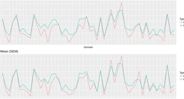
The proposed MSE is also working under the logarithmic transformation (see Figure 6 and Figure 14 in the appendix) . The estimated MSE tracks the empirical MSE well.
GB2 scenario
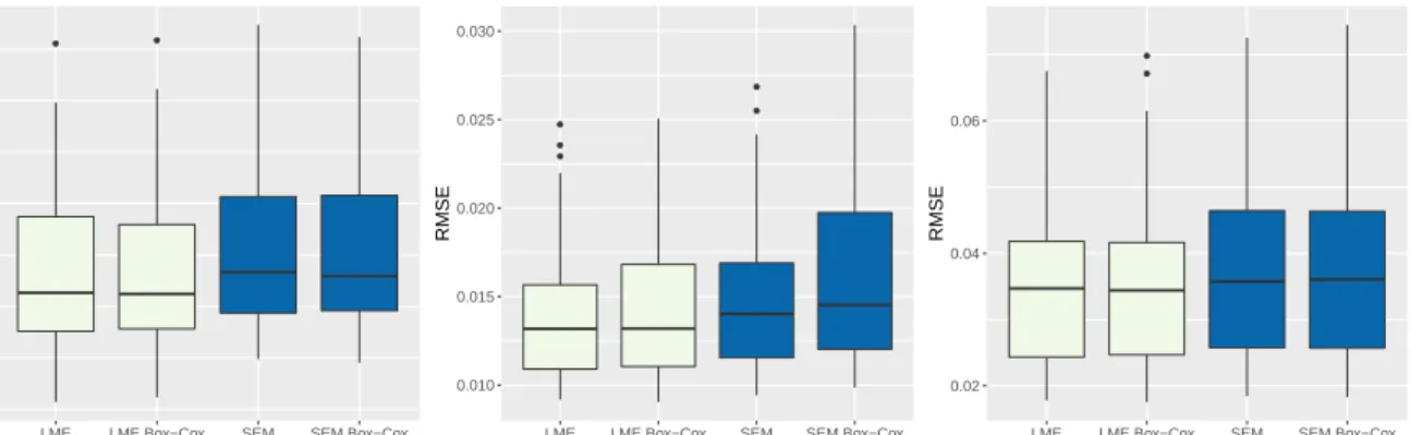
The dependent variable in the GB2 scenario is again censored to seven intervals (see Table 7 in the appendix). The results show (see Figure 7 and Table 8) that the RMSE of the Gini and HCR using the SEM algorithm is smaller compared to the RMSE using LME. While this seems counter-intuitive, one reason might be that the SEM-algorithm is robust against outliers and thus performs better in the case of skewed data. Furthermore, the results highlight the functioning of the Box-Cox transformation even when the data is grouped. Again the results are backed up by a density plot given in the appendix (see Figure 17). It is seen that the SEM Box-Cox method reconstructs the true distribution best, even though it is only using the interval informations.
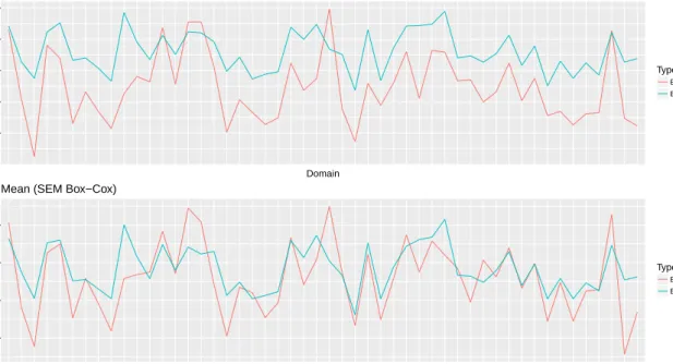
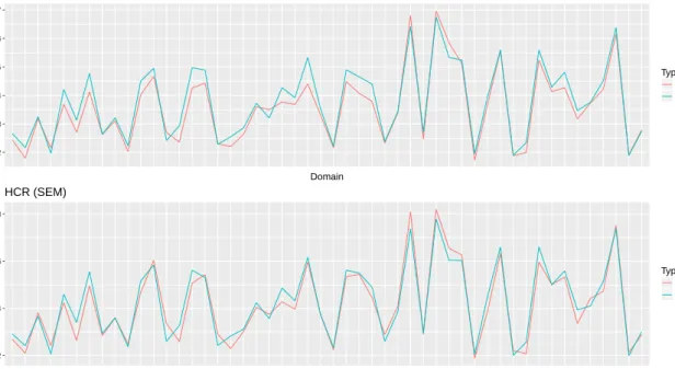
The Figures 8 and 16 in the appendix show, that the estimated RMSE is tracking the empirical RMSE well. Therefore the proposed bootstrap provides useful results even under the Box-Cox transformation.
750 1000 1250 1500 Domain RMSE Type Empirical Estimated Mean (LME Log)
800 1000 1200 1400 Domain RMSE Type Empirical Estimated Mean (SEM Log)
Figure 6: Log scenario, MSE for the mean.
● ● ● 300 400 500
LME LME Box−Cox SEM SEM Box−Cox
Method RMSE Mean ● ● 0.02 0.03 0.04
LME LME Box−Cox SEM SEM Box−Cox
Method RMSE Gini ● ● 0.03 0.04 0.05 0.06 0.07
LME LME Box−Cox SEM SEM Box−Cox
Method
RMSE
HCR
Figure 7: GB2 scenario, RMSE for the proposed methods.
6
Conclusion
The paper introduces a SEM-algorithm that estimates the parameter of a nested error linear regression model when the dependent variable is grouped. This enables the use of the popular EBP method, which is based on these models, when the target variable is grouped. The proposed SEM-algorithm relies on normally distributed error terms. Since this is rarely the case in applied work, transformations are in-corporated into the algorithm to handle departures from normality. Furthermore, an MSE estimation procedure that accounts for the additional variability, coming from the interval censored dependent vari-able, is proposed.
To validate the proposed estimation methods extensive model based simulations were performed using different scenarios. The simulation results validate the functioning of the proposed SEM-algorithm and show that in most scenarios the loss of accuracy in the EBPs, is minimal compared to the use of the uncensored data. That accuracy is lost is obvious, because only the group information, hence less information is used by the algorithm. The amount of accuracy lost in the EBPs using the SEM-algorithm compared to the use of the uncensored data, strongly depends on the number of intervals the data is censored to. In the GB2 scenario the EBPs using the SEM-algorithm even outperform the EBPs using the true uncensored data. A possible explanation is that the SEM-algorithm is robust against outliers. Finally, empirical evaluation also validate the functioning of the proposed parametric bootstrap, also under transformations.
350 400 450 500 550 Domain RMSE Type Empirical Estimated Mean (LME Box−Cox)
350 400 450 500 Domain RMSE Type Empirical Estimated Mean (SEM Box−Cox)
Figure 8: GB2 scenario, MSE for the mean.
Further research will focus on the robustness properties of the proposed methods against outliers and on inferential statistics.
7
Appendix
LME LMEBox SEM SEMBox
Mean 206.6279 206.0218 216.5873 214.7854
Gini 0.0132 0.0132 0.0140 0.0145
HCR 0.0347 0.0344 0.0357 0.0361
Table 3: Normal scenario 1, median RMSE for the proposed methods.
0.02 0.03 0.04 0.05 0.06 0.07 Domain RMSE Type Empirical Estimated HCR (LME) 0.02 0.04 0.06 Domain RMSE Type Empirical Estimated HCR (SEM)
Figure 9: Normal scenario 1, MSE for the HCR.
LME LMEBox SEM SEMBox
Mean 202.3627 205.5423 256.3309 254.2082
Gini 0.0133 0.0132 0.0156 0.0169
HCR 0.0349 0.0345 0.0392 0.0403
0.00000 0.00005 0.00010 0.00015 0.00020 0 2500 5000 7500 10000 Y Density Method LME LME Box−Cox SEM SEM Box−Cox
Figure 10: Normal scenario 1, predicted and true density.
Interval Frequencies [1,500) 1473 [500,1000) 1703 [1000,2000) 2113 [2000,4000) 2093 [4000,8000) 1453 [8000,16000) 770 [16000, Inf) 395
Table 5: Log-scale scenario, distribution for one arbitrary chosen population.
150 200 250 300 Domain RMSE Type Empirical Estimated Mean (LME) 200 250 300 350 Domain RMSE Type Empirical Estimated Mean (SEM)
0.02 0.03 0.04 0.05 0.06 0.07 Domain RMSE Type Empirical Estimated HCR (LME) 0.02 0.04 0.06 0.08 Domain RMSE Type Empirical Estimated HCR (SEM)
Figure 12: Normal scenario 2, MSE for the HCR
0.00000 0.00005 0.00010 0.00015 0.00020 0.00025 0 2500 5000 7500 10000 Y Density Method LME LME Box−Cox SEM SEM Box−Cox
Figure 13: Normal scenario 2, predicted and true density
LME Log LME Box-Cox SEM Log SEM Box-Cox
Mean 975.0483 974.6505 988.2902 991.2858
Gini 0.0344 0.0359 0.0353 0.0377
HCR 0.0646 0.0638 0.0672 0.0678
0.05 0.06 0.07 0.08 0.09 Domain RMSE Type Empirical Estimated HCR (LME Log) 0.06 0.07 0.08 0.09 0.10 Domain RMSE Type Empirical Estimated HCR (SEM Log)
Figure 14: Log scenario, MSE for the HCR.
0e+00 1e−04 2e−04 3e−04 0 10000 20000 30000 Y Density Method LME Log LME Box−Cox SEM Log SEM Box−Cox
Figure 15: Log scenario, predicted and true density.
Interval Frequencies [1,3000) 408 [3000,5000) 1361 [5000,7000) 2580 [7000,9000) 2554 [9000,11000) 1624 [11000,13000) 778 [13000, Inf) 695
LME LME Box-Cox SEM SEM Box-Cox
Mean 457.1321 416.0161 463.7191 429.3658
Gini 0.0434 0.0238 0.0258 0.0236
HCR 0.0635 0.0467 0.0395 0.0379
Table 8: GB2 scenario, median RMSE for the proposed methods.
0.035 0.040 0.045 0.050 0.055 Domain RMSE Type Empirical Estimated HCR (LME Box−Cox) 0.030 0.035 0.040 0.045 0.050 Domain RMSE Type Empirical Estimated HCR (SEM Box−Cox)
Figure 16: GB2 scenario, MSE for the HCR.
0e+00 5e−05 1e−04 0 10000 20000 30000 Y Density Method LME LME Box−Cox SEM SEM Box−Cox
References
Battese, G. E., Harter, R. M., and Fuller, W. A. (1988). An error component model for prediction of county crop areas using survey and satellite data. Journal of the American Statistical Association, 83 (401):28–36.
Bayes, T. (1763). An essay towards solving a problem in the doctrine of chances. by the late rev. mr. bayes, f. r. s. communicated by mr. price, in a letter to john canton, a. m. f. r. s. Philosophical Transactions, 53:370–418.
Box, G. E. P. and Cox, D. R. (1964). An analysis of transformations. Journal of the Royal Statistical Society. Series B (Methodological), 26(2):211–252.
Caleux, G. and Dieboldt, J. (1985). The sem algorithm: A probalistic teacher algorithm derived from the em algorithm for the mixture problem.Computational Statistics Quarterly, 2:73–82.
Chambers, R. and Tzavidis, N. (2006). M-quantile models for small area estimation. Biometrika, 93 (2):255–268.
Dempster, A., Laird, N., and Rubin, D. (1977). Maximum likelihood from incomplete data via the em algorithm.Journal of the Royal Statistical Society. Series B (Methodological), 39(1):1–38.
Draper, N. R. and Cox, D. R. (1969). On distributions and their transformation to normality. Journal of the Royal Statistical Society. Series B (Methodological), 31(3):472–476.
Elbers, C., Lanjouw, J. O., and Lanjouw, P. (2003). Micro-level estimation of poverty and inequality.
Econometrica, 71(1):355–364.
Foster, J., Greer, J., and Thorbecke, E. (1984). A class of decomposable poverty measures.Econometrica, 52(3):761–766.
Gini, C. (1912). Variabilit`a e mutabilit`a. Reprinted in Memorie di metodologica statistica (Ed. Pizetti E, Salvemini, T). Rome: Libreria Eredi Virgilio Veschi.
Gonzalez-Manteiga, W., Lombardia, M. J., Molina, I., Morales, D., and Santamaria, L. (2008). Analytic and bootstrap approximations of prediction errors under a multivariate fay-herriot model. Computa-tional Statistics & Data Analysis, 52 (12):5242–5252.
Graf, M., Nedyalkova, D., M¨unich, R., Seger, J., and Zins, S. (2011). Parametric estimation of income distributions and indicators of poverty and social exclusion. Advanced Methodology for European Laeken Indicators.
Hyndman, R. J. and Koehler, A. B. (2006). Another look at measures of forecast accuracy.International Journal of Forecasting, 22(4):679 – 688.
In-Known, Y. and Johnson, R. A. (2000). A new family of power transformations to improve normality or symmetry. Biometrika, 87(4):954–959.
Manly, B. F. J. (1976). Exponential data transformations.Journal of the Royal Statistical Society. Series D (The Statistician), 25(1):37–42.
McCullagh, P. (1980). Regression models for ordinal data.Journal of the Royal Statistical Society. Series B (Methodological), 42(2):109–142.
Molina, I. and Rao, J. N. K. (2010). Small area estimation of poverty indicators. The Canadian Journal of Statistics, 38 (3):369–385.
Pfeffermann, D. (2002). Small area estimation - new developments and directions. International Statis-tical Review, 70 (1):125–143.
Rao, J. and I.Molina (2015). Small Area Estimation. John Wiley & Sons, Inc.
Rojas-Perilla, N., Pannier, S., Schmid, T., and Tzavidis, N. (2017). Data-driven tansformation in small area estimation.
Statistisches Bundesamt (2017). Datenhandbuch zum mikrozensus scientific use file 2012. http://www.forschungsdatenzentrum.de/bestand/mikrozensus/suf/2012/
fdz_mz_suf_2012_schluesselverzeichnis.pdf. Accessed: 2017-07-22.
Stewart, M. (1983). On least square estimation when the dependent varaible is grouped. The Review of Economic Studies, 50(4):737–753.
United Nations (1995). The copenhagen declaration and programme of action. World Summit for Social Development.
United Nations (2017). Sustainable development goals. http://www.un.org/
sustainabledevelopment/. Accessed: 2017-07-22.