An Improved Robust Optimization Approach for Scheduling Under Uncertainty

(1)

AN IMPROVED ROBUST OPTIMIZATION APPROACH FOR SCHEDULING UNDER UNCERTAINTY

A Thesis by

UTKARSH DINESH SHAH

Submitted to the Office of Graduate and Professional Studies of Texas A&M University

in partial fulfillment of the requirements for the degree of MASTER OF SCIENCE

Chair of Committee, Efstratios N. (Stratos) Pistikopoulos Committee Members, Costas Kravaris

Phanourios Tamamis Head of Department, M. Nazmul Karim

August 2017

Major Subject: Chemical Engineering

(2)

ABSTRACT

In practice, the uncertainty in processing time data frequently affects the feasibility of optimal solution of the nominal production scheduling problem. Using the unit-specific event-based continuous time model for scheduling, we develop a novel multi-stage ro-bust approach with corrective action to ensure roro-bust feasibility of the worst case solution while reducing the conservatism arising from traditional robust optimization approaches. We quantify the probability of constraint satisfaction by using a priori and a posteriori probabilistic bounds for known and unknown uncertainty distributions, consequently, im-proving the objective value for a given risk scenario. Computational experiments on sev-eral examples were carried out to measure the effectiveness of the proposed method. For a given constraint satisfaction probability, the proposed method improves the objective value compared to the traditional robust optimization approaches.

(3)

DEDICATION

(4)

ACKNOWLEDGMENTS

I would like to thank Prof. Christodoulos A. Floudas under whose guidance I initiated my research project at Texas A&M University. It was his charismatic personality and passion that instill in me the basics of computational thinking.

I would like to thank my thesis advisor, Prof. Efstratios N. Pistikopoulos for his guid-ance in helping me finish my thesis successfully. I would also like to thank people on my committee, Prof. Costas Kravaris and Dr. Phanourios Tamamis. This work would not have been possible without academic supports from my lab mates, Dr Yannis Guzman, Logan Matthews and Wenjie Xu. I cannot imagine my time at Texas A&M University without the company of Justin Katz, William Tso, Melis Onel, Doga, Barris and Burcu Bekyal. Fi-nally, I would like to acknowledge my friends and family who provided me with constant motivation and emotional support.

(5)

CONTRIBUTORS AND FUNDING SOURCES

Contributors

This work was supported by a thesis committee consisting of Prof. Pistikopoulos and Prof. Kravaris of the Department of Chemical Engineering and Dr. Tamamis of the Energy Institute.

All other work conducted for the thesis was completed by the student independently.

Funding Sources

(6)

NOMENCLATURE Indices i, i′ Tasks j, j′ Units n, n′, n′′ Events s State u Utilities Sets I tasks

Ij task that can be performed in unitj

Is task that can process state s and either consume or pro-duce it

Ic_s task that consume state s

Ip_s task that produce state s

J units

Ji units suitable for performing task i

N event points within the scheduling horizon

S states

SP states that are final product

SR states that are raw materials

Parameters

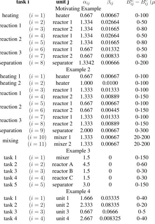
B_iL minimum capacity (batch size) of task i

B_iU maximum capacity (batch size) of task i

(7)

H short-term time horizon

M large positive number in big-M

N number of event points

Ps price of state s

ST_s0 initial amount of state s available

ST_smax maximum amount of state s

αi coefficient of constant term of processing time of task i

βi coefficient of variable term of processing time of task i ∆n maximum number of events over which taskiis allowed

to continue

ρis proportion of state s produced (ρis ≥ 0) or consumed (ρis ≤0) by taski

Binary Variable

winn′ binary variable for assignment of task i that starts at eventnand ends at eventn′

ωini′n′ binary variable for assignment of weight for task i′ fin-ished in eventn′ on taskiabout to occur inn(n > n′) Positive Variable

binn′ amount of material undertaking taskithat starts at event

nand ends at eventn′ (n′ ≥n)

ST0s initial amount of state s that is required from external resources

STsn excess amount of statesthat needs to be stored at event

n

T_inf time at which taskiends at eventn Ts

in time at which taskistarts at eventn

MIP Mixed Integer Program

(8)

TABLE OF CONTENTS

Page

ABSTRACT . . . ii

DEDICATION . . . iii

ACKNOWLEDGMENTS . . . iv

CONTRIBUTORS AND FUNDING SOURCES . . . v

NOMENCLATURE . . . vi

TABLE OF CONTENTS . . . viii

LIST OF FIGURES . . . x

LIST OF ALGORITHMS . . . xi

LIST OF TABLES . . . xii

1. INTRODUCTION . . . 1

1.1 Statement of Problem . . . 1

1.2 Outline of Thesis . . . 3

2. SHORT-TERM BATCH SCHEDULING FRAMEWORK . . . 4

2.1 Time Representations . . . 4

2.2 Mathematical Model . . . 6

2.3 Motivating Example . . . 11

3. ROBUST OPTIMIZATION . . . 13

3.1 Uncertain Inequality Constraints . . . 14

3.2 Uncertainty Sets . . . 16

3.3 Probabilistic Robust Optimization . . . 20

4. SCHEDULING UNDER UNCERTAINTY . . . 24

(9)

4.2 Reactive Scheduling: Improvements . . . 29

4.3 An Improved Robust Scheduling Approach . . . 33

4.4 Improving the quality of solution . . . 40

4.5 Computational Studies . . . 42

5. SUMMARY AND CONCLUSIONS . . . 44

5.1 Objectives Achieved . . . 44

5.2 Further Study . . . 45

REFERENCES . . . 46

(10)

LIST OF FIGURES

FIGURE Page

2.1 State-Task Network (STN) for motivating example . . . 12

2.2 Nominal Schedule for motivating example (H =8 hrs) . . . 12

4.1 Soyster Solution for bounded uncertainty case . . . 28

4.2 Solution with probability of constraint violation = 0.1 . . . 28

4.3 Reactive Scheduling Simulation . . . 31

4.4 Proactive-Reactive Scheduling Approach . . . 32

4.5 Improved Robust Scheduling Approach . . . 38

4.6 Improved Robust Soyster Solution . . . 39

(11)

LIST OF ALGORITHMS

ALGORITHM Page

3.1 Traditional Robust Optimization . . . 21

3.2 Iterative Approach for Robust Optimization . . . 23

4.1 Algorithm for Reactive Scheduling . . . 29

4.2 Algorithm for Proactive-Reactive Scheduling . . . 30

(12)

LIST OF TABLES

TABLE Page

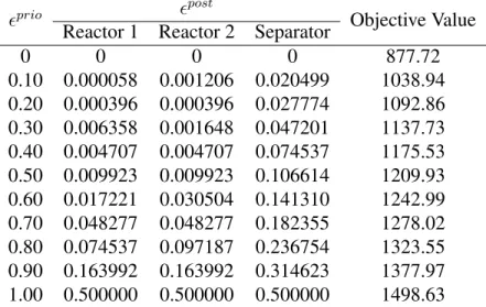
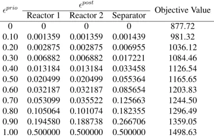
4.1 Improved Robust Approach for motivating example with interval-polyhedral set . . . 40 4.2 Improved Robust Approach for motivating example with interval-ellipsoidal

set . . . 41 4.3 Computational Study on Literature Benchmark . . . 43 A.1 Batch Size Data for motivating example and Examples 2-4 . . . 54

(13)

1. INTRODUCTION

Production scheduling is a decision-making process to determine what to produce, when to produce and how much to produce. Traditionally, these decisions are carried out by trained individuals without mathematical optimization using spreadsheets and gantt charts [1]. The increase in production volumes, product portfolios, alternative production recipes and energy cost has raised the complexity of manual scheduling. The later coupled with growing global competition and complexity of manufacturing facilities has made it essential to deploy effective optimization tools for generating most profitable and effort-less schedules.

In spite of the literary advances in process scheduling, the gap between academic research and industrial application of these optimization tools remains wide open. One of the pri-mary cause can be attributed to accounting for fundamental reality of uncertainty in pro-cessing parameters. The uncertainty in propro-cessing parameters can not only lead to delays in schedules but also lead to infeasibility for otherwise optimal solution [2] leading to decrease in operators confidence in the optimal schedule. In order to handle the critical re-ality of uncertainty in scheduling, we propose a multi-stage robust optimization approach with corrective action to ensure feasibility of the worst case solution while reducing the conservatism arising from traditional robust optimization.

1.1 Statement of Problem

The scheduling problem of chemical processes is defined as follows. Given:

i. production recipes (i.e. the processing times for each task at the suitable units, and the amount of the materials required for the production of each product),

(14)

iii. material storage policy, iv. production requirement, and

v. time horizon under consideration, Determine

i. the optimal sequence of tasks taking place in each unit,

ii. the amount of material being processed at each time in each unit, iii. the processing time of each task in each unit,

so as to optimize a performance criterion, for example, to minimize the makespan or to maximize the overall profit. The most common sources of uncertainty in the aforemen-tioned scheduling problem are:

i. the processing times of tasks,

ii. the market demands for products, and iii. the prices of products and/or raw materials.

The uncertainty in market prices and product demands manifest on the scale of 24-48 hrs, while the uncertainty in processing time parameters manifest on scale of few minutes to hours. Hence, from a context of short term scheduling with a typical time horizon of 8-16 hrs, processing time uncertainty has the maximum detrimental effect on operations. The uncertainty in processing time can be described using known or unknown, symmetric or asymmetric, continuous or discrete distributions. Note that, with increased knowledge about uncertain parameters distribution, we gain improved probabilistic guarantees on ro-bust solutions feasibility.

(15)

1.2 Outline of Thesis

The rest of this book is organized as follows. In Chapter 2, we briefly review the relevantliteraturein theareaofshort-termprocessschedulingand describeindetailsthe model used in this work. Chapter 3 provides a background on theory of robust optimization including the use of probabilistic bounds. Chapter 4 address the issue of scheduling under uncertainty and proposes a improved robust optimization formulation forschedulingunderuncertainty.

Finally, in the last chapter, wesummarize the contributionof the developmentsand pointoutavenuesforfutureresearch.

(16)

2. SHORT-TERM BATCH SCHEDULING FRAMEWORK

Scheduling is a important tool for production facilities, affecting the productivity and profitability of a facility. The problem of scheduling has received considerable attention in recent years from both academic and industrial research communities [1, 3] as it arises in almost any type of industrial production facilities (Pulp and paper, Metals, Oil and Gas, Pharmaceuticals, Food and Beverages, etc.). The objective of scheduling problem is to allocate optimal sequences and sizes of task to suitable units subject to availabil-ity of resource such as materials and utilities to meet market demands. Due to increase in complexity and flexibility of the production facilities, scheduling problem sizes vary from simple, single-stage processes to highly complicated, multi-product, multi-purpose processes. More thorough reviews on scheduling are presented by Floudas and Lin [3], Mendez et al. [4], Phanden et al. [5] and Maravelias [6].

2.1 Time Representations

Scheduling models can be broadly classified into two main categories based on time representations, namely, discrete-time and continuous-time models. Early attempts at pro-cess scheduling were based on discretization of time horizon into a finite number of time interval [7]. Since, the beginning and ending of tasks are associated with boundaries of these intervals, one needs to select intervals as small as greatest common factor of arbitrary processing times. Selecting such small interval often leads to extremely large problem size, especially for real world problems. Specific solution techniques and reformulation are employed to reduce the problem size and improve computational efficiency [8, 9]. Discrete-time methods are a relatively straightforward method to model timing constraints as they provide exact location of every time t in grid. This simplicity comes in handy when modeling the change in electricity prices and power availability [10, 11, 12].

(17)

How-ever, this simplicity comes at the cost of approximation of continuous nature of processing task durations and large number of binary variables corresponding to each discrete time interval.

To alleviate the inherent limitations of discrete-time models, continuous-time repre-sentation methods have been developed. Unlike discrete-time models where events are allowed to begin only at certain time intervals, continuous-time models allow event to be-gin at almost any time point. Continuous representation of time is captured by variable event times, or event points, which can be defined globally or on a unit-specific basis. A large number of inactive intervals of discrete-time models are eliminated by using vari-able time event points, thus, significantly reducing number of integer varivari-ables. However, additional variables and constraints has been defined to accurately model the timing and sequencing constraints, resulting in models with more challenging structures. As a re-sult, a significant amount of research has been dedicated to the development of efficient continuous-time formulations in past two decades.

Continuous-time models can be classified based on type of process representation, namely, sequential processes and general network-represented process. While sequential processes do explicitly consider mass balances as they are order- or batch-oriented, general network-represented processes can handle more general cases of mass splitting and merg-ing balances. Two groups of general network-represented models have been developed, slot based model and event based model. Ordered blocks or slot of unknown, variable lengths represents time horizon in slot based models. While on the other hand, continuous variables are directly defined to represent timings of tasks in event based models. Event based models can be further classified as global event-point and unit-specific event-point model. Global event based models [13] represent time horizon using a set of event (or time) points that are common for all tasks and in all units. In contrast, event points on a unit basis are defined in unit-specific models [14].

(18)

The unit-specific event based continuous-time formulation for short-term was origi-nally proposed by Floudas and coworkers [14, 15, 16, 17, 18, 19]. Event points are defined as a sequence of time instances located along time axis of each resource or unit, each rep-resenting the beginning of a task or utilization of a resource. Since the location of event points are different for different units, the tasks assigned to same event are allowed to start at different moments in different units. Due to this additional decomposition of event points for different units, for the same scheduling problem, the number of event points re-quired in the unit-specific event based formulation is smaller than the number of events in global event based models.For a scheduling problem, reduced number of binary variables that results from unit-specific event-based formulation, leads to smaller model sizes and efficient solutions for large-scale models.

2.2 Mathematical Model

Due to established advantages of unit-specific event-based models [20, 21], we use them as they lead to smaller number of binary variables and computationally efficient models. The work presented in this thesis is based on the continuous time unit-specific event-based deterministic model proposed by Floudas and co-workers. Note that the for-mulation presented below may differ from original publication, but in spirit, it is mathe-matical equivalent and identical with one found in Li and Floudas [22].

Allocation Constraints

Based on the original formulation, a three-index binary allocation variable winn′ is defined, to determine assignment of a task i that starts in event n and ends in event n′

(n ≤n′). ∑ i∈Ij ∑ n′∈N winn′ ≤1∀j ∈J, n∈N ∑ i∈Ij ∑ n∈N winn′ ≤1∀j ∈J, n′ ∈N (2.1)

(19)

Constraint 2.1 allows at most one task to begin (end) at an eventn(n′) in unitj. If a given task can be performed in multiple units, then the task is split into multiple tasks, each suitable in only one unit.

∑ n′∈N winn′ + ∑ i′∈Ij i′̸=i ∑ n′∈N wi′n′n≤1∀i∈Ij, j ∈J, n∈N (2.2)

Constraint 2.2 states that if a task starts in unitjat eventn, no other task in unitj can end at eventn. Only the task that begins at eventncan end at eventn.

∑ n′∈N winn′ ≤1− ∑ n′∈N n′<n ∑ n′′∈N ∑ i′∈Ij wi′n′n′′+ ∑ n′∈N n′<n ∑ n′′∈N ∑ i′∈Ij wi′n′′n′∀j ∈J, i∈Ij, n∈N, n >1 (2.3) Constraint 2.3 states that a task iin unitj can start at eventnonly if unitj is idle i.e. all tasksi′that started before eventnhave ended before eventn.

∑ n′∈N win′n≤ ∑ n′∈N n′≤n ∑ n′′∈N win′n′′− ∑ n′′∈N ∑ n′∈N n′<n win′′n′∀i∈I, n∈N (2.4)

Constraint 2.4 allows a task to end only if it had started earlier.

Capacity Constraints

B_iminwinn′ ≤binn′ ≤Bimaxwinn′∀i∈I, n, n′ ∈N (2.5) Batch size limitations are enforced by constraint 2.5

(20)

Material Balances STsn =STs(n−1)+ ∑ i∈Ips ρis ∑ n′∈N bin′(n−1)+ ∑ i∈Ic s ρis ∑ n′∈N binn′∀s ∈S, n∈N, n >1 (2.6)

In Constraint 2.6, the inventory of a state s at event n is adjusted by considering the inventory in previous event, amount generated in previous event and amount consumed starting from eventn.

STsn =ST0s+ ∑ i∈Ic s ρis ∑ n′∈N binn′∀s ∈S, n= 1 (2.7)

Constraint 2.7 accounts for initial inventory of the states.

Duration Constraints

T_inf ≥T_ins +αiwinn+βibinn∀i∈I, n∈N (2.8) Constraint 2.8 ensures that the finish time of a task is later than the sum of its start time and processing time.

T_inf ≥T_ins ∀i∈I, n∈N (2.9) Constraint 2.9 states that finish time of a task is later than its start time.

T_inf′ ≥Tins +αiwinn′ +βibinn′ −M(1−winn′)∀i∈I, n, n′ ∈N, n < n′ (2.10)

Constraint 2.10 adjusts the finish time of a task if the task is processed across multiple event points.

(21)

Sequencing Constraints T_i(n+1)s ≥T_inf∀i∈I, n∈N, n < N (2.11) T_i(n+1)s ≤T_inf +M [ 1−(∑ n′∈N n′≤n ∑ n′′∈N win′n′′− ∑ n′′∈N ∑ n′∈N n′<n win′′n′) ] +M ∑ n′∈N win′n∀i∈I, n∈N, n < N (2.12)

Constraint 2.11 states that start time of task in an event is later than finish time of task in previous event. If a task spans across multiple event points, a zero-wait condition is applied when the task ends in event later thann.

T_i(n+1)s ≥T_if′_n−M [ 1−(∑ n′∈N n′≤n ∑ n′′∈N wi′n′n′′− ∑ n′′∈N ∑ n′∈N n′<n wi′n′′n′) ] ∀i, i′ ∈Ij, i̸=i′, j∈J, n∈N, n < N (2.13)

Constraint 2.13 states that start time of a task in an unit has to be later than finish time of task that occurs in the same unit in previous event.

T_i(n+1)s ≥T_if′_n−M(1−

∑

n′∈N

wi′n′n)

(22)

For tasks that consume and produce the same state in different units, Constraint 2.14 en-forces the start time of consumption task to be later than finish time of production task.

Tightening Constraint ∑ i∈Ij ∑ n∈N ∑ n′∈N (αiwinn′ +βibinn′)≤H∀j ∈J (2.15) Sum of processing times for all the tasks that take place in a unit should be less than the scheduling horizon.

Bounds on Variable

T_ins ≤H, T_inf ≤H∀i∈I, n∈N (2.16)

winn′ = 0, binn′ = 0∀i∈I, n, n′ ∈N, n′ < n (2.17)

Objective Function

Several different objective functions can be employed for sort-term scheduling prob-lems. Two most common types are reviewed below.

Maximization of Profit max Profit =∑ s∈S Ps ∑ n=N (STsn+ ∑ i∈Ips ρis ∑ n′∈N bin′n) (2.18)

(23)

Alternatively, one can optimize the time taken by a schedule (a.k.a. makespan) to meet given demands of products. Minimization of Makespan

min MS ∑ n=N (STsn+ ∑ i∈Ips ρis ∑ n′∈N bin′n)≥Ds∀s ∈S T_iNf ≤M S∀i∈I (2.19)

Note that, if using minimization of makespan as objective, replace time horizonH with makespanM Sin the model. Also, additional constraints like utility balance, intermediate due dates, storage considerations, etc. can be added to the model.

2.3 Motivating Example

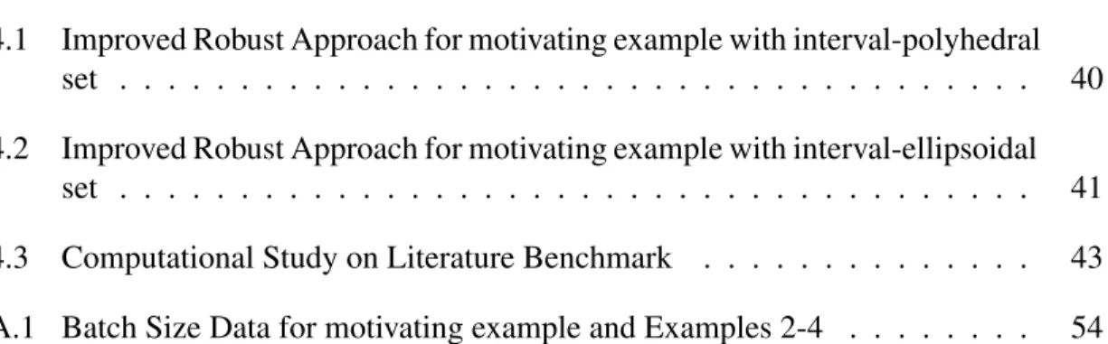
The study was performed on the standard benchmark example originally introduced by Kondili et al [7]. In figure 2.1, statess1,s2ands3represent the raw materials. While

s2 and s3 can be directly used in reaction 2 i2, i3, s1 needs to be under go heating i1 in the heater j1. States s4, s5, s6 and s7 are the intermediate products of the reaction scheme that produces final products as statess8 ands9. All the reactions can take place in two reactor units j2 and j3, hence mathematically reaction in one reactor is treated differently than that in other reactor. Eg., reaction 1 is broken into two tasks i2 and i3 that take place in reactor 1j2and reactor 2j3respectively. The data for parameters can be found in appendix. Nominal schedule for profit maximization problem with 8 hrs as its time horizon is showed below. Note that for above problem, we use 4 events points as determined by Li and Floudas [22].

(24)

Figure 2.1: State-Task Network (STN) for motivating example. Reprinted with permission from [22]. Copyright c⃝2010 American Chemical Society.

0 1 2 3 4 5 6 7 8 Hours Heater Reactor1 Reactor2 Seperator 70.21 40.51 64.81 45.39 22.13 72.62 35.4 34.04 54.46 88.5 Objective=1498.630000

Heating Reaction1 Reaction2 Reaction3 Seperation

(25)

3. ROBUST OPTIMIZATION

The efficacy of a mathematical model relies on the accuracy of information fed to the model in form of parameters. Typically, these parameter values exhibit uncertainty in data due to limited information or measurement error. The solution of such a mathematical model with uncertain parameter values would vary greatly based on which values are re-alized by these uncertain parameter. One of the methods to immunize the mathematical models against uncertainty is Robust Optimization. These is done by ensuring feasibility of the constraints for any possible realization of parameter points in uncertainty sets. These uncertainty sets are defined by deterministic data of parameter realization. The problem that corresponds to feasible solution for uncertainty set is also called robust counterpart.

Earliest work in robust optimization was published by Soyster [23], formulating the so-called "worst-case" robust counterpart, where the problem is immunized against all possible perturbations of data. The Soyster solution to a problem would ensure that no possible realization of uncertain parameter would render the solution infeasible. However, if the uncertain parameters take unbounded distributions, it is impossible to generate a Soyster solution for which probability of constraint violation is zero for any realization of uncertain parameter. Thus, it is desirable to generate solutions and quantify the trade-off between robustness and performance. The interval + ellipsoidal uncertainty set and a method to provide upper bound on constraint violation probability for given set was proposed by Ben-Tal and Nemirovski [24, 25]. A linear robust counterpart method was introduced by Bertsimas and Sim [26], as they proposed and characterized interval + poly-hedral uncertainty set. The robust optimization framework was extended to mixed-integer linear programs(MILPs) by Floudas and coworkers [2, ?, 27, 28] with parameters sub-ject to uncertainty with known or unknown distributions, including unbounded probability

(26)

distributions.

Traditionally, the quality of a robust solution relies on strength ofa priorimethods that define uncertainty sets which satisfy a upper bound on probability of constraint violation or a lower bound on probability of constraint satisfaction. A tighter probabilistic bound would allow for improvement in objective value for a given risk, thus leading to a less con-servative solution. A priorimethods were characterized by Ben-Tal and Nemirovski [25] and Bertsimas and Sim [29] for interval + ellipsoidal and interval + polyhedral uncertainty sets, respectively. These bounds were extended to apply to other variety of uncertainty sets and various distributions of uncertainty by Floudas and coworkers [30, 31, 32, 33, 34]. Alternatively, one can characterize the probability of constraint violation of a solution, namely,a posterioribounds on constraint violation, which are stronger thana prioribound of equivalent structure. A nonconvex optimization problem is generated whena posteriori bounds are incorporated in robust counterparts instead of using uncertainty sets. To avoid solving a nonconvex optimization problem and to take advantage of tighter a posteriori bounds, Li and Floudas [31] proposed an iterative method to obtain improved solution for a particular risk tolerance. Compared to both worst-case solution and traditional one-pass robust optimization framework, a dramatic improvement in solutions can be obtained by utilizing tightera priorianda posterioribounds along with the iterative framework.

3.1 Uncertain Inequality Constraints

Methods for generating robust counterparts of deterministic models have been devel-oped to apply on cases, where uncertain parameters are involved in linear or mixed-integer linear inequality constraints. In practice, these forms can often be achieved with simple substitutions or reformulations. Given arbitrary functionfi(x, y)participating in constraint

(27)

i, wherexandyare continuous and integer variables respectively: fi(x, y) + ∑ k aikxk+ ∑ l bilyl+ ∑ m pim≤0 (3.1)

Assume that the exact values of some or all of parametersaik, ∀k,bil, ∀landpim, ∀mare uncertain. An equivalent reformulation of constraint 3.1 is:

fi(x, y) +ti ≤0 −ti+ ∑ k aikxk+ ∑ l bilyl+ ∑ m pim≤0 (3.2)

A similar reformulation can be applied to an objective function with uncertain parameters. The general form of LP or MIP under uncertainty is as follows:

max x,y ∑ k ˜ ckxk+ ∑ l ˜ dkyk s.t. ∑ k ˜ aikxk+ ∑ l ˜ cilyl ≤p˜i ∀i yl ∈ {0, 1} ∀l (3.3)

Any parameter denoted with tilde is a parameter subject to uncertainty. The solutions and objective value of Model 3.3 changes for different realization of uncertain parameters.

(28)

Similar to3.1→ 3.2reformulation, we can equivalently express model 3.3 as follows: max x,y,z z s.t. z−∑ k ˜ ckxk− ∑ l ˜ dkyk ≤0 ˜ pix0+ ∑ k ˜ aikxk+ ∑ l ˜ cilyl ≤0 ∀i x0 =−1 yl∈ {0, 1} ∀l (3.4)

Generically, the uncertain inequality constraintican thus be represented as:

∑ j /∈Ji aijxj + ∑ j∈Ji ˜ aijxj ≤bi (3.5)

where,˜aij represents uncertain parameters whose indicesjare in setJi. xj can be contin-uous, integer or fixed variable to accommodate right hand side parameter uncertainty.

3.2 Uncertainty Sets

Selection of the uncertainty sets are central to formulating the robust counterpart. Un-certainty set, Ui is a deterministic set of multiple possible parameter realizations that is going to be imposed on the constraint i. Similar to behavior of guaranteed constraint feasibility when parameters realize their fixed values, constraint feasibility can be guaran-teed if thetruerealization of parameter values is contained within the uncertainty set. An uncertain parameteraij can be rewritten as function of random variableξij:

˜

(29)

where, ¯aij is the constant nominal or expected value of˜aij and ˆaij is a positive constant. Random variableξij captures the random realizations of ˜aij. For a bounded uncertainty, value of ˆaij should be chosen such that˜aij ∈ [¯aij −aˆij, ¯aij + ˆaij], in other words,ξij ∈ [−1, 1]. The uncertainty setUi can be defined as set of realizations ofξi that meet some criteria, whereξiis a vector of all random perturbations of parametersj ∈Ji.

Various kinds of norm-based uncertainty sets have been defined in the literature. These norm-based uncertainty sets are conic convex and will help develop robust counterparts as seen further in this chapter.

A box uncertainty set can be defined using a∞-norm distance fromξi =0.

U_i∞= { ξi :∥ξij∥∞= max j∈Ji |ξij|≤Ψi } (3.7)

where the size of U_i∞ is controlled by parameter Ψi. Geometrically, U_i∞ represents a hypercube. If the uncertainty is bounded, selecting Ψi = 1 will include all possible realization of uncertainty, thus representing the worst-case uncertainty set. Typically, when Ψi = 1,Ui∞is also referred as interval uncertainty set.

A polyhedral uncertainty set can be defined using a1-norm distance fromξi =0.

U_i1 = { ξi :∥ξij∥1= ∑ j∈Ji |ξij|≤Γi } (3.8)

where the size ofU1

i is controlled by parameterΓi. Geometrically,Ui1 represents a poly-hedron. For bounded uncertainty, selectingΓi =|Ji|will include all possible realizations of uncertainty as well as some spurious ones (when|Ji|>1) inUi1.

A ellipsoidal uncertainty set can be defined using a2-norm distance fromξi =0.

U_i2 = { ξi :∥ξij∥2= ∑ j∈Ji |√ξ2 ij|≤Ωi } (3.9)

(30)

where the size of U2

i is controlled by parameterΩi. Geometrically, Ui2 represents a ellip-soid. For bounded uncertainty, selectingΩi =

√

|Ji|will include all possible realizations of uncertainty as well as some spurious ones (when|Ji|>1) inUi2.

As observed, for bounded uncertainty, utilizing1-norm or2-norm based uncertainty sets, can lead to inclusion of realizations of uncertainty which have zero probability of occur-rence due to the uncertainty set geometries. In order to alleviate this, interval uncertainty set is intersected with other norm-based criteria. Intersecting1-norm and interval set leads to a interval+polyhedral set: U_i1∩∞ = { ξi :∥ξij∥1= ∑ j∈Ji |ξij|≤Γi,∥ξi∥∞≤1 } (3.10)

where, the size of set is controlled byΓi. For bounded uncertainty set, setting Γi = |Ji| will ensure that all realization of uncertainty are included inU_i1∩∞. Similarly, intersecting 2-norm and interval set leads to a interval+ellipsoidal set:

U_i2∩∞ = { ξi :∥ξij∥2= ∑ j∈Ji |√ξ2 ij|≤Ωi,∥ξi∥∞≤1 } (3.11)

where, the size of set is controlled byΩi. For bounded uncertainty set, settingΩi =

√

|Ji| will ensure that all realization of uncertainty are included inU2∩∞

i .

In order, to utilize a given uncertainty setUionto constrainti, we reformulate constraint 3.5 using 3.6, ∑ j ¯ aijxj+ ∑ j∈Ji ξijˆaijxj ≤bi (3.12) and now ensure maximal feasibility of the constraint for all realizations of setUi,

∑ j ¯ aijxj + max ξi∈Ui { ∑ j∈Ji ξijˆaijxj } ≤bi (3.13)

(31)

The inner maximization problem is conic convex and exhibits strong duality. Utilizing du-ality theory, inner maximization problem can be replace by a deterministically equivalent minimization problem, thus generating a robust counterpart of constraint 3.5. The robust counterpart of constraint 3.5 subject to a box uncertainty set is:

∑ j ¯ aijxj + Ψi ∑ j∈Ji ˆ aij|xj|≤bi (3.14)

The robust counterpart of constraint 3.5 subject to a polyhedral uncertainty set is:

∑ j ¯ aijxj + Γizi ≤bi zi ≥aˆij|xj| ∀j ∈Ji (3.15)

The robust counterpart of constraint 3.5 subject to a ellipsoidal uncertainty set is:

∑ j ¯ aijxj + Ωi √∑ j∈Ji ˆ a2 ijx2j ≤bi (3.16)

The robust counterpart of constraint 3.5 subject to a interval + polyhedral uncertainty set

is: _∑ j ¯ aijxj+ ∑ j∈Ji pij + Γizi ≤bi zi+pij ≥ˆaij|xj| ∀j ∈Ji pij ≥0 ∀j ∈Ji zi ≥0 (3.17)

The robust counterpart of constraint 3.5 subject to a interval + ellipsoidal uncertainty set is: ∑ j ¯ aijxj + ∑ j∈Ji ˆ aij|xj −zij|+Ωi √∑ j∈Ji ˆ a2 ijzij2 ≤bi (3.18)

(32)

3.3 Probabilistic Robust Optimization

The size of an uncertainty set can be controlled using parametersΨi, Γi, orΩi, which can be generically referred to as∆i. For bounded uncertainty case, it is possible to include all realizations of ξi in Ui by setting ∆i value to its maximum values (Ψi = 1, Γi =

|Ji|, orΩi =

√

|Ji|), thus rendering the probability of constrainti’s violation to zero for any realization ofξi. Pr { ∑ j ¯ aijxj + ∑ j∈Ji ξijˆaijxj > bi : ξij ∈[−1, 1], ∆i = ∆ (max) i } = 0 (3.19)

Alternatively for unbounded uncertainty case, to include every possible realization, the value of parameter ∆i must approach infinity. Also, for either bounded or unbounded case, imposing every possible realization leads to extremely conservative solutions. A reduction in ∆i value leads to less conservative solution at an expense of probability of constraint violation being non-zero.

Pr { ∑ j ¯ aijxj + ∑ j∈Ji ξijˆaijxj > bi : ξij ∈[−1, 1], ∆i <∆ (max) i } >0 (3.20)

Say that we have acceptable risk appetite of constrainti’s violation ϵprio_i . We can set∆i a priori such that regardless of optimal solution x∗, we can guarantee that probability of constraint violation is utmost ϵprio_i . A priori probabilistic bounds are the probabilistic expressionB(∆i)that relate probability of constraint violation to∆i. As this bounds must work regardless of the solution, they provide upper bounds on probability of constraint violation: Pr { ∑ j ¯ aijxj + ∑ j∈Ji ξijˆaijxj > bi } ≤B(∆i) =ϵprioi (3.21)

(33)

Solutions become less conservative for smaller values of∆i, hence minimum value of∆i should be selected such thatB(∆i)≤ϵprioi . Formulating an optimization problem:

min ∆i ∆i s.t. B(∆i)≤ϵprioi ∆i ≥0 (3.22)

In order to obtain tightest possible solution of model 3.22, one needs tighta prioribound

B(∆i). A traditional robust optimization approach can be derived utilizinga prioribounds. Alternatively, one can quantify the probability of constraint violation a posteriori for a

Algorithm 3.1Traditional Robust Optimization

Require: Provide Deterministic model M, select uncertainty set type U? _and _{A priori}

probability of constraint violationϵprio_i ∀i∈I procedureAPRIORIROBUSTOPTIM(M, U?, ϵprio)

MRC ←M

for alli∈I do ◃For each constraint with uncertain parameters

MRC ←robustCounterpartGen(MRC, Ui?) ◃Generates Robust Counterpart ∆i ←aPrioriBound(ϵprioi ) ◃Solution of model 3.22

end for

x∗ ←optimizationSolver(MRC, ∆)

returnx∗, MRC, ∆ ◃Retrieve Robust Optimal Solution and robust counterpart

model

end procedure

optimal solution x∗. Similar to a priori bounds, one can define a posteriori bounds as probabilistic expressionB(x∗)which relate probability of constraint violation tox∗:

Pr { ∑ j aijx∗j + ∑ j∈Ji ξijˆaijx∗j > bi } ≤B(x∗) = ϵpost_i (3.23)

(34)

For a given x∗, a tighter a posteriori bound B(x∗)will assign lower probability of con-straint violationϵpost_i . Utilizinga posterioribounds, Li and Floudas [31] proposed alterna-tive method to calculate robust solution. They proposed a following approximate model:

min x,∆i cx s.t. −∆i(bi− ∑ j ¯ aijxj) + ∑ j∈Ji lnE[e∆iξijaˆijxj_]≤_ln_ϵpost i ∀i ∆i ≥0 ∀i (3.24)

As observed, model 3.24 is non-convex optimization problem and requires deterministic global optimization approach to obtain the optimal solution. The increased objective value from usinga posterioribounds comes at an expense of computational power. To mitigate this increase in computational expense, they proposed an alternative method for utilizing a posterioribounds: Needless to mention, tighta priorianda posterioribounds help re-duce the number of iterations for alg. 3.2 and improve the objective value of the solution. Recently, Floudas and coworkers [32, 33, 34] proposed novel a priori and a posteriori bounds and characterized them to be the strongest bounds proposed in literature to date. In this work, the bounds are generated by PROTO [35], which relies on these recently pro-posed novel bounds. Since the bounds generated by PROTO are for independent random parameters, we assume the parameters follow independent random distributions.

(35)

Algorithm 3.2Iterative Approach for Robust Optimization

procedureITERATIVEROBUSTOPTIM(M, U?, ϵ)

Set tolerance parameterδ(e.g. 0.01)

x∗, MRC, ∆satisf y ←AprioriRobustOptim(M, U?, ϵ) ◃From alg. 3.1 ∆ = ∆satisf y

for alli∈I do ◃For each constraint with uncertain parameters

ϵpost_i ←posterioriProb(M, x∗) ◃Using equation 3.23

while|ϵpost_i −ϵi|> δ do ifϵpost_i ≤ϵi then ∆satisf y_i = ∆i else ∆violate_i = ∆i end if ∆i ←0.5(∆violatei + ∆ satisf y i ) x∗ ←optimizationSolver(MRC, ∆i)

ϵpost_i ←posterioriProb(M, x∗) ◃Using equation 3.23

end while end for

returnx∗ ◃Retrieve Robust Optimal Solution witha posterioriprobability of

constraint voilationϵ end procedure

(36)

4. SCHEDULING UNDER UNCERTAINTY

Scheduling problems are inherently plagued with fundamental reality of uncertainty in processing time parameters, market prices, resources and unit availability, or product demands. Most of the literary advances in area of process scheduling has ignored this fundamental reality and proposed nominal-case schedules. Upon realization of uncertain parameters during operation, these nominal schedules often cause delay or infeasibility of schedules, leading to confusion on the operation floor.

Typically, there are two approaches for scheduling under uncertainty: reactive ap-proach and preventive apap-proach [36]. In reactive scheduling, nominal schedules are gen-erated and updated upon the realization of uncertainty. Generation of new schedules is based on feedback of realized states to the scheduler. These approaches tend to be com-putationally expensive, since uncertainty can occur frequently and optimization problems have to be solved repetitively. Since reactive scheduling relies on rescheduling of nominal problem upon realization of uncertainty, feasibility of solution cannot be guaranteed. In order to alleviate computational issues and improve feasibility of the solution, reschedul-ing algorithms often employ heuristics or decomposition approach.

Earliest approaches in reactive scheduling were based on decision tree analysis [37]. The decision trees were generated by introducing artificial errors to the execution and then the heuristic chose a reschedule decision such that impact on original schedule is mini-mal. To avoid future infeasibility, look-ahead procedures were introduced by Rodrigues et al [38]. Mendez and Cerda proposed general MILP reactive scheduling approach for multi-purpose batch plants with limited changes in batch sequencing and units for smooth rescheduling. Penalty incurred by rescheduling actions were incorporated in objective value by Kopanos et al [39]. Similar methods for reactive scheduling were proposed in the

(37)

literature [40, 41]. Reactive scheduling models often employ novel techniques to enhance feasibility, minimize disruption and reduce computational efforts due to rescheduling.

In contrast, proactive scheduling approaches generate schedules prior to realization of parameters by incorporating a deterministic model of uncertainty in the optimization problem. Proactive scheduling ensures that the solution remains feasible for all possible realizations of uncertainty at the cost of detriment in objective value. One of the promi-nent approaches for proactive or preventive scheduling is robust optimization. Floudas and coworkers [2, 42] extended robust optimization framework to MILP problem and devel-oped robust scheduling approach. As described in previous chapter, robust optimization does not require explicit knowledge of probabilistic models for uncertainty.

Robust scheduling usually suffers from conservatism and large deterioration in objec-tive value. To overcome this problem, adjustable robust optimization (ARO) framework was proposed by Ben-Tal et. al. [43] Since only a subset of decision have to take place "here-and-now", many decisions can be delayed until later point. This holds true especially for scheduling problem as, only the batch-size and sequence of task needs to decided here-and-now, while the time to start a task can be decided later on realization of uncertainty. Instead of obtaining a single, static optimal solution, ARO framework aims at obtaining an optimal policy that is parameterized in realizations of uncertainty. Effectively, with respect to process scheduling literature, ARO approach can be designated as a cross between re-active and prore-active scheduling. Often, these decision based on parameter realizations are assigned using heuristic. Shi and You [44] applied ARO framework to batch scheduling by formulating a 2-stage problem from deterministic MILP model. This model requires computationally expensive techniques to obtain solution and is limited to cases where all uncertain information is revealed before any second stage decision is taken. A multi-stage ARO approach for scheduling problem was proposed by Lappas and Gounaris [45]. They generated a robust counterpart of continuous-time global event point model for scheduling

(38)

by incorporating a decision-dependent uncertainty set. In interest of numerical tractability, they used a heuristic affine relationship for event time decision rules:

Tn ←[Tn]0+ ∑ i∈I ∑ n′<n [Tn]in′αin′ (4.1)

where, αin′ is an uncertain parameter. Through case studies, they demonstrated an im-provement in objective value from ARO method when compared to traditional robust op-timization method for an arbitrary size of uncertainty set. The disadvantages of ARO are use of heuristic decision rules, increase in computational size of model and absence of any probabilistic bounds on the solution.

More thorough reviews on scheduling under uncertainty are presented by Li and Ier-apetritou [36], Verderame et al. [46] and, Dias and IerIer-apetritou [47].

4.1 Traditional Robust Scheduling Approach

As demonstrated by ARO approaches, a combination of proactive and reactive solution strategies would lead to improved objective values while ensuring feasibility of schedule. As describe in state of problem, for short-term scheduling problem we consider uncertainty in processing time parameters. Also, for demonstration purposes we consider uncertainty to be uniform and boundα˜i = [0.7 ¯αi,1.3 ¯αi]. Note that, one can handle uncertainty in raw material or resource availability, market prices or demand as well, but for demonstration purposes we consider processing time parameters as the only uncertainty. We assume that uncertain parameters are randomly independent.

(39)

constraints 2.8 and 2.10 contain the uncertain parameterαi1:

T_inf ≥T_ins + ˜αiwinn+βibinn∀i∈I, n∈N

T_inf′ ≥Tins + ˜αiwinn′ +βibinn′−M(1−winn′)∀i∈I, n, n′ ∈N, n < n′

Substitutingα˜i = ¯αi+ξiαˆiin constraint 2.8 and 2.10 and maximizing the effect of uncer-tainty for a unceruncer-tainty set.

T_inf ≥T_ins + ¯αiwinn+βibinn+ max ξin∈Uin

{αˆiξinwinn}∀i∈I, n∈N (4.2)

T_inf′ ≥Tins+ ¯αiwinn′+βibinn′−M(1−winn′)+ max ξin∈Uin

{αˆiξinwinn′}∀i∈I, n, n′ ∈N, n < n′ (4.3) Where, α¯i is the expected or nominal value of parameter α˜i andαˆ is a positive constant. Since, cardinality of uncertainty setUinis 1, choosing either box, polyhedral or ellipsoidal sets would make no difference. The robust counterpart can be written as:

T_inf ≥T_ins + ¯αiwinn+βibinn+ ∆in{αˆiwinn}∀i∈I, n∈N (4.4)

T_inf′ ≥Tins + ¯αiwinn′+βibinn′−M(1−winn′) + ∆in{αˆiwinn′}∀i∈I, n, n′ ∈N, n < n′ (4.5) For bounded uncertainty case, setting ∆in = 1would lead to worst-case (a.k.a. Soyster) solution. Alternatively, nominal scheduled can be achieved by setting ∆in = 0. Any intermediate value of∆inwould lead to a solution with non-zero probability of constraint violation.

1_{Note that tightening constraint 2.15 contains uncertain parameter}_α

i, but for demonstration purposes we

drop that constraint from the model. Since the constraint was redundant the model feasibility and solution is unaffected.

(40)

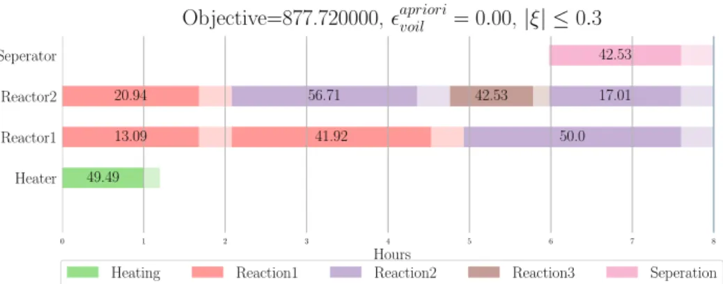
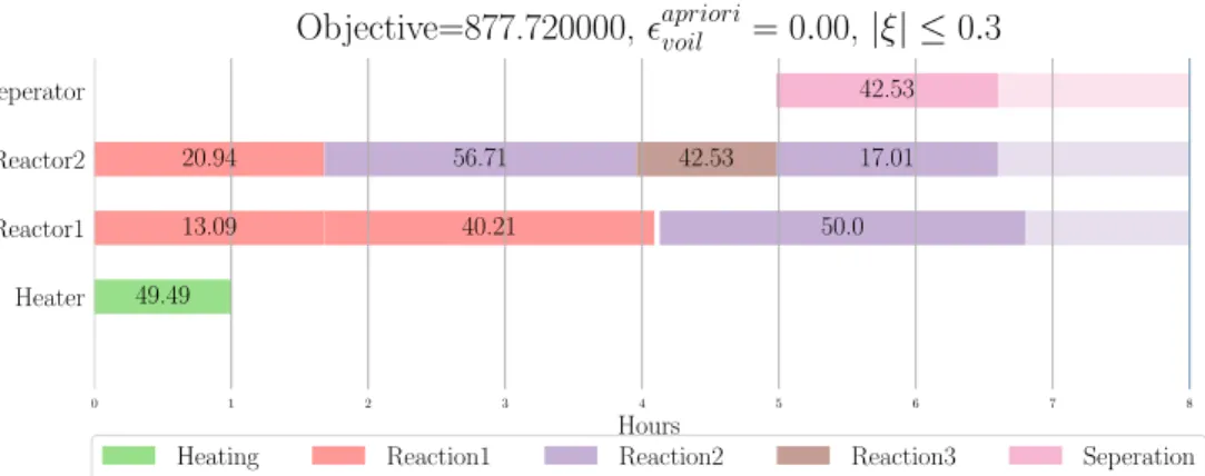
Now replacing, constraints 2.8 and 2.10 with their robust counterparts 4.4 and 4.5 in the model from chapter 2 and solving the optimization problem for motivating example, we obtain: where, the transparent shade is the extra time allotted to a task to account for

0 1 2 3 4 5 6 7 8 Hours Heater Reactor1 Reactor2 Seperator 49.49 13.09 41.92 20.94 50.0 56.71 42.53 17.01 42.53

Objective=877.720000,apriori_voil = 0.00, |ξ| ≤0.3

Figure 4.1: Soyster Solution for bounded uncertainty case

0 1 2 3 4 5 6 7 8 Hours Heater Reactor1 Reactor2 Seperator 28.81 14.05 24.73 39.56 27.7 13.51 44.33 21.61 20.78 33.25 54.02

Objective=914.820000,apriori_voil = 0.10, _|ξ_{| ≤}0.3

Figure 4.2: Solution with probability of constraint violation = 0.1

uncertainty. Now consider the unit reactor 1, tasks occurring in this unit are independent to tasks in other units.

(41)

Since, the feasibility of each task in Reactor 1 i.e. probability of constraint satisfaction of each task in Reactor 1 is1−ϵprio _{= 0}_.₉_{, the overall probability of feasible operation} of Reactor 1 is (1−ϵprio₎4 _{= 0}_.₆₅_{. Thus the actual probability of feasible operation of a} single unit is much less than that desired. Extending this observation to multiple units and the actual feasibility of complete schedule would exponentially reduce, in practice, such a schedule with reduced feasibility is unacceptable. Although, it is worth noting that robust scheduling model has not added any additional variables or constraint to the problem and has not lead to any increase in problem size.

4.2 Reactive Scheduling: Improvements

On the other hand, if we were to resort to reactive scheduling approach and reschedule after realization of uncertainty at every event point. To achieve this reactive scheduling behavior, we created following algorithm.

Algorithm 4.1Algorithm for Reactive Scheduling

procedureREACTIVESCHEDULING(M, ξU B)

x∗ ←NominalScheduler(M) ◃Using deterministic model of Chapter 3

for alln ∈range(1, N −1)do ◃e.g. 4 event points in motivating example

w_innf x′ ←winn∗ ′∀n′ ≥n ◃Fix task assignment of eventn

bf x_inn′ ←b∗inn′∀n′ ≥n ◃Fix batch size of eventn

αin ←randUniform((1−ξU B)αin,(1 +ξU B)αin) ◃A random value is assigned to processing time of tasks in event n

x∗_n←x∗ ◃Store intermediate solution

x∗ ←NominalScheduler(M) ◃Updated model is re-optimized,winn′ andbinn′ are fixed

end for

returnx∗_n ◃Retrieve all the solutions

(42)

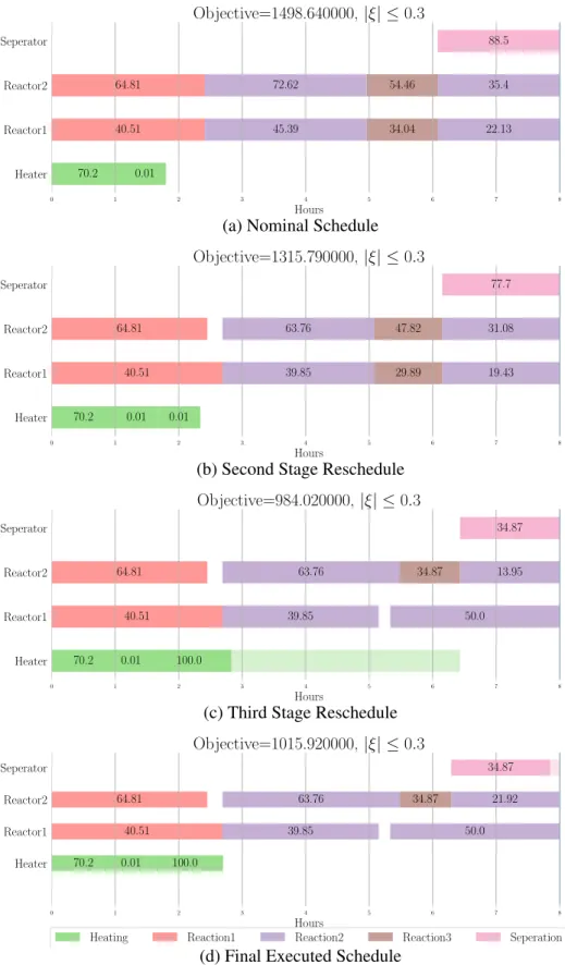
As observed from example simulation (fig. 4.3), the objective value of the overall schedule over the horizon is not guaranteed. Due to constant rescheduling, it leads to confusion on production floor. In order to take advantage of improvement in objective value that comes from using algorithm 4.1, while maintaining schedule feasibility we pro-pose a proactive-reactive scheduling approach. In this approach, we modify algorithm 4.1 to generate robust solution for each stage instead of nominal schedule.

Algorithm 4.2Algorithm for Proactive-Reactive Scheduling

procedurePROREACTIVESCHEDULING(MRC, ξU B, ϵprio) ◃Using deterministic model of Chapter 3 coupled with constraints 4.4 and 4.5

x∗ ←AprioriRobustOptim(MRC, ξU B, ϵprio) ◃Robust solver from algorithm 3.1

for alln ∈range(1, N −1)do ◃e.g. N = 4event points in motivating example

bf x_inn′ ←b∗_inn′∀n′ ≥n ◃Fix batch size of eventn

αin ←randUniform((1−ξU B)αin,(1 +ξU B)αin) ◃A random value is assigned to processing time of tasks in event n

x∗ ←AprioriRobustOptim(MRC) ◃Updated model is re-optimized,

winn′ andbinn′ are fixed

end for

end procedure

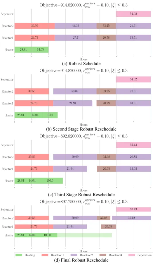
Observing the simulation example (fig. 4.4) for algorithm 4.2, the rescheduling deci-sion are not drastic as compared to algorithm 4.1. This modification results in improved feasibility and practical applicability of method at cost of objective value deterioration.

(43)

0 1 2 3 4 5 6 7 8 Hours Heater Reactor1 Reactor2 Seperator 70.2 0.01 40.51 64.81 45.39 22.13 72.62 35.4 34.04 54.46 88.5 Objective=1498.640000,_|ξ_{| ≤}0.3

(a) Nominal Schedule

0 1 2 3 4 5 6 7 8 Hours Heater Reactor1 Reactor2 Seperator 70.2 0.01 0.01 40.51 64.81 39.85 19.43 63.76 31.08 29.89 47.82 77.7 Objective=1315.790000,|ξ| ≤0.3

(b) Second Stage Reschedule

0 1 2 3 4 5 6 7 8 Hours Heater Reactor1 Reactor2 Seperator 70.2 0.01 100.0 40.51 64.81 39.85 50.0 63.76 34.87 13.95 34.87 Objective=984.020000,|ξ| ≤0.3

(c) Third Stage Reschedule

0 1 2 3 4 5 6 7 8 Hours Heater Reactor1 Reactor2 Seperator 70.2 0.01 100.0 40.51 64.81 39.85 50.0 63.76 34.87 21.92 34.87 Objective=1015.920000,|ξ| ≤0.3

(d) Final Executed Schedule

(44)

(a) Robust Schedule

0 1 2 3 4 5 6 7 8 Hours Heater Reactor1 Reactor2 Seperator 28.81 14.04 0.01 24.73 39.56 21.94 13.51 50.09 21.61 20.78 33.25 54.02

(b) Second Stage Robust Reschedule

0 1 2 3 4 5 6 7 8 Hours Heater Reactor1 Reactor2 Seperator 28.81 14.04 100.0 24.73 39.56 21.94 13.03 50.09 20.85 20.05 32.08 52.13

(c) Third Stage Robust Reschedule

Objective=897.750000,apriori_voil = 0.10, |ξ| ≤0.3

(d) Final Robust Reschedule

(45)

4.3 An Improved Robust Scheduling Approach

Although the feasibility of solution has improved, the resources and skill to re-optimize a schedule at every occurrence of uncertainty is not feasible on a complex production floor. We improve algorithm 4.2, by introducing new constraints in the model at every stage in rescheduling. Referencing to algorithms 4.1 and 4.2, we define each event point of information collection from simulation or feedback as the active event point.

T_inf ≥T˜_ins + ˜αinwinn+βibinn∀i∈I, nis the active event point (4.6)

T_inf′ ≥T˜ins+ ˜αinwinn′+βibinn′−M(1−winn′)∀i∈I, n′ ∈N, n < n′, nis the active event point (4.7) Where,T˜s

inis the uncertain start time of a task at eventn. This constraints are only intro-duced for an active event pointn. Uncertainty in start time of task is induced from uncer-tainty in processing parameters of task that occurred in previous events (α˜in′′∀ n′′ < n). Hence we can derive an expression forT˜s

inas a function ofα˜in′′. ˜ T_ins =T_isn+∑ i′∈I ∑ n′<n |ωin|i′n′αˆi′n′ξi′n′ (4.8)

where, T_ins is the value of start time if all parameters in the problem realize their nominal values. |ωin|i′n′ is a binary variable which decides whetherαi′n′ has any influence on the next event or not. Combining constraint 4.6 and 4.7, substituting 4.8 and generating robust

(46)

counterpart with Interval + Polyhedral uncertainty set using equation 3.17: T_inf′ ≥Tins +αinwinn′+βibinn′ + Γinzin+ ∑ i′∈I ∑ n′′∈N n′′<n |pin|i′n′+p′in

−M(1−winn′)∀i∈I, n′ ∈N, n≤n′, nis the active event point

zin+p′in ≥αˆinwinn′ ∀i∈I, n, n′ ∈N, n≤n′

zin+|pin|i′n′≥αˆi′n′|ωin|i′n′ ∀i, i′ ∈I, n′ ∈N, n′ < n, nis the active event point (4.9) where, zin, p′in and|pin|i′n′ are auxiliary positive variables introduced as a part of robust counterpart formulation. The big-M condition in constraint 4.9 will ensure that the con-straint is redundant ifwinn′ is inactive.

|ωin|i′n′≤wi′n′′n′∀i, i′ ∈I, n′, n′′ ∈N, n′′ ≤n′, n′ < n, nis the active event point (4.10)

|ωin|i′n′= 0∀i, i′ ∈I, n′, n′′∈N, n′ ≥n, nis the active event point

∑

i′∈I

∑

n′∈N n′<n

|ωin|i′n′≤n−1∀i∈I, nis the active event point

∑ i′∈I ∑ n′∈N n′<n |ωin|i′n′≤M ∑ n′∈N n′≤n

win′n∀i∈I, nis the active event point

(4.11)

Constraint 4.10 states that uncertainty in task that did not occur cannot influence start time of any task in future. Constraint 4.11 ensures that the uncertainty in future task has no influence on the start time of current task. Also, the maximum number of events that can affect the start time of a task cannot be more than the number of event points that have elapsed in the schedule so far. If a task is not suppose to start, then no past event can have

(47)

any influence on its start time. ∑ i′∈I ∑ n′∈N n′<n |ωin|i′n′αˆi′n′ ≥ ∑ i′∈Ij ∑ n′∈N n′<n ∑ n′′∈N n′′≤n′ ˆ αi′n′wi′n′′n′ −M(1− ∑ n′∈N n′≤n

win′n)∀i∈Ij, j ∈J, nis the active event point (4.12)

Constraint 4.12 asserts that the uncertainty in start time of a task is contributed from un-certainty in processing time of previous tasks in the same unit. Using inequality along with big-M constraint instead of equality, helps us ensure that there is no influence of uncertainty of tasks in previous event, if the current task is not performed.

∑ i′∈I ∑ n′∈N n′<n |ωin|i′n′αˆi′n′ ≥ ∑ i′∈Ij′ ∑ n′∈N n′<n ∑ n′′∈N n′′≤n′ ˆ αi′n′wi′n′′n′ −M(2− ∑ n′∈N n′≤n win′n −∑ i′∈Ips i′∈I_j′ ∑ n′∈N n′≤n

wi′n′(n−1))∀s∈S, i∈Ij, i ∈Ics, j, j′ ∈J, j′ ̸=j, nis the active event point

(4.13) Constraint 4.13 states that uncertainty in start time of a task is also contributed from un-certainty in processing time of tasks in a unit where, the raw material for current task was produced. Together, constraint 4.12 and 4.13 ascertain that uncertainty in start time of a task, is maximum of sum of processing time uncertainty in the same unit or in a depen-dent different unit. Grouping constraints 4.9, 4.10, 4.11, 4.12 and 4.13 intoMIR

n group of constraints for every active event pointn.

Compared to algorithm 4.2, here in algorithm 4.3, we fix αin to its nominal value instead of a random value. We add the MIR

n for each active event point. In comparison to previous reactive scheduling algorithms, this algorithm does not require any form of

(48)

Algorithm 4.3Algorithm for Improved Robust Scheduling

procedureIMPROBUSTSCHEDULING(MRC, ξU B, ϵprio) ◃Using deterministic model of Chapter 3 coupled with constraints 4.4 and 4.5

x∗ ←AprioriRobustOptim(MRC, ξU B, ϵprio) ◃Robust solver from algorithm 3.1

for alln ∈range(2, N)do ◃e.g. N = 4event points in motivating example

αi(n−1) ←α¯i(n−1) ◃Processing time values of elapsed events is fixed to their nominal value i.e. they behavior is changed from uncertainty parameter values to fixed values

∆i(n−1)←0 ◃Since the parameters are not uncertain anymore

MRC ←MRC+MnIR ◃Adding group of constraints from improved robust formulation

x∗ ←AprioriRobustOptim(MRC) ◃Updated model is re-optimized,

winn′ andbinn′ are fixed

end for

end procedure

on-line rescheduling. Once the schedule is generated, task assignment, sequencing and batch sizes remain unchanged, only the start times of tasks are affected by the uncertainty in processing time parameter.

Although, compared to traditional robust optimization problem, we need to solveN

instances of the scheduling problem. It must be noted that, every subsequent problem has lower number of binary decision variables as well as they start with a feasible solu-tion derived from previous solusolu-tion instance. Since, the structure of nominal scheduling model was unaltered by these robust counterpart formulation, any objective function or constraints such as makespan minimization, resource balance, intermediate due date, etc. can be applied on the model.

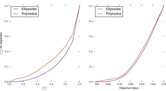
Figure 4.5 and 4.6 are two example instances solved using improved robust scheduling approach. As observed, the objective value has improved compared to both traditional robust scheduling and proactive-reactive scheduling for case with ϵprio _̸_{= 0}_{. While for}

(49)

worst case, there is no improvement in objective value. If one were to solve withϵprio _{= 1}_, the solution would be same as nominal schedule. Instead of using heuristic to determine start time of each task, we can logically determine the start time of each task as finish time of previous dependent task.

Alternatively, one can generate a robust counterpart for constraint 4.6 and 4.7 using Interval + Ellipsoidal Set. Also, for unbounded uncertainty case, one can generate a robust counterpart using polyhedral or ellipsoidal uncertainty sets.

T_inf′ ≥Tins +αinwinn′ +βibinn′ + Ωintin+ ∑ i′∈I ∑ n′′∈N n′′<n |uin|i′n′+u′in

−M(1−winn′)∀i∈I, n′ ∈N, n≤n′, nis the active event point

|uin|i′n′≥αˆi′n′|ωin|i′n′−|zin|i′n′ ∀i, i′ ∈I, n′ ∈N, n′ < n, nis the active event point

−|uin|i′n′≤αˆi′n′|ωin|i′n′−|zin|i′n′ ∀i, i′ ∈I, n′ ∈N, n′ < n, nis the active event point

u′_in ≥αˆinwinn′ −zin′ ∀i∈I, n, n′ ∈N, n≤n′, nis the active event point

−u′_in ≤αˆi′n′winn′ −zin′ ∀i∈I, n, n′ ∈N, n≤n′, nis the active event point

t2_in ≥(z_in′ )2+∑ i′∈I

∑

n′∈N n′<n

(|zin|i′n′)2∀i∈I, n∈N, nis the active event point (4.14) where,tin,z_in′ ,u′_in,|zin|i′n′ and|uin|i′n′ are introduced as positive auxiliary variables. The robust counterpart 4.14 is structured differently than one presented in constraint 3.18 but in spirit they are the same. These different reformulation follows a second order conic programming (SOCP) structure and can be solved using commercial MIP solvers like CPLEX and Gurobi [48] to global optimality (convex problem).

(50)