ISSN: 2088-8708 246
Energy-Efficient Multi-SPEED Routing Protocol for Wireless
Sensor Networks
Babak Namazi*, Karim Faez*
* Department of Electrical Engineering, Amirkabir University of Technology
Article Info ABSTRACT
Article history: Received Feb 3, 2013 Revised Mar 21, 2013 Accepted Mar 29, 2013
Wireless Sensor Networks (WSN) consists of a large number of sensor nodes randomly deployed in an area of interest to collect information from the environment. Due to lack of resources, energy efficiency and Quality of Service (QoS) are challenging issues in WSNs. In This paper, a new localized routing protocol is proposed which considers different QoS requirements in WSN. For latency considerations, it takes into account multiple levels of delay requirements by implementing different speed layers. Reliability needs are met by dynamically adjusting the transmission power of the sender and based on the energy consumed at the transmitter and the residual energy of the receiver, the forwarding decision is made. Finally, the performance of the protocol is evaluated using computer simulation.
Keyword: Energy efficiency Quality of service Routing
Wireless sensor networks
Copyright © 2013 Institute of Advanced Engineering and Science. All rights reserved.
Corresponding Author: Babak Namazi,
Department of Electrical Engineering, Amirkabir university of technology, Tehran, Iran.
Email: [email protected]
1. INTRODUCTION
Wireless sensor networks (WSNs) [1] consist of a large number of low-price sensor nodes capable of sensing and transmitting information from an area of interest. These sensors are equipped with low-power transceivers and communicate each other in an ad hoc fashion forming a multi-hop transmission mechanism to deliver the data to the destination node (sink). WSNs have had great application in recent years such as traffic monitoring, health care and other surveillance systems.
In spite of the great potential of WSNs, there are some restrictions in designing a communication protocol for these networks., such as limitations in energy, memory, bandwidth and reliability (because of the lossy nature of wireless links). Therefore, there is a need to find some protocols which takes all of these restrictions into account.
One of the most challenging issues of WSN is the design of a routing protocol which can meet the requirements of the application while considering the limitations of such networks. Some of the important challenges in designing a routing protocol are:
1. Energy efficiency: Due to battery limitation, the most important issue in WSN is the energy consumption. The packets should be transmitted to the destination using the least energy possible. In addition, in order to increase the network lifetime, the energy consumption has to be distributed over the whole network.
2. Quality of service: Supporting QoS is an important task in a routing protocols. This includes real-time communication, reliable transmission and resource reservation. Packets should be transmitted as soon as possible over the most reliable link while considering bandwidth constraints.
3. Diversity: According to the application, there might be various requirements for different flows. This is another factor that should be considered during a routing decision.
4. In addition, the forwarding protocol should have little overhead and be able to bypass the void areas in the network. It also should have enough flexibility to some network dynamics such nodes failure.
In this paper, we try to introduce a new localized geographic routing protocol which considers QoS in both time and reliability domain. For real-time communication, we use different speed layers, each aimed to guarantee a specific speed requirement and for reliability, we apply a power control approach to dynamically adjust the transmission power level. Based on the energy consumed at the transmitter and the remaining energy of the receiver, the forwarding node is selected among the nodes satisfying the QoS requirements.
The rest of the paper is organized as follows: In section 2, the related works are reviewed. Section 3, introduces the system model used. The proposed protocol is described in section 4 and is evaluated through simulation in section 5. Finally, section 6 concludes the paper.
2. RELATED WORKS
There exist many routing protocols for wireless ad hoc and sensor networks [2], [3]. Among all of these protocols, Greedy Forwarding [4] seems the most suitable, due to it's low overhead and high flexibility. In this method, the next hop is selected among the neighboring nodes which have an advance towards the sink. This is done based on the location of the neighboring nodes and the sink. Therefore, there is no need to save the complete path in the routing table.
Many researchers have worked on QoS routing protocols. Some of them are aimed for designing a real-time or reliable protocol while others consider both. As an example, SPEED [5] is a real-time routing protocol which tries to route the packet guaranteeing a fixed speed all over the network. The speed is checked locally at each hop and a back-pressure mechanism is used to move around the voids. This protocol does not consider multiple latency requirements and reliability is not mentioned in the routing policy. MMSPEED [6] is another routing protocol which uses multi-SPEED approach to form different speed layers each supporting a fixed speed. The latency is estimated locally, without additional packet transmission, and using IEEE 802.11e [7] as the MAC layer and a priority queuing method, the packets of different requirements are isolated. For reliability support, it uses multi-path approach which sends duplicated packets in case of an unreliable link. However, this method is not energy efficient due to the waste in sending the duplicated packet. Furthermore, multiple copies of the packet may cause congestion near the sink. The other drawback of the mention protocols is that they do not take energy into account in choosing the next hop.
In order to avoid packet duplication in reaching reliability requirements, we use a transmission power control approach. While increasing the transmission power leads to more reliable links and higher range for transceivers, decreasing it produces less interference for other nodes listening to the node. This technique has been used in routing by many researchers. As an example, ES-AODV [8] finds the minimum transmission power by dividing the desired received power by the signal decay. However, this protocol does not take into account the interference at the receiving node. In [9] an interference aware routing protocol is proposed. It tries to route the packet in the path which have less interference and consumes less energy. None of these protocols are localized routing protocols and therefore are not useful for wireless sensor networks.
In this work, we introduce a localized routing protocol which uses the information of the neighboring nodes to choose the next hop. We applied multi-SPEED approach to reach different latency requirements and based on the average interference of the receiver, the minimum transmission power that meets the reliability requirements is found. Using the remaining energy at the receiver node, we try to increase the lifetime of the network by avoiding energy depletion of some nodes in a more desirable path. In other words, our work extends MMSPEED protocol by adding energy efficiency using transmission power control.
3. SYSTEM MODEL
We applied a wireless sensor network consisting of a large number of sensor nodes randomly deployed in an area of interest. All of the sensor nodes have the same ability except for the sink node which has no energy limit. Nodes are assumed to be stationary or have little motion and know the location of the sink. The location of each node is also known to it by using a localization method.
We assume that a topology control protocol [10] has been applied to the network and each node has an initial transmission power level. This transmission power may vary for each transmission at anytime during network lifetime.
Each node can calculate the receiving power of a receiving packet as well as the Signal to Noise Ratio (SNR). The Bit Error Rate (BER)value can be calculated from SNR value according to the modulation used [11]. For example, in case FSK, the BER is:
2
2
1
SNRe
BER
(1)For wireless link we use log-normal multi-path model. The signal path loss for distance d is calculated as [11]: X d d d PL d PL ) ˆ ( log 10 ) ˆ ( ) ( 10 (2)
Where
d
ˆ
is the reference distance,
is the path loss exponent and Xis Gaussian random variable with mean zero and variance2. All of the variables are in deci-Bell.
All of the nodes can estimate their remaining energy at anytime during the network lifetime. In order to do this, we use the model in [12], in which the consumed energy is found by the sum of the time the node is in each state such as (sending, receiving and etc) multiplied by the power consumption for that state.
The consumed energy for transmitting the packet of size fis [12]:
) ( 8 ) ( tr P tr cir tr tr P P BW f P E (3)
in which BW is the bandwidth of the transceiver,
P
ciris the circle power and
is the conversion efficiency of the amplifier.We use the MAC used in MMSPEED which is a modified version of IEEE802.11e standard. However, in our protocol we do not need the modifications on the RTS/CTS exchange for a multicast transmission. In fact, we just use the IEEE802.11e standard with the ability to estimate the delays.
4. PROTOCOL OVERVIEW
In this section, the proposed protocol is described in details. At first, the required information is exchanged between the nodes and the routing table is formed. Using the required information, the sender checks the available nodes over their supporting speed and then, the proper transmission power is calculated for the eligible nodes. Finally, based on the energy consumed for transmission and the residual energy of the nodes the next hop is selected.
3.1. Neighbor Management
Like most of the geographic routing protocols, we need to exchange the required information between neighboring nodes. This is done by using Hello packets. These packets are broadcasted by all of the nodes in the network at fixed interval. This interval can be adjusted according to the mobility of the nodes; the more the nodes move the faster the information is exchanged to compensate the changes. The information needed to be transferred consists of the nodes' ID, location and mean interference. The mean interference value is calculated in each node when they receive a packet. This can be done by using the SNR value and the received signal strength. We use a moving average method like EWMA to count the value for all of the receptions.
Upon receiving such information from a node, nodes add an entry to their routing table and put the information there for further use.
3.2. Speed Calculation
When a node has a packet to be sent to the destination, it has to calculate the speed of the available node. The same method is used in MMSPEED to calculate this value. We have multiple speed layers and based on the required speed of the packet, a speed layer is assigned. Then, the nodes are checked over their latency and advance towards the sink. Based on this estimation, the nodes which have the ability to support the required speed can be found.
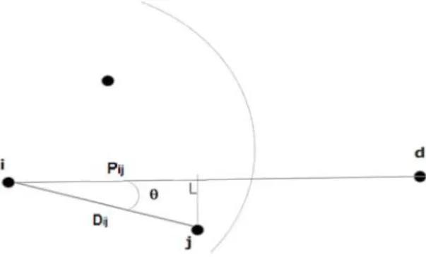
Figure 1. Greedy forwarding
Like MMSPEED, we assume that we have different preset values for speed layers called SetSPEED. When a node wants to send a packet, it checks the remaining time of the packet and based on the remaining time, the minimum speed layer that meets the requirement is chosen. Each speed layer is nothing but a queue and a traffic category at MAC layer.
Having the required speed layer, we need to check the neighboring nodes over their speed. In order to do this, we use the progress of the node in the line connecting the sender and the destination node which is a more realistic metric. This is shown in Figure 1. For example, for node i with coordinates
(
x
i,
y
i)
and the sink with coordinates(
x
d,
y
d)
, the progress of node j with position(
x
j,
y
j)
is found by the projection ofpoint j into line connecting i and d and is shown as
P
ijin Figure 1. The value ofP
ijis calculated as:
cos
ij ijD
P
(4)Where
D
ijis the distance between node i and j and
is the angle between lines ij and id. These are computed as: 2 2 ) ( ) ( i j i j ij x x y y D (5) 2 1 2 1 1 arctan m m m m (6)in which
m
1andm
2 are the sloop of line ij and line id respectively.i j i j x x y y m 1 (7) i d i d x x y y m 2 (8)
The speed for node j is found as:
ij ij ij delay P Speed (9)
In some cases, there might be more than one node satisfying the speed requirement. In such scenarios, we need to keep all of the eligible nodes to have the opportunity for load balancing and prevent energy depletion for a node. For this purpose, nodes satisfying the required speed form the set of fast nodes called FN. These nodes are checked over the reliability requirements in the next step.
3.3. Transmission Power Estimation
In this step, we use a power control method to reach the requirements in reliability domain. In order to do that, each node changes it's transmission power level to rectify an unreliable link. The metric for the reliability of a link is the BER value which can be estimated from the received packet's SNR.
As was mentioned earlier, nodes calculate the interference of a received packet and taking the history of all received packets, they have an estimation of the mean interference occurred during an interval of a Hello exchange. This information is broadcasted via Hello packets and by the use of this information, nodes will be aware of the interference their neighboring nodes might have. Thus, nodes with a packet to be sent can predict the SNR of the received packet and find the transmission power level at which they will send the packets.
When a node wants to forward a packet to the sink, it knows at which Packet Reception Ratio (PRR) the packet should be received at the destination. Therefore, for a node which has packets to be forwarded, the required PRR if node j is selected as the next hop is:
Pij Did PRR j prr / 1 ) ( (10)
According to the required packet reception ratio for node j we can calculate the maximum BER allowed in ij transmission. For packet of size f the packet reception ratio is:
f e j P j prr 8 )) ( 1 ( ) ( (11)
in which
P
e(
j
)
is the probability of bit errors in transmitting the packet from node i to j and is equal to the BER value. So the required BER for ij transmission would be:f j prr j BER 8 1 ) ( 1 ) ( (12) so we have: Pij Did f PRR j BER 8 / 1 1 ) ( (13)
Having the required BER for the next hop, we can calculate the required SNR based on the modulation used. Using the formula we have:
) 2 2 log( 2 ) ( 8 / 1 id ij D P f PRR j SNR (14)
The SNR value us computed at the receiver by subtracting the interference value by the received signal power. As was mentioned earlier, nodes are aware of the mean interference value occurred in the last interval of Hello exchange. Therefore, the required received power is found as:
) ( ) ( ) (j SNR j X j Prec (15)
in which X(j) is the average interference at node j. Having the required SNR, nodes can compute the required transmission power as:
) ( ) ( ) ( rec ij tr ij P j PL D P (16) so we have: X d D d PL j X PRR ij Ptr f Pij Did ij ) ˆ ( log 10 ) ˆ ( ) ( ) 2 2 log( 2 ) ( 8 / 10 1 (17)
It is noteworthy that the above formula is for the case FSK is used as the modulation type. The transmission power estimation is done for all of the eligible nodes in FN set which can support the required
speed. In this step, nodes which have the required transmission power more than the maximum transmission power level allowed for the transceiver are eliminated from this set. The remaining nodes are then checked over energy metrics to find the next hop.
3.4. Forwarding Policy
Having all of the nodes which can support the speed requirements and finding their corresponding transmission power, we can choose the next hop based on the energy needed for transmission and the remaining energy of the forwarding nodes. In order to do this, nodes are given a score according to the two energy metrics and based on this score the probability of the next hop selection will be found.
The required energy for transmission is found based on the transmission power level defined for the nodes and the remaining energy is transmitted by the Hello packets. Therefore, the score value for each node is: )) ( ( . ) ) ( ( . ) ( Norm E j ij E P Norm j Sc res tr ij (18)
Where
and
can be adjusted by the network requirements. The term)
(
ij
E
P
tr ijshows the progress made by consuming the required energy consumption for transmitting the packets from i to j. The normalized values can be calculated as:
FN k tr ik tr ij tr ij ik E P ij E P ij E P Norm ) ( ) ( ) ) ( ( (19)
FN k res res res k E j E j E Norm ) ( ) ( )) ( ( (20)The probability of selecting a specific node is calculated by dividing the score value of the node by the sum of the score values for all of the eligible nodes.
By considering both the consumed energy and the remaining energy of the nodes, we have an energy efficient transmission and avoid energy depletion for a single node or nodes from a single path.
5. SIMULATION RESULTS
In this section the performance of the proposed protocol, hereafter we call it EMSPEED (Energy-efficient Multi-SPEED), is evaluated through simulation. In order to do that, we use Castalia3.2 [13] simulator which is a suitable simulator for wireless sensor networks. We compare our protocol with the well-known MMSPEED protocol over different QoS metrics such as packet reception ratio and packet's latency and energy consumption. The simulation configurations are given in Table 1.
Table 1. Simulation configurations
Parameters value
Simulation area 200*200m2
Number of nodes 121
Deployment type Randomized grid
Sink location (200,200)
Source location (0,0)
Traffic rate 32Kbit/sec
Hello packet interval 100s
Simulation time 600s
bandwidth 200Kb/sec
Figure 2 shows the latency of received packets for different reliability requirements. It can be seen that MMSPEED has higher latency for higher reliability requirements. This is due to the duplication process which leads to more congestion in the network, especially near the sink, and therefore the delay is more. However, the latency in the proposed protocols does not have a significant increase. The little increase in latency in the proposed protocol is the result of selecting longer (hop-wise) but more reliable paths.
Figure 2. Latency of received packets for different PRRs
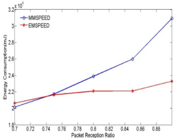
Figure 3. Energy consumption for different PRRs
The consumed energy for transmitting and receiving the packets for various PRR requirements is given in Figure 3. Since in MMSPEED protocol, we may have more than one transmission in sending the packets, the energy consumption increases with higher reliability requirements and it can be seen that EMSPEED protocol uses less energy than MMSPEED. The increase in energy consumption for EMSPEED protocol is due to the higher transmission power chosen for higher PRR requirements.
In Figure 4 the end-to-end packet reception ratio for various packet deadlines is shown. In MMSPEED protocol, for higher latency requirements, we have less reliable links and the packet is duplicated and sent through different path. Consequently, more congestion happens near the sink and more packets will be dropped because there may not be any nodes fulfilling the speed requirements. However, EMSPEED can choose farther node to reach the requirements and rectify the link by adjusting the transmission power and therefore, can support the latency requirement for different packets deadlines.
Figure 4. Packet reception ratio for different packets deadline
Figure 5. Energy consumption for different packets deadline
The energy consumption for different packets deadline is shown in Figure 5. As mention earlier, for higher latency requirements MMSPEED has more transmissions and this leads to higher energy consumption. It is clear that the proposed EMSPEED protocol consumes less energy for various packet deadlines.
In sum, it can be seen that the proposed EMSPEED can provide more reliability and less latency in comparison to MMSPEED protocol. Furthermore, for higher QoS requirements such latency and packet reception ratio, the energy consumption of the protocol does not vary significantly and can support different QoS needs with lower energy consumption.
6. CONCLUSION
In this paper, a new localized QoS routing protocol is proposed. It supports different latency requirements by choosing different speed layers and the reliability is met by dynamically adjusting the transmission power level. Considering both the consumed energy at the sender node and the remaining energy of the receiver, the next hop is chosen. Finally, we compared the protocol with the well-known MMSPEED protocol, and simulation results show that our protocol outperforms MMSPEED in terms of latency, reliability and energy consumption.
REFERENCES
[1] IF Akyildiz, W Su, Y Sankarasubramaniam, E Cayirci. Wireless sensor networks: a survey. Computer Networks. 2002; 38(4): 393-422.
[2] E Alotaibi, B Mukherjee. A survey on routing algorithms for wireless Ad-Hoc and mesh networks. Computer Networks. 2012; 940-965.
[3] K Akkaya, M Younis. A survey on routing protocols for wireless sensor networks. Ad-hoc Networks. 2005; 325-349. [4] B Karp, HT Kung. Gpsr: Greedy perimeter stateless routing for wireless networks. Proc. ACM MobiCom, 2000;
243-254.
[5] T He, JA Stankovic, TF Abdelzaher, C Lu. A spatiotemporal communication protocol for wireless sensor networks.
IEEE Transaction on Parallel and Distributed systems. 2005; 16(10): 995–1006.
[6] E Felemban, L Chang-Gun, E Ekici. Mmspeed: multi-path multi-speed protocol for qos guarantee of reliability and timeliness in wireless sensor networks. IEEE Transaction on Mobile Computing. 2006; 5(6): 738–754.
[7] Amendment8. Medium access control (mac) quality of service (qos) enhancements. IEEE Std 802.11e. 2005. [8] Wang X, Liu Q, Xu N. The energy-saving routing protocol based on AODV.Fourth International Conference on
Natural Computation. 2008.
[9] S Bhattacharya, S Bandyopadhyay. An Interference Aware Minimum Energy Routing Protocol for Wireless Networks Considering Transmission and Reception power of Nodes. Procedia Technology. 2012; 4: 1-8.
[10]A Aziz, Y Sekercioglu, P Fitzpatrick, M Ivanovich. A survey on distributed topology control techniques for extending the lifetime of battery powered wireless sensor networks. IEEE Communications Surveys and Tutorials.
2011; 99: 1–24.
[11]AF Molisch. Wireless Communication. John Wiley and sons, 2011.
[12]L Kai, C Min. Reliable routing based on energy prediction for wireless multimedia sensor networks. IEEE Globecom. 2010: 1–5.