pollution over the Amazon using
modelling and satellite data
Laura Gonzalez Alonso
Submitted to
the University of Sheffield
for the degree of
Doctor of Philosophy
Department of Chemical and Biological Engineering
May 2019
Significant ozone levels are observed every year in the Amazon during the burning season, with potential risks for populations and ecosystems. The dynamics that govern the distribution of biomass burning pollution across the region and hence, the impact on surface ozone are still unknown. Fire activity is predicted to increase, due to its strong dependence on global warming and droughts. Thus, understanding the vertical distribution of biomass burning emissions in the Amazon is crucial to determine and quantify the impacts. For that, this work used satellite observations, aircraft and ground-based measurements and ozonesondes, combined with an Earth system model.
The first part of this work characterised the vertical distribution of Amazonian smoke plumes from satellite observations and analysed major factors of variability. The statistical analysis of smoke plume characteristics combined with an extensive dataset on the main drivers in smoke plume dynamics revealed that most smoke concentrates below 2.5 km and plume heights depend largely on biome type, fire properties, and atmospheric and drought conditions. Specifically, droughts enhanced fire activity, favoured lower smoke plume heights and larger emissions, which may result in poor regional air quality with important implications in the future, when more severe and extended droughts are expected.
To improve the vertical distribution of biomass burning pollution across the Amazon in Earth system models, an injection height scheme derived using observa-tions of smoke plumes in the Amazon was applied. The simulation showed better
performance at representing ozone compared to observations, particularly close to the fires. Furthermore, results evidenced a significant impact of biomass burning emissions on ozone levels, and a considerable decline in air quality across popu-lated and vegetated areas. These outcomes highlighted the necessity of including improved representation of the vertical distribution of biomass burning emissions in future air quality studies and provided insights of the magnitude of biomass burn-ing impact on air quality, enhancburn-ing scientific understandburn-ing of the significance of biomass burning in the Amazon.
To the memory of Armando and my Dad.
I, Laura Gonzalez Alonso, hereby declare that I am the sole author of this thesis and that, except where specific reference is made to the work of others, the contents of this research is the result of my own work, unless otherwise acknowledged in the text. I confirm that this dissertation is original and has not been submitted for any other degree, diploma or other qualifications to this university or any other institution.
I would like to express enormous gratitude to my supervisor, Maria Val Martin. First, for believing in me by giving me this invaluable and challenging opportunity, and second, for guiding and supporting me throughout all my research. I can never really express how grateful I am to you. I am also thankful to Ralph A. Kahn, who contributed to the interpretation of my results in chapter 3 and provided insightful comments and advice.
I would also like to thank to the Atmospheric Chemistry Observations & Model-ling group, at the National Center for Atmospheric Research, and Dr. Merritt Deeter for hosting me during my visit as a graduate student. To Dr. Benjamin Gaubert for his help, camaraderie, technical support and inspiration during my visit at NCAR, as well as Dr Simon Tilmes and Dr Louisa Emmons, who also contributed to my research. Finally, I would also like to mention my appreciation to Daniel Ziskin for his kindness, support and friendship at NCAR.
I am thankful to my friends. For looking after me, for visiting me, for taking me out, for calling me, for making me laugh. Because you painted this journey with bright colours. Adri, Cris, Palo, Patri, Bea, Inga, Jen, Marco and Lorena. Also, I could not have done this without my second family. For their unconditional support, jokes, fun and hard moments shared. For all the experiences lived together that made us grow and become what we are. You are part of me, and I have a part of you in me: Ale, Alex, Juanlu, Luisiana and Maitane.
Finally, I am extremely grateful to my family. Mum and dad, you have been my
biggest supporters and made this happen. Dad, I will always be in debt with you, for giving me such an example for life. I hope I can live up to your expectations. Mum, you are the bravest, my admiration to you is infinite as well as my love. To Sara and Vega, my little mermaids. Thanks for giving me hope. I love you both more than words can describe. My utmost thanks go to Nathan, for your patience, for your songs, for being my friend, my family and my love.
To all, I give you my deepest and sincere thanks. Laura
Abstract i Dedication iii Declaration v Acknowledgements vii 1 Introduction 1 1.1 Background . . . 1
1.2 Motivation, research objectives and approach. . . 13
1.3 Dissertation overview . . . 15
2 MISR and MINX: Developing a biomass burning smoke plume cli-matology across the Amazon 17 2.1 Introduction . . . 17
2.2 MISR Instrument and products . . . 19
2.3 MODIS Instrument and products . . . 22
2.4 MINX Software . . . 23
2.4.1 MINX Stereo retrieval algorithm . . . 27
2.4.2 Digitalization of smoke plumes with MINX . . . 31
2.4.3 Summary of MINX outputs . . . 34
2.4.4 MINX Additional tools . . . 41
2.4.5 Interpreting wind direction . . . 44
2.4.6 Other applications of MINX . . . 45
2.5 MINX Limitations and biases . . . 48
3 Biomass burning smoke heights over the Amazon observed from
space 51
3.1 Introduction . . . 51
3.2 Data and Methods . . . 54
3.2.1 MINX overview . . . 54
3.2.2 MINX smoke plume database . . . 58
3.2.3 Land cover unit data . . . 60
3.2.4 Atmospheric conditions. . . 60
3.2.5 Drought conditions . . . 61
3.2.6 CALIOP observations . . . 61
3.3 Results and discussion . . . 65
3.3.1 Smoke plume height observations . . . 65
3.3.2 Effect of atmospheric and fire conditions on smoke plumes . . 68
3.3.3 Seasonality of smoke plumes heights. . . 71
3.3.4 Interannual variability of smoke plumes and drought conditions 74 3.3.5 CALIOP smoke plume observations . . . 80
3.4 Conclusions . . . 84
4 Biomass burning influence on CO and ozone over the Amazon: sensitivity to vertical smoke distribution and source contributions 89 4.1 Introduction . . . 89
4.2 Modelling Framework . . . 93
4.2.1 Model description . . . 94
4.2.2 Biomass burning injection height parametrisation . . . 95
4.2.3 Experimental setup . . . 97
4.2.4 CO Tags . . . 97
4.3 Observational datasets for model evaluation . . . 98
4.3.1 CO Observations . . . 98
4.3.2 Ozone Observations. . . 100
4.4 Model performance with the smoke injection height parametrisation . 101 4.4.1 Impact of the smoke injection height scheme on simulated CO 101 4.4.2 Impact of smoke injection height scheme on simulated O3 . . . 108
4.5 Large scale impacts of biomass burning on CO and O3 . . . 115
4.5.1 Source attribution of CO . . . 115
4.5.2 Contribution of biomass burning in the Amazon to CO and O3117 4.6 Impact of biomass burning in the Amazon on surface O3 and air quality O3 standards . . . 119
4.7 Conclusions . . . 126
5 Summary and Conclusions 131
5.1 Vertical distribution of biomass burning emissions over the Amazon . 131 5.2 Factors of variability on the vertical distribution of biomass burning
over the Amazon . . . 132 5.3 Impacts of Amazonian biomass burning on surface ozone levels across
the Amazon . . . 133 5.4 Summary of conclusions and future research . . . 134
A Supplementary information 137
B Supplementary information 145
C Contributions and co-authors 153
1.1 Image of the arc of deforestation. . . 11
2.1 TERRA satellite with MISR aboard. . . 20
2.2 MODIS thermal anomalies . . . 23
2.3 MISR nine multi-angle images of a plume. . . 25
2.4 Comparison of wind-corrected and zero-wind stereo-height . . . 27
2.5 MISR view, parallax and features in motion . . . 29
2.6 MODIS parameters to configure in MINX . . . 33
2.7 Image of a smoke plume successfully digitised with MINX. . . 34
2.8 Image of the location of MISR orbit and path by MINX. . . 35
2.9 MINX heights and winds profiles . . . 38
2.10 MINX aerosol histograms . . . 39
2.11 Example of features in MINX-plumes ascii files . . . 40
2.12 MINX camera registration tool . . . 42
2.13 Dialog box with parameters to digitise . . . 43
2.14 MINX cloud mask tool . . . 44
2.15 Volcanic ash plume digitised with MINX . . . 46
2.16 Dust plume digitised with MINX . . . 47
3.1 CALIOP smoke plume characterisation . . . 64
3.2 Locations of the MISR plumes in the Amazon . . . 66
3.3 Time series of the MISR Amazon smoke-plume-height climatology . . 67
3.4 Vertical distribution of MISR stereo-height by atmospheric stability conditions . . . 70
3.5 Seasonal cycle of MISR smoke plumes, MODIS FRP, atmospheric stability and MISR AOD . . . 72
3.6 Seasonal variation of Amazon plume injection above the PBL . . . . 74
3.7 Interannual variability of MISR maximum plume heights, MODIS FRP and MISR AOD per biome . . . 76 3.8 Interannual relationship of MODIS DSI and MISR maximum plume
height, MODIS FRP and MISR AOD per biome . . . 77 3.9 Time series of the CALIOP smoke plumes . . . 81 3.10 Average CALIOP and MISR plume heights per biome, time of the
season and climatic conditions . . . 82 4.1 Vertical distribution of biomass burning emissions . . . 96 4.2 Relative differences in simulated CO mixing ratios . . . 103 4.3 Vertical profiles of CO mixing ratios from aircraft campaigns,
CAM-vert and CAMsurf . . . 105 4.4 Mean MOPITT and simulated CO total column for September 2012 . 107 4.5 Averaged MOPITT CO mixing ratios and relative bias of CAMsurf
and CAMvert for September 2012 . . . 108 4.6 Monthly averages of CO total columns for MOPITT, CAMsurf,
CAM-vert and CAMzeroBB in 2012 . . . 109 4.7 Relative differences (%) [(CAMvert – CAMsurf)/CAMsurf . . . 111 4.8 Monthly mean O3mixing ratios across the Equatorial and Atlantic/African
regions for ozonesonde observations, CAMsurf and CAMvert . . . 112 4.9 Monthly averages of O3 mixing ratios at the Amazon TT34 and Porto
Velho from observations CAMvert, CAMsurf and CAMzeroBB . . . . 114 4.10 Monthly relative contributions to primary CO in 2012 . . . 116 4.11 Simulated averaged CO and O3 columns by CAMvert and
CAMzer-oBB and relative changes between CAMvert and CAMzerCAMzer-oBB in September 2012 . . . 118 4.12 Simulated MDA8, M12 and AOT40 and fire-induced changes during
the 2012 burning season . . . 120 4.13 Estimated number of days with fire-induced exceedances of MDA8 O3 121 4.14 Cumulative probability distributions of estimated O3 MDA8 at some
cities for CAMvert, CAMsurf and CAMzeroBB . . . 123 4.15 Simulated fire-induced surface O3 AOT40 and M12 for quinoa, wheat,
tobacco and tropical forest . . . 126 A1 Percentage of MISR plumes by year, month, biome and drought
con-ditions . . . 139 A2 Vertical distribution of individual MISR stereo-height retrievals per
biome . . . 140 A3 Relationship between MISR maximum plume heights and MODIS FRP141
A4 Interannual variability of MISR plume maximum heights, MODIS
FRP and MISR AOD by biome . . . 142
A5 Location of the CALIOP plumes in the Amazon . . . 143
A6 Examples of CALIOP vertical extinction profiles . . . 143
B1 Fire regions of tagged CO . . . 146
B2 Location of the ozone observational dataset for evaluation . . . 147
B3 MODIS active fires and FINNv1.5 CO and NOx emissions . . . 148
B4 CAMsurf and CAMvert simulated CO for March and September 2012 149 B5 Averaged MOPITT CO mixing ratios and relative bias of CAMsurf and CAMvert for March 2012 . . . 149
B6 CAMsurf and CAMvert simulated O3 for March and September 2012 150 B7 Monthly averages of O3mixing ratios from TOAR observations, CAM-vert, CAMsurf and CAMzeroBB . . . 151
B8 Simulated averaged CO and O3 columns by CAMvert and CAMzer-oBB and relative changes between CAMvert and CAMzerCAMzer-oBB in March 2012 . . . 152
1.1 Summary of observational studies on smoke heights across the globe . 8
1.2 Summary of ozone metrics for air quality . . . 9
1.3 Summary of ozone standards for human health . . . 9
1.4 Summary of ozone standards for vegetation. . . 10
2.1 Summary of MISR and MODIS products used by MINX . . . 26
3.1 Summary of instruments and products . . . 55
3.2 Summary of MISR smoke plumes over the Amazon . . . 59
3.3 Statistical summary for main parameters . . . 67
3.4 Summary of the main atmospheric parameters at the plumes per year 75 4.1 Summary of emissions per sectors . . . 95
4.2 Vegetation-specific statistical summary of estimated O3 AOT40 and M12 . . . 125
A1 Statistical summary for main smoke plume and drivers of variability . 138 B1 Summary of the TOAR stations . . . 146
C1 Summary of contributions and co-authors. . . 153
Introduction
1.1
Background
Biomass burning is the combustion of living and dead vegetation, including natural and anthropogenic burning. Every year, vegetation fires burn around 3 million km2 of land globally (Giglio et al., 2010), which constitutes a significant primary source of gases and particles (Crutzen and Andreae, 1990, Andreae and Merlet, 2001, Ito and Penner, 2004, van der Werf et al., 2006, Wiedinmyer et al., 2010), equivalent to about 20% of global emissions from fossil fuels (Denman et al.,2007), and contributes to the formation of secondary pollutants (Val Martin et al., 2006, Alvarado et al.,2010,Akagi et al.,2011,Jaffe and Wigder,2012). Gases released by fires include greenhouse gases i.e., carbon dioxide (CO2), methane (CH4) and nitrous
oxide (N2O), reactive trace gases i.e., sulfur oxides (SOx) and ammonia (NH3), some
of which are precursors of tropospheric ozone (O3), i.e., carbon monoxide (CO),
volatile organic compounds (VOC), nitrogen oxides (NOx). Fine and coarse parti-culate matter (PM) are also largely produced by fires (Goode et al.,2000, Andreae and Merlet, 2001), including black and organic carbon.
Biomass burning emissions significantly influence the chemical composition of the atmosphere (e.g., Yurganov et al., 2004, Lapina et al., 2006, Simpson et al.,
2006), with the potential to degrade air quality, being detrimental to human health and ecosystems, as well as to reduce visibility (e.g., Lippmann, 1993, Fiscus et al., 2005, Felzer et al., 2007, Jaffe et al., 2008, Ainsworth et al., 2012, Marais et al., 2014, Reddington et al., 2015). For instance, in a recent comprehensive 20-year modelling study, Jacobson(2014) suggested that biomass burning may be responsi-ble for around 250,000 premature deaths per year. In addition, fire emissions alter weather and climate from regional to global scales (e.g., Ramanathan et al., 2001, Yurganov et al.,2004,Langmann et al.,2009) directly, via emitting greenhouse gases and aerosols, and increasing the amount of solar radiation absorved or reflected to space (Ramanathan and Carmichael, 2008), and indirectly, via secondary effects on atmospheric chemistry (e.g., ozone and secondary organic aerosols formation) or changes in cloud microphysics, precipitation regimes and albedo, from aerosol emissions (e.g., Twomey, 1977, Albrecht, 1989, Sitch et al., 2007). Thus, emissions from biomass burning have been suggested to cause a 20-year global warming of 0.4 K (Jacobson, 2014).
Biomass burning contributes substantially to global CO, NOx and O3 budgets
(32%, 21% and 3.5%, respectively) (Andreae, 1991, Jaffe and Wigder, 2012). CO and NOx play an important role in atmospheric chemistry. CO acts as the dominant sink for the hydroxyl radical (OH), the main tropospheric oxidant, with 90-95% of CO and about 75% of OH removal (Novelli et al., 1998). In addition, CO oxida-tion provides a source for O3 formation in the presence of NOx (e.g., Levy, 1971, Crutzen,1973,Logan et al.,1981). NOxpromote substantial changes in the chemical production and loss rates of O3 and CH4 (Andreae and Merlet, 2001). Therefore,
emissions of CO and NOx have the potential to influence air quality and climate by altering CH4 and other radiatively important gases that are removed by OH, and
by affecting tropospheric O3 itself (e.g.,Mickley et al.,1999).
Tropospheric O3 is an important oxidant (Seinfeld and Pandis,1998) and source
of OH. In addition, O3 is the third most important greenhouse gas (IPCC,2007) and
decreases in lung function, aggravation of asthma, throat irritation and cough, chest pain and shortness of breath, inflammation of lung tissue, higher susceptibility to respiratory infection and premature mortality (e.g.,Bell et al.,2004,2006,Kheirbek et al., 2013, Liu et al., 2018). Exposure to ozone can also cause a range of effects on vegetation, including visible leaf injury (e.g., Fumagalli et al., 2001), growth and yield reductions, and altered sensitivity to abiotic and biotic stresses, such as droughts and funghi, respectively (e.g.,Fuehrer and Achermann,1994,Ashmore and Marshall,1998, Benton et al.,2000). For instance, increases in tropospheric O3 due
to fire emissions have been found to reduce global forest net primary production by 0.7% per year, considerably larger than reductions from droughts (0.1% per year) (Yue and Unger, 2018). Exposure to O3 has also been found to produce crops
yield losses (e.g., Avnery et al., 2011), resulting in substantial economic costs and posing a risk to global food security (Van Dingenen et al., 2009b, Avnery et al., 2011, Ghude et al., 2014). O3 forms from the photochemical reaction through the
oxidation of CO, CH4 and VOCs, controlled and catalyzed by NOx (NOx denotes the sum of NO and NO2) (Jonson et al., 2006). In urban areas, NOx is mainly emitted by the combustion of fossil fuels, whereas in rural areas NOx is produced by biomass burning, peroxyacetyl nitrate (PAN) decomposition and soils (Jaegl´e et al., 2005). Most of the direct emission of NOx is in the form of NO, which is rapidly transformed into NO2 (∼5 min) (Seinfeld and Pandis, 1998). VOCs are mainly
produced by plants and to a lesser extent, by a range of industrial activities, road traffic and fires (Lerdau et al.,1997).
Ozone production starts with the photolysis of NO2 (Reaction 1.1) and
sub-sequent reaction of the oxygen atom with molecular oxygen (Reaction 1.2).
NO2+hv−−→NO + O (1.1)
Once formed, ozone reacts with NO to form NO2.
O3+ NO −−→NO2+ O2 (1.3)
Reactions 1.1, 1.2 and 1.3 constitute a net zero ozone production cycle. However, in the presence of ozone precursors such as CO, VOC and hydrocarbons, net ozone production occurs. The chemistry leading to O3 production starts with the oxidation
of CO by the OH radical, forming the peroxy radical (HO2) (Reaction 1.4). The
formed HO2 converts NO to NO2 (Reaction 1.5), and photolysis of NO2 forms O3
(Reactions 1.1 and 1.2).
CO + OH−−→O2 HO2+ CO2 (1.4)
HO2+ NO−−→NO2+ OH (1.5)
In the case of VOC reactions are
VOC + OH −−→O2 RO2+ H2O (1.6)
RO2+ NO O2
−−→Secondary VOC + HO2+ NO2 (1.7)
and subsequent Reactions 1.5, 1.1 and 1.2 to form O3.
The ratio of VOCs to NOx is particularly important in ozone formation. In VOCs-limited environments (e.g. urban areas or polluted remote areas), increases in VOCs leads to higher O3 production, but lower O3 production if NOx mixing ratio increases above 300 ppt (NOx-titration) (Sillman,1999). In NOx-limited envi-ronments (e.g. the Amazon), O3 production increases with increasing NOx and shows relatively little change in response to increased VOC.
In biomass burning plumes O3 formation is complex, non-linear and highly
varia-ble, depending on many factors, such as photochemical conditions, ageing and dilu-tion/mixing (Jaffe and Wigder, 2012). Some studies have shown rapid production
of O3 in plumes (Baylon et al., 2015), whereas others have shown no enhancement
or even depletion (Alvarado et al., 2010, Akagi et al., 2011, Baylon et al., 2015, Verma et al., 2009). One reason for the difference in O3 formation rates in plumes
is the variability in NOx/CO ratios among fires. This ratio is lower (higher) for fires with dominant smouldering (flaming) combustion (Lobert and Warnatz, 1993, Yokelson et al., 1997,Goode et al.,2000) however, O3 production in the plume can
be enhanced downwind in the presence of additional sources of NOx, as the plume encounters polluted air from urban areas (Singh et al., 2010). Another reason for differences in O3 production in plumes is the presence of aerosols (Baylon et al.,
2018), which can reduce O3 photochemical reactions due to aerosol absorption and
scattering of solar radiation (Xing et al.,2017).
The atmospheric impacts of biomass burning, e.g., O3 production, depend on
many factors: the amount of emissions released for each species, meteorological conditions, topography, factors related to fire behaviour (fire intensity, fuel availabi-lity, fuel characteristics, i.e., type, loading, moisture) and injection height, i.e., the altitude at which fire emissions are released. A key factor in biomass burning emis-sions is the combustion process, which is directly related to the type and amount of species emitted and their vertical distribution. Combustion can be divided into several stages: distillation or drying, pyrolysis, flaming combustion and smouldering combustion (Benkoussas et al.,2007), which in vegetation fires usually occur simul-taneously and in the immediate surroundings. In terms of fire emissions, combustion is mainly divided into flaming and smouldering combustion and their ratios in a fire vary over time. Typically, flaming dominates in the earlier stage of a fire, whereas smoldering occurs in a later stage (Andreae and Merlet,2001). Flaming combustion is characterised by intense flames, higher rates of spread, and high temperatures (∼ 1500°C) (Rein, 2016), which produce gas-phase emissions dominated by highly oxidised compounds (i.e., CO2, NOx ) (Lobert et al., 1991, Yokelson et al., 1997, Radke et al., 1991, Reid et al., 2005, Chen, 2007). Temperate forest, tropical sa-vannas and grassland fires are typically dominated by flaming combustion. On the
other hand, smouldering combustion is the slow, persistent, low-heat (450–700°C) flameless burning (Rein,2016), which releases incomplete combustion products (i.e., CO). Areas with soil rich in organic matter and high moisture content, i.e. boreal forest, tropical forest and peatland, are mainly dominated by smouldering fires.
The injection height is another important factor in the atmospheric impacts of biomass burning. It is directly linked to the combustion stage and determines the lifetime and behaviour of the emitted species (Freitas et al., 2006, Paugam et al.,2016). Low-intensity smouldering fires tend to produce weaker buoyant smoke plumes than intense flaming fires (Val Martin et al., 2010, Amiridis et al., 2010). When a fire is in its flaming combustion stage, the intense heat released from the burning creates fire-induced convection above the fire, and a buoyant smoke plume originates, which interacts with the ambient atmosphere and transports fire emis-sions vertically. Most fire plumes concentrate below the planetary boundary layer (PBL), where emissions are well-mixed (Trentmann et al., 2002) and their impacts extend on a local to regional scale. However, a significant fraction of smoke can reach the free troposphere (FT) (e.g., Kahn et al., 2008, Val Martin et al., 2010), extending the lifetime of the emitted species and the spatial scale of their impact, due to faster downwind transport (Fromm et al., 2004). Injection heights in smoke plumes are highly variable. Atmospheric conditions and the energy released by the fire are the main drivers of the variability associated with smoke plume heights (Kahn et al., 2007, Paugam et al., 2016). For example, the thermal stratification of the atmosphere can promote or suppress the plume rise. That is, if the atmo-spheric temperature at a certain level is lower than the plume’s, the plume tends to ascend. Furthermore, in the case of energetic fires, and in the presence of wa-ter vapour condensation and latent heat release, the vertical transport within the plume can be invigorated, and occasionally form pyro-cumulus clouds that inject large amounts of biomass burning emissions into the FT, even reaching the lower stratosphere (Fromm et al., 2010).
profiles of meteorological variables combined with satellite observations related to the fire, i.e., fire size, fire radiative power (FRP) to predict the evolution of a plume (Paugam et al., 2016, R´emy et al., 2017). They are usually included in chemical transport models (CTM) and provide results on the injection heights, but simu-lations are computationally expensive and poorly validated, particularly for PRM (Val Martin et al., 2012). Satellite observations, ground-based and aircraft mea-surements provide more accurate data on the vertical distribution of smoke. This information is commonly used to evaluate results from PRM, as well as to constrain the vertical distribution of biomass burning emissions in CTM. Across the globe, many studies have sought to characterise smoke plume heights. Table 1.1 presents a summary of the most relevant to this study.
Many pollutants released or produced in fires are regulated due to their negative effects on human health and ecosystems, including O3 (Felzer et al.,2007,Wegesser
et al., 2009, Haikerwal et al., 2016, Crippa et al., 2016, Schweizer and Cisneros, 2017). O3 standards and regulations vary substantially depending on the country
and region, and provide guidelines and limit values to safeguard human health and ecosystems based on some metrics. Some of the most commonly used metrics for O3
air quality regulations are summarised in Table 1.2. O3 exposure risks for human
health are typically assessed with MDA8 as the basic metric. MDA8 can be applied in combination with a number of exceedances that are allowed before violation of O3 standards occurs (Fleming et al.,2018). For instance, the European Commission
(under Directive 2008/50/EU) has a target value for MDA8 ozone concentrations of 60 ppb not to be exceeded on more than 25 days per calendar year. A summary of the main O3 exposure standards for human health, including those relevant to
this study, are presented in Table 1.3. Previous studies that used some of these standards to assess air quality, suggested that intense biomass burning periods can significantly increase the frequency of O3 standards exceedances (Jaffe et al., 2008,
Pfister et al.,2008,Chalbot et al.,2013,Rubio et al.,2015,Brey and Fischer,2016). However, most of these studies have focused on fire-induced exceedances across the
T able 1.1: Summa ry of the most relevant observational studies on smok e h e igh ts across the glob e. P arameter a Smok e heigh t b T emp or al Spatial Instrumen t/ Reference co v e rage co v erage c Pro duct d A tt. b ck. < PBL Jul-Aug 2006 GFR CALIOP L1 Lab onne et al. ( 2007 ) Plume 0.7–5.2 km Jun-Sep 2004 North America MISR/MODIS Mazzoni et al. ( 2007 ) Plume 0.18–4.5 km summer 2004 Alask a-Y uk on MISR/MINX Kahn et al. ( 2008 ) CO 10—20% FT Jun –Oc t 2006 GFR TES /MLS Gonzi and P almer ( 2010 ) AI/A tt. b ck. AI > 9; > 5 km 2006–2009 Glob e OMI/CALIOP L2 Guan et al. ( 2010 ) Plume 0.7–1 km 2002/2004-2007 Nort h America MISR/MINX V al Martin et al. ( 2010 ) A tt. b ck. 1.6–5.9 km 2006-2008 SW Russia/E Europ e CALIOP L1 Amiridis et al. ( 2010 ) Plume 26% > PBL Dec2000/No v2002 Australia MISR/MINX M im s et al. ( 2010 ) Plume 0.7 km 2001–2009 Borneo/Sumatra MISR/MINX T osca et al. ( 2011 ) Ext. co ef. 0.5–4 km 2006–2009 Borneo CALIOP L1 T osca et al. ( 2011 ) A tt. b ck./Ext . co ef. < 2/3–5 km Jul–No v 2008 Manaus, BR Raman lidar Baars et al. ( 2012 ) Plume 45% > 1 km 2001-2010 SE Asia MISR/MINX J ian and F u ( 2014 ) A OD 1.6–4 km 2007-2012 GFR C ALIO P L2 Huang et al. ( 2015 ) Extinction 2–5 km 2007–2012 South America CALIOP L2 Bourgeois et al. ( 2015 ) A tt. b ck. 0.8–5.3 km 2005–2012 Asia CALIOP Ll V adrevu et al. ( 2015 ) Ext. co ef. 1–1.5/4–6 km 16–29 Sep 2012 6 fligh ttrac ks, BR ALS-450 lidar M arenco et al. ( 2016 ) Plume/A OD < 2 km 2008–2010 Glob e MISR/MINX V al Martin et al. ( 2018b ) a A tt. b ck.: A tten uated bac kscatter; AI: aerosol index; Ext. co ef.: extinction co efficien t; A OD: aerosol optical depth. b Smok e heigh t is giv en as a range of heigh ts where smok e concen trates, as a p ercen tage ab o v e or b elo w the PBL or the FT. / is used to separ-ate b et w een smok e la y ers, w h e n observ ed more than one. c GFR: global fire regions; BR: Brazil. d CALIOP: Cloud-Aerosol Lidar with Orthogonal P olarization ; L1: lev e l 1; L2: lev el 2; MISR: The Multi-angle Imaging Sp ectroRadiomete r; MODIS: Mo derate Resolution Imaging Sp ectroradiometer; MINX: MISR INteractiv e eXplorer; TES: The T rop ospheric Emission Sp ectrometer; MLS: the Micro w a v e Lim b Sounder; OMI: Ozone Monitoring Instrumen t.
northern hemisphere (NH). In addition to human health standards, O3 metrics for
vegetation i.e., AOT40, W126 and M12, are used to determine levels above which adverse effects on sensitive vegetation may occur. Table1.4 summarises some of the most relevant. Studies on the global impact on crops yield of current and future exposure to elevated concentrations of ozone suggested substantial yield reductions, depending on crop and metric (3-16%), enhanced under future scenarios (by>10%) (Van Dingenen et al.,2009b,Avnery et al.,2011,Tai et al., 2014). As in the case of ozone impacts on human health, most of these studies are based on dose-response functions for agricultural and horticultural crops in the NH.
Table 1.2: Summary of metrics relevant to ozone standards for air quality. n is the number
of hours in the growing season,[O3] is the hourly ozone concentration from 08:00–19:59
hours and i is the hour index.
Metric Definition Unit Application
MDA8 maximum daily 8-h mean ppb human health
AOT40 Pn i=1[[O3]−0.04]i ppm h vegetation for [O3]≥0.04 ppm h W126 Pn i=1 h [O3] 1+4403 exp(−0.126×[O3]) i i ppm h vegetation for [O3]≥0 ppm h M12 1n Pn i=1[O3]i ppb vegetation
Table 1.3: Summary of relevant ozone standards for human health. (Adapted from Fleming
et al.(2018)).
Regiona Metricb Value [ppb] Reference
WHO MDA8 55 WHO(2008)
EU MDA8 60c CLRTAP(2017)
USA 4MDA8 70 EPA(2016)
AMAZON MDA8 40–80d National environmental agenciese
aWHO: world Health Organization; AMAZON: Bolivia, Brazil, Colombia,
Chile, Ecuador, French Guiana, Peru, Venezuela.
b4MDA8: annual 4th highest MDA8.
cnot to be exceeded on more than 25 days per calendar year. dMDA8 standards range across the Amazon region.
ehttp://www.cleanairinstitute.org;https://www.minambiente.gov.
co/;http://www.leychile.cl; http://www.mma.gov.br
Intense biomass burning in the Amazon contributes to the global fire emissions by approximately 15% (Van der Werf et al.,2010,Mishra et al.,2015), so the Amazon
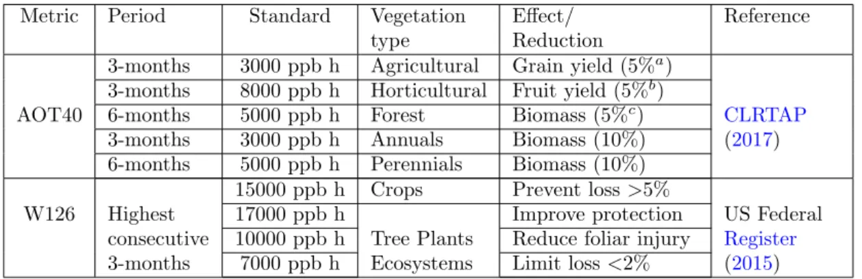
Table 1.4: Summary of ozone main standards for vegetation. (Adapted fromMills et al. (2018)).
Metric Period Standard Vegetation Effect/ Reference
type Reduction
3-months 3000 ppb h Agricultural Grain yield (5%a) 3-months 8000 ppb h Horticultural Fruit yield (5%b)
AOT40 6-months 5000 ppb h Forest Biomass (5%c) CLRTAP
(2017)
3-months 3000 ppb h Annuals Biomass (10%)
6-months 5000 ppb h Perennials Biomass (10%)
15000 ppb h Crops Prevent loss>5%
W126 Highest
consecutive 3-months
17000 ppb h Improve protection US Federal
Register (2015) 10000 ppb h Tree Plants
Ecosystems
Reduce foliar injury
7000 ppb h Limit loss<2%
aBased on wheat. bBased on tomato.
cBased on beech and birch.
is one of the most important biomass burning regions in the world. With one of the largest global deforestation rates (Artaxo et al.,2002,Malhi et al.,2008), every year, thousands of fires burn in the Amazon basin. Most fires are of anthropogenic origin, i.e., for preparation of agricultural or pastoral lands, and burn during the burning season, from July to November, across the arc of deforestation (Andreae et al.,2012) (see Figure 1.1), with dominant burning of savanna and tropical forest (94% of the fires) (Gonzalez-Alonso et al.,2019). Furthermore, the Amazon basin covers an area of about 35.5% of South America and comprises the countries of Bolivia, Brazil, Colombia, Ecuador, Guyana, Peru, Suriname and Venezuela, with a population of 25 million people (Davidson et al.,2012), including indigenous communities, unique biodiversity and a rich agriculture-based economy (i.e., cocoa, coffee, quinoa). Thus, a large portion of this population suffers regularly from high level of pollutants from biomass burning emissions (Brito et al.,2014). At the same time, the Amazon basin contains the world’s largest rainforest (Laurance et al., 2001, Aragao et al., 2014), which is a key component of the Earth System. It provides about a fifth of all of the freshwater inputs to the global oceans (Marengo and Espinoza, 2016, Nobre et al., 2016), which makes it the single, largest source of fresh water on the Earth. The Amazon rainforest stores approximately 120 billion tonnes of carbon (Malhi et al., 2006, Saatchi et al., 2011), equivalent to approximately 9—14 decades of
current global anthropogenic carbon emissions (Canadell et al., 2007), and absorbs about 1 billion tonnes of carbon per year (more than 10% of annual anthropogenic CO2 emissions) (Marengo et al., 2018). In addition, moisture exchanges in the
Amazon forest play a crucial role in the climate system, contributing to atmospheric circulation and to the water, energy and carbon cycles (Zemp et al.,2014,Spracklen and Garcia-Carreras, 2015, Nobre et al., 2016). However, climate variability and anthropogenic activities, i.e., deforestation fires, have become important agents of disturbance in the Amazon basin (Davidson et al., 2012).
Figure 1.1: Satellite image collected by the Moderate Resolution Imaging
Spectrora-diometer (MODIS) aboard the Terra satellite on August 18, 2015. Actively burning areas, detected by MODIS, are outlined in red and the arc of deforestation shaded
in red; Image adapted fromhttps://www.nasa.gov/image-feature/goddard/
el-ninos-effects-bring-more-wildfires-to-brazil.
Previous studies have sought to understand the impact of biomass burning emis-sions in the Amazon from local to hemispheric scales (Andreae et al.,1988,Kirchhoff
et al., 1989, Zhang et al., 2008, Ignotti et al., 2010, de Andrade Filho et al., 2013, Kolusu et al., 2015, de Oliveira Alves et al., 2015, Reddington et al., 2015, Archer-Nicholls et al., 2016, Martin et al., 2016, Giangrande et al., 2017). For instance, a few studies on smoke height across the Amazon have determined that smoke tends to concentrate under 2.5 km although they also found the presence of a persistent haze layer at around 4–6 km (Table1.1). These studies are based on limited obser-vations for short periods of time or specific locations, that may be influenced by specific weather conditions. Because of the lack of resources and complexities of such a complex, vast and undeveloped area, in-situ sampling in the region is scarce. Therefore, studies on biomass burning across the region have typically used satellite observations (i.e., MOPITT, MAPS and TOMS), ozonesondes and ground-based observations, combined with global and regional CTMs supplied with meteorological data and fire emission estimations. In addition, aircraft campaigns across the region have been designed to overcome the scarcity of observations, by providing with high temporal and spatial resolution data on biomass burning pollution, but limited to flight tracks. These include ABLE 2A (Harriss et al.,1988), CITE 3 (Hoell Jr et al., 1993), TRACE A (Fishman et al., 1996b), BARCA (Andreae et al., 2012), and more recently, SAMBBA (Allan et al., 2014) and GoAmazon (Martin et al., 2016). Overall, these observational and modelling studies have revealed that emissions from biomass burning in the Amazon are a large contributor to CO and O3 budgets
and their interannual variability in the southern hemisphere (SH), as well as they have shown high mixing ratios of both gases in the mid-upper troposphere over the region (e.g., Reichle et al., 1986, Andreae et al., 1988, Kirchhoff and Rasmussen, 1990, Watson et al., 1990, Fishman et al., 1996a, Galanter et al., 2000, Thompson et al., 2001, Edwards et al., 2006, Deeter et al., 2018). Substantially high surface CO and O3 mixing ratios of 400 ppb (Andreae et al., 2012) and 40—60 ppb (Bela
et al., 2015), respectively, have also been reported during the burning season, even reaching maximum daily surface O3 mixing ratios as large as 100 ppb (Artaxo et al.,
2002, Kirkman et al., 2002). The ozone levels found are well above the critical level known to be hazardous to human health and plants (40 ppb) (Ainsworth et al.,
2012). Furthermore, Pacifico et al.(2015) assessed the impact of fire-induced ozone exposure on the Amazonian tropical forest productivity and suggested enhancements of 15 ppb in O3 mixing ratios, due to biomass burning, which resulted in mean
reductions in forest productivity of 15%. Nevertheless, modelling studies across the Amazon have reported some systematic quantitative differences compared to observations, which seemed to be related to poor representation of biomass burning emissions and smoke injection heights, as well as convective and long-range transport in the models (Andreae et al.,2012, Bela et al., 2015).
Despite the large influence of biomass burning from the Amazon on the atmo-sphere budget, and the critical levels of ozone found each year during the burning season, no studies have yet comprehensively investigated the smoke plume dynamics governing the region, or assessed biomass burning impacts on surface ozone levels, with implications for human health and crops productivity. Future projections sug-gest an increase in fire activity over the Amazon region (Cochrane and Barber, 2009), exacerbated by more frequent droughts, as a consequence of climate change and human activities (Bowman et al., 2009). Under this scenario, increases of fire emissions are expected, which may lead to large, more frequent and extended epis-odes of ozone pollution, compromising larger population’s health and food security. To fully understand the factors that drive smoke plume dynamics and the transport and distribution of pollution produced in a fire is crucial to accurately predict and help mitigate impacts on air quality and climate, from local to global scales, as well as minimise the risks to human population and ecosystems.
1.2
Motivation, research objectives and approach
By 2015, an estimated area of 66% of the total Brazilian Amazonia had been de-forested (INPE, 2016). Extensive deforestation leads to changes in Amazon forest dynamics with the potential to affect the concentration of atmospheric CO2 and
roughness, stomatal resistance, soil moisture). All these changes have significant consequences on global climate, i.e., air cooling and changes in large-scale circu-lation (Nobre et al., 1991, Marengo and Nobre, 2001, Werth and Avissar, 2002). Furthermore, deforestation fires in combination with global warming and more fre-quent and severe droughts may increase biomass burning emissions and the Amazon forest may become in the near future, a source of carbon rather than a sink (Dav-idson et al., 2012).
In view of the importance of the Amazon as a global stabiliser and the large con-tribution of local biomass burning emissions to the global and regional atmospheric budget, it is crucial to have a better understanding of the drivers that control the transport and distribution of biomass burning pollution over the Amazon, its con-tribution to the atmospheric composition and its global and regional impacts. This project seeks to characterise smoke plume dynamics across the region, which will help represent the best modelling approach to study biomass burning over the Amazon, assess the contribution of biomass burning to the ground ozone levels and associa-ted impacts on air quality. For this purpose, satellite observations, ozonesondes, and aircraft and ground-based measurements combined with a global Earth System Model (ESM) are employed. Specifically, this study seeks to answer the following scientific questions:
What is the vertical distribution of biomass burning emissions over the Amazon? Determining the height at which fires inject pollutants in the atmosphere will allow understanding of how and in which degree biomass burning in the Amazon impacts the atmospheric composition, air quality and climate, from regional to global scales. Despite the importance of fire emissions from the Amazon in the global atmospheric budget, little is known about the processes that control fire pollution and plume dynamics over this region, mostly due to the lack of smoke plume height observations. This study proposes the use of a combination of satellite data during the burning seasons of 2005-2012 to develop a climatology of smoke plume heights over the Amazon. The information obtained from this analysis will help better
represent the vertical distribution of Amazonian fire emissions in ESMs.
Which are the main factors that control the vertical distribution of biomass burning emissions over the Amazon? Biomass burning in the Amazon is influenced by complex interactions among meteorology, climate, topography and human activities. Identifying main drivers of variability in fire plume dynamics across the Amazon is key to define future trends and make decisions to responsibly manage air quality and climate. On that respect, this project will evaluate the main aspects that affect smoke plume dynamics. This includes an extensive evaluation of fire properties, plume characteristics, weather and climatic conditions from 2005 to 2012.
What is the influence of biomass burning on surface O3 levels and its
impact on air quality over the Amazon? Exploring the contribution of Amazo-nian biomass burning emissions on surface ozone levels and its potential toxicity and phytotoxicity is crucial to understanding the regional and large-scale implications on air quality. For this, results from scientific questions 1 and 2 will provide information to better represent the vertical distribution of biomass burning emissions in an ESM, and assess the potential contribution of biomass burning to surface ozone levels and the impacts on air quality. This work will implement a novel fire injection height parametrisation, based on satellite observations, into an ESM and evaluate results with a combination of satellite observations, ozonesondes, aircraft and ground-based measurements. Finally, results from the modelling experiments will help widen the understanding of the impacts of fire-induced ozone on human health and vegetation across the region.
1.3
Dissertation overview
The following chapters include data, methods, analyses, results and conclusions that address the research objectives of this study. Chapter 2 presents an overview of the main features, settings, performance and limitations of the software used
to develop a climatology of smoke plumes across the Amazon for 2005-2012. This chapter addresses the first research objective. Chapter 3 presents an analysis of the climatology of smoke plume heights derived from satellite observations and assesses the main drivers of variability on smoke plume heights across the region, which directly addresses first and second research objectives. This chapter is included as a manuscript that was published on February 8th, 2019 in the Atmospheric Chemistry and Physics journal (ACP). Chapter 4 presents a modelling analysis of the impact of the vertical distribution of biomass burning on ozone and its precursors and assess the influence of Amazonian biomass burning on surface ozone and air quality over the Amazon region. This chapter is inserted as a manuscript to be submitted to ACP. Chapter 5 provides conclusions from all the analyses conducted in this work and recommendations for future research. Appendix A includes supplementary information for chapter 3. Appendix B includes supplementary information for chapter 4. Appendix C presents a summary of the chapters with contributions.
MISR and MINX: Developing a
biomass burning smoke plume
climatology across the Amazon
2.1
Introduction
Remote sensing techniques allow observing the spatial and temporal distribution of aerosols in the atmosphere, which is crucial to study their impacts on climate and air quality. Passive remote sensing techniques detect the natural radiation reflected or emitted by features under cloud-free conditions. They provide high spatial and temporal coverage, but limited accuracy on the vertical aerosols distri-bution. These passive techniques include Radiometry, Imaging Radiometry, Spec-trometry and Spectroradiometry. The latter is used by the Multi-angle Imaging SpectroRadiometer (MISR) combined with multi-image matching stereoscopic tech-niques, based on the principle of parallax (Diner et al., 1998). An important ad-vantage of this technique is that it relies uniquely on geometry and no calibration is needed, but its major limitation is its low sensitivity to thin aerosol features without a well-defined contour that is not clearly discernible from the background. On the
other hand, active remote sensing techniques send a pulse of energy and receive the radiation reflected. These techniques include Radar, Scatterometry, Laser alti-metry and LIDAR, such as the Cloud-Aerosol Lidar with Orthogonal Polarization (CALIOP), on board the CALIPSO satellite. CALIOP provides high accurate aer-osol scattering profiles (Winker et al.,2009) but extremely low spatial coverage due to its narrow path (∼60 m).
MISR and CALIOP have been widely used in the study of the vertical distribu-tion of aerosol plumes and clouds in the atmosphere over several regions (Val Martin et al., 2010, Amiridis et al., 2010, Jian and Fu, 2014, Huang et al., 2015). For ins-tance, over North America, Val Martin et al. (2010) developed an extensive 5-year climatology of smoke plume heights based on height-retrievals derived using MISR imagery. Similarly, Jian and Fu (2014) and Tosca et al. (2011) characterised smoke plume heights during the burning seasons of 2001–2009/2010, over tropical regions in Asia and Mims et al. (2010), over grassland fires in Australia. Using observa-tions made by CALIOP, Huang et al. (2015) examined the most probable height of dust and smoke layers over six fire impacted regions and Amiridis et al. (2010) investigated aerosols vertical distribution and smoke top heights from agricultural burning in Europe. All these studies showed the large variability in smoke plumes across biome, season and region, as well as demonstrated that although most smoke concentrates in the boundary layer, where it is well-mixed, a variable but significant percentage of generally, low-density smoke reaches the free troposphere, as a result of favourable fire and local weather conditions, and can be transported long-range distances. MISR and CALIOP performance and sensitivity are disparate. Speci-fically MISR provides near-source constraints on the vertical distribution of smoke and allows to study smoke plume dynamics on a plume-by-plume case.
The Amazon region is a major fire region, which contributes largely to the global fire emissions (Van der Werf et al., 2010). However, despite its important role in the distribution and transport of global biomass burning products, no study has yet developed a climatology of smoke plume heights over the region. The present study
aims at improving the vertical distribution of biomass burning emissions represented in Earth system models (ESM) over the Amazon. For that, MISR capabilities are exploited to develop a large dataset of smoke plume heights during the burning seasons (July to November) from 2005–2012. This is the first time that such a comprehensive study of the vertical distribution of biomass burning emissions has ever been done over the Amazon. The smoke plume database developed over the Amazon presented in Chapter 3 (Gonzalez-Alonso et al., 2019) was created with the MINX interactive tool (Nelson et al., 2008b, 2013), using the MISR imagery and MODIS thermal anomalies (Diner et al.,1998,Giglio et al.,2003). Because the use of MINX requires some understanding of the software and algorithms used, this chapter describes the principal features of the MISR instrument and performance of MINX, with focus on the Amazon smoke plume climatology.
2.2
MISR Instrument and products
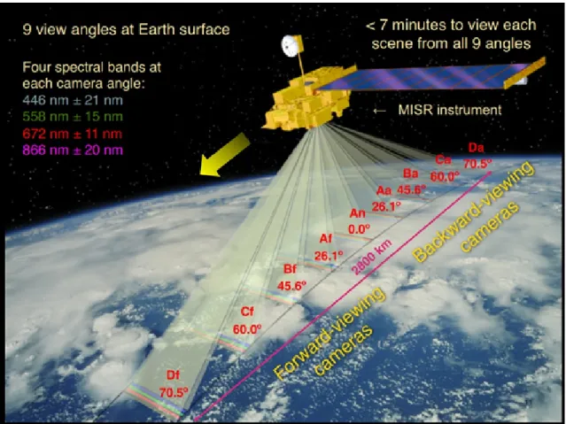
The Multi-angle Imaging SpectroRadiometer (MISR) is a spaceborne instrument that measures atmospheric and surface properties, designed to study cloud, aerosols and the Earth surface. MISR flies on board the Terra satellite (launched in December 1999) and since February 2000 has been acquiring images of the Earth at nine different fixed angles (from -70°to 70°)(Diner et al.,1998). This multi-angle imagery provides stereoscopic retrievals of aerosol plumes and clouds heights at 275 m to 1.1 km of resolution. MISR is integrated in the NASA Earth Observing System (EOS) fleet, with a near-polar orbit at an altitude of 705 km and about 380 km of swath common to all cameras. The descending node crosses the Equator at around 10:30 a.m. local time and provides global coverage every 9 days at the equator and every two days near the poles.
The nine push-broom cameras are designated as An, for the nadir camera and A, B, C and D followed by ”a” or ”f” , depending of their viewing, being ”a” for aft-viewing and ”f” for forward-viewing (i.e., Aa, Ba, Ca, Da and Af, Bf ,Cf Df;
Figure 2.1). The camera viewing angles differ in approximately 7 min from each other and 70.5°(D), 60.0°(C), 45.6°(B), and 26.1°(A) from the nadir. Images are ac-quired in four spectral channels for each camera at blue, green, red and near-infrared wavelengths (446.4±41.9; 557.5±28.6; 671.7±21.9 and 866.4±39.7 nm, respectively). More information about the MISR instrument can be found in Diner et al. (1998) and at https://misr.jpl.nasa.gov/Mission/misrInstrument/.
Figure 2.1: TERRA satellite with MISR aboard, and the four-spectral-band multi-angle nine
cameras;https://github.com/nasa/MINX/blob/master/webdoc/MINX_Doc1.pdf.
MISR data are freely downloadable from the Earth Data website1, following registration and logging in. Data include three level products and ancillary data. The Levels 1 and 2 products are in swaths of 180 blocks of 140.8 km along track for each MISR orbit. Level 1 products have been processed and calibrated radio-metrically and georadio-metrically to remove many of the instrument effects. Level 2
1
products are geophysical measurements derived from the instrument data. They include Level 2 Top-of-Atmosphere/Cloud product, with cloud heights and winds, cloud texture, top-of-atmosphere albedos and other related parameters, and Level 2 Aerosol/Surface product, with tropospheric aerosol optical depth, aerosol com-position and size, among other parameters. Level 3 product consists of monthly, seasonally, and annually averaged maps for various parameters from Level 2. The NASA Langley Atmospheric Science Data Center2 distributes the MISR products in hierarchical data format (HDF). Detailed description of the algorithms used for each data product and specifications of the HDF files can be found in the Atmospheric Science Data Center (ASDC) website3.
The stereo-matching algorithms in the operational MISR Level 2 cloud product use MISR multi-angle ellipsoid-referenced images to automatically retrieve heights and winds of clouds, and other aerosol features above the ground using a stereoscopic method (Moroney et al., 2002a). For that, MISR needs a previous set of some fixed processing parameters, which will be applied equally to all scenes (Muller et al., 2002) to speed-up processing time. If all cameras measured high-resolution radiances, MISR data would be prohibitive. For this reason, only the nadir camera data and the red channels for the off-nadir cameras (12 of the 36 channels) are kept at the highest resolution (275 m), while data on the other channels are at 1.1 km resolution. This operational mode is the default and is called global mode (GM), useful for global studies of cloud heights and winds. However, MISR can also be configured to achieve high resolution for all the channels (36 channels) for a limited period of time and specific domains. This capability is known as the local mode (LM) and it is scheduled upon request from the user community.
The MISR operational product retrieves two types of stereo-heights. The zero-wind heights assume that disparity in the same feature between camera views is
2
https://eosweb.larc.nasa.gov/; last access 10/02/2019
3
https://eosweb.larc.nasa.gov/sites/default/files/project/misr/guide/MISR_
Science_Data_Product_Guide.pdf; https://eosweb.larc.nasa.gov/project/misr/misr_
caused by parallax. Parallax is the difference in location of a projected feature on the ground due to different viewing angles (Moroney et al., 2002a). Smallest par-allax is obtained from the nadir image (An) and is used as the reference camera. Wind-corrected heights are calculated after separating the contribution of the wind and the parallax to that disparity. They need the wind speed along-track and across-track components to be computed and applied to the zero-wind cloud-top heights to produce wind-corrected heights at a horizontal resolution of 1.1 km. The wind direc-tion and the along-track component of the wind speed are extracted using the Df/Da (±70°) and Bf/Ba (±46°) cameras imagery (Davies et al., 2007). Wind-corrected heights provide more accurate results, but are computationally expensive and at low spatial coverage, unlike the zero-wind heights, which offer excellent coverage (Kahn et al., 2007).
2.3
MODIS Instrument and products
The MODIS instrument is also aboard the NASA Terra satellite and observes the same scenes as MISR. MODIS detects from its far-infrared imagery, under cloud-free conditions, thermal anomalies at 1 km spatial resolution, named ”fire pixels”, (Figure 2.2). The detection method is based on an algorithm (Giglio et al., 2003) that exploits the strong emission of mid-infrared radiation from fires (Dozier, 1981, Matson and Dozier, 1981) and offers automated daily global fire information. In addition, MODIS provides estimates of the fire radiative power (FRP) for each fire pixel detected, a parameter used as a proxy of fire intensity. FRP is calculated from the differences in the radiance of each fire pixel and its background (Giglio et al., 2003). Two MODIS products are assimilated by MINX:
1. The Level 2 MOD14 Thermal Anomalies at a 1 km resolution, which includes FRP.
the MODIS Level 3 land cover product MCD12Q1 Land Cover Product4 (Friedl et al., 2010). This MCD12Q1 product classifies the land cover asso-ciated with each smoke plume in 17 International Geosphere-Biosphere Pro-gramme (IGBP) land cover classes and has an annual temporal resolution.
Figure 2.2: Natural-colour image collected by the Terra satellite across the
Amazon on September 10, 2015. Actively burning areas, detected by MODIS’s
thermal bands, in red. https://www.nasa.gov/image-feature/goddard/
wildfires-in-amazonian-region-of-brazil.
2.4
MINX Software
The MINX visualization and analysis interactive tool complements the MISR Level 2 operational stereo product for detailed studies of smoke, dust and volcanic ash.
The MINX stereo-height algorithm was developed to overcome the limitations of the MISR operational product, as it enables the user to retrieve clouds, aerosols plume heights and winds at higher spatial resolution and better precision. Plumes are defined as regions of dense aerosol, with a well-defined discernible contour above the terrain and downwind of its source (Nelson et al., 2013), allowing to determine the direction of transport. Clouds, on the other hand, are not associated with any source and the direction of transport is not evident. MINX is written in the Interactive Data Language (IDL) and it can be downloaded from Github5, available for Mac OS X, MS Windows, and Linux platforms. Since the development of MINX, several versions have been released. The latest version is MINXv4, with substantial improvements that provide better quality smoke height retrievals. MINX has been used for the MISR Plume Height Climatology Projects (MPHCP)6. MPHCP aims at creating an aerosol injection height climatology to support wildfire, climate change, and air quality studies (Nelson et al., 2008b). In addition, MINX uses have been extended to many detailed studies of smoke plume heights over specific regions in the world (Val Martin et al., 2010,Mims et al., 2010, Tosca et al., 2011), studies of ash clouds from volcanic eruptions (Scollo et al., 2012,Kahn and Limbacher, 2012) and dust plumes from deserts (Kalashnikova and Kahn, 2008).
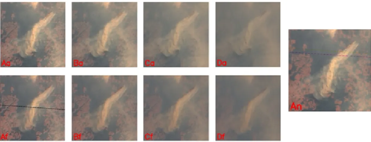
MINX interface allows the user to display the multi-angle nine camera images one by one or as an animated loop (Figure 2.3). This method enables the user to study plume and cloud dynamics, as it provides a similar 3D effect of the scene that could not be possible with a single image or multiple same-angle images. MINX requires all nine camera terrain-referenced imagery files (GRP TERRAIN product) to derive accurate heights and winds over land (Jovanovic et al., 1998), and the geometric parameters product (GP GMP), with zenith and azimuth viewing angles, which are both from MISR Level 1. An additional product is needed to perform stereo retrievals, the MISR Ancillary Geographic Product (AGP) at 1.1 km spatial
5https://github.com/nasa/MINX; last access 12/02/2019
6https://misr.jpl.nasa.gov/getData/accessData/MisrMinxPlumes2/; last access
resolution, which contains the Digital Elevation Model (DEM) and surface feature IDs. Additionally, MISR Level 2 aerosol parameters (AS AEROSOL) are used to obtain aerosol data, i.e., AOD, and TC CLASSIFIERS to identify different types of aerosols (e.g., smoke or ash). All the cited products can be downloaded from the Earth data website7 after logging in. Table 2.1 summarises the MISR and MODIS products and files necessary to process smoke plume heights with MINX.
Figure 2.3: MISR nine camera views of a smoke plume on the 22nd of August 2010, in the
Amazon
As the MISR operational product, MINX stereo-height algorithm provides zero-wind and zero-wind-corrected height values (Figure 2.4). MINX calculates the wind speed necessary to retrieve wind-corrected plume heights with an accuracy of 250 m by supplying the wind direction in the plume. For each grid in a plume, heights and winds are computed combining each of the six nearest camera neighbours to the nadir camera, used as a reference. Whenever the results of at least three camera pairs are similar, the retrieval is considered successful. In addition, if the MISR aerosol standard products are loaded in MINX, aerosol properties within the plume (e.g. Angstrom exponent, single-scattering albedo) will be extracted at 17.6 km of resolution.
T able 2.1: Summa ry of MISR and MODIS files and p ro ducts used to digitise smok e plumes with MINX. Pro duct Files Description MODIS MOD14 a MODIS/T erra Thermal Anomalies/Fire 5-Min L2 Sw ath 1km V005 fire pixels at 1 km and FRP in MW/pixel MI1B2T b lev el 1 GRP TERRAIN (terrain-referenced) radiance files MIB2GEOP b lev el 1 GP GMP camera and sun geometry MIANCA GP b A GP – ancillary geographic digital elev ation data and su rface typ e masks MIL2ASAE c lev el 2 AS AER OSOL aerosol data: A OD, single-scatter alb edo etc. MIL2TCCL a lev el 2 TC CLASSIFIERS smok e/cloud mask files a Optional files b Required files c Required only for plume studies
2.4.1
MINX Stereo retrieval algorithm
The retrieval process starts by matching images of camera pairs with the nadir camera and measuring the disparities within a plume. When the user determines the wind direction for each camera pair a height, wind-across-track and wind-along-track solution is achieved. This process is done for all camera pairs at the same point, and a maximum of eight heights and wind values are obtained depending on the number of camera pairs selected for matching and the number of successful retrievals. Then, the MINX stereo retrieval algorithm determines the more similar height and wind value among camera pairs for each point.
Height retrievals for static and in movement features
During Terra overpass, each MISR camera observes a feature in the atmosphere within seven-minute difference. The shift in the location of a feature between two cameras is its disparity, and consists of an along-track displacement parallel to the ground, and an across-track displacement in the orthogonal direction. The
measure-Figure 2.4: Comparison of wind-corrected and zero-wind stereo-height pixels per plume in a
ments of these two components provide the primary information to compute stereo heights and winds (Moroney et al., 2002a).
In the case of static features in the atmosphere, the along and across-track dis-parities due to motion are zero, the across-track disparity due to parallax is zero and the along-track disparity is only due to parallax. Therefore, its height can be determined by knowing this parallax disparity and the angle of the non-nadir cam-era (Moroney et al., 2002b)(Figure 2.5). This is called the zero-wind height. The zero-wind height can also be performed for features in movement however, errors range from tens of meters to kilometres, depending on the height of the feature, the wind and the camera pair used.
If the feature is not stationary, then the height, the wind speed in the along- and across-track directions are unknown for a camera pair, assuming no vertical motion. In the MISR operational product this is solved by adding a third camera pair (D) and making some assumptions (Zong et al., 2002) (Section 2.2). In MINX, there are two cases to perform the stereo height retrieval. The case in which the feature moves only in the across-track wind component and the case in which the feature moves in both components, along and across-track. In the first case, the along-track disparity due to motion is zero and the height is determined in the same way as the zero-wind height performance, assuming that the along-track disparity is only due to parallax. The across-track wind speed can then be determined by converting the across-track disparity to map distance and dividing by the time between the two camera viewing angles. To compute this height the Earth’s curvature, terrain height and other factors need to be considered. When a feature is moving in the two components, the across-track wind component will be determined using the method described above but the along-track component includes the contribution of the parallax and the real displacement due to the along-track wind. In this case, the height and the along-track wind components need to be determined, knowing only the along-track disparity.
Figure 2.5: MISR view with respect to features in the atmosphere, disparities produced by parallax and due to motion of the MISR instrument and the feature. (Image adapted from
https://github.com/nasa/MINX/blob/master/webdoc/MINX_Doc5.pdf).
direction when digitising (Section 2.4.2). For any point in the user-supplied wind direction, the wind direction can be calculated as the slope of the digitised line, which is the ratio of the along- and across-track distances and the ratio of the wind speed in the along- and across-track components. If one of the wind speeds is known, the other can be calculated from the slope of the line and the along-track wind, and height can be determined at high resolution using a camera pair. This stereo retrieval method is applied to each point of the digitised plume using all camera pairs and the nadir camera as reference.
Image matching
The image matching process consists of finding a feature in a non-nadir image that corresponds to that feature in the nadir image and measuring its disparity. During the MINX stereo height retrievals, all cameras selected for image matching should be paired with the nadir camera. Meaning that whenever a feature is not visible
in the nadir camera but visible in any of the off-nadir cameras, MINX will fail at performing the stereo retrieval. This process uses a square template-based reference image in the red-band, centred on the pixel of study in the nadir view. The match is performed when a target pixel in the comparison image is found to best correlate to the reference template. This method provides more accurate matcher results applied to features that extend through the template than to a single pixel at the centre. The image matching process requires intense use of the CPU, and processing times depend on the hardware and the area to perform the match. Larger templates require longer processing times and can improve the retrieval coverage, but the smaller are usually more successful for fine spatial detail when plumes have small variations in height. The matcher template size is defined by the user. In the case of the Amazon climatology of smoke plumes, the default option (medium size) was chosen, which provides enough detail at reasonable processing times.
Determination of height and wind
Once the successful matches for the camera pairs produce the retrieved results for a sample point, these results are then evaluated to determine a consensus height and wind for all camera pairs matching. The mean heights and winds are calculated for those camera pairs retrievals that are more similar to the median values, used to soften the effects of the outliers. Heights and wind results are discarded if they do not fall into a threshold distance from the media, where the threshold distances are calculated dynamically.
Spectral band
The red band is the high-resolution band in the global mode of the MISR operational product because of its larger contrast between atmospheric features over ocean and land (Diner et al., 1998). However, over bright surfaces like grasslands or deserts, or in the case of low-dense features stereo-height retrievals in red band is not
pre-ferred (Mims et al.,2010). Increases in wavelength lead to decreases on atmospheric scattering and smoke will be more transparent, allowing to see the terrain through it. If in the reference image the terrain is seen through the smoke plume, the image matching will be more difficult to process, performing less successful height retriev-als. Therefore, blue band retrievals generally offer greater sensitivity to thin aerosol layers and over bright surfaces.
Before the release of MINXv4 the default spectral band option was red. However, the user could select the blue band if applicable to the characteristics of the plume and background. This should be configured by the user manually at the start of digitising each plume, which entails additional time into the digitising process. Since MINXv4, two plume height retrievals are performed for each plume. One retrieval using red-band data and the other using blue-band data. Each retrieval is treated as a different plume, but they share the same aerosol properties, from the MISR aerosol product, and the same plume coded name in exception of a letter, ”R” or ”B”, depending on the spectral band (”R” for red and ”B” for blue band). This new capability allows the user to choose between the best quality height retrieval plume, but it doubles the number of plumes created.
2.4.2
Digitalization of smoke plumes with MINX
MINX can be used to digitise and study a single plume or to create a large clima-tology of smoke plumes observed by MISR. The files generated by MINX include among other parameters the location and time of the plume, different statistics for smoke plume heights based on the individual height retrievals, the radiative power of the associated fires, the direction of transport of plumes and aerosol properties.
MISR files are large (∼2 Gbytes/orbit) and tedious to download for projects that cover large periods of time or areas, like this study. The MINX ”Plume Utilities” is a tool designed to limit the amount of MISR data to download and process, reducing considerably processing time and computing space. This tool allows the user to
select only the MISR orbits and blocks where it is likely to find smoke plumes, rather than download and visually inspect all MISR images for the time range and area of study. In the case of smoke plumes from wildfires, MINX uses the MODIS Terra thermal anomalies product, as mentioned in Section 2.3. By loading the fire pixels, MINX generates a list of the MISR orbits and blocks with coincident active fire pixels. To do so, the user needs to provide the geographic bounds and the time range for the study when ordering the MODIS MOD14 thermal anomalies. The ”Plume Utilities” tool reduces the number of MISR files to download by a factor of 100 or more (Nelson et al.,2008b). In addition, the MODIS thermal anomalies files are read by MINX and displayed as a layer of red dots on MISR imagery (Figure2.2), which helps the user identify plumes, and allows MINX to compute the approximate total FRP for each plume.
Once the necessary MODIS fire pixels and MISR Level 1 and 2 files are down-loaded (Table 2.1), MINX is ready to process them, display and compute stereo heights of smoke plumes. Before digitising, the user needs to load and link the MODIS fire pixels to the MISR orbits and paths images. This step includes spe-cifying some parameters as the minimum number of fire pixels to consider or their confidence level. For the specific case of the Amazon climatology, the default op-tions were selected as presented in Figure 2.6. Following this, MINX loads the MODIS thermal anomalies on the MISR images (Figure 2.2). At this point, the user inspects the MISR multi-imagery block by block with the coincident fire pixels superimposed and identifies smoke plumes. The ability to visualise each plume in nearly 3D is decisive to study its structure and dynamics.
The digitising process starts by drawing with the mouse the contour of the plume, starting at the fire source, and the direction of transport. Plumes direction can be digitised with as many points as necessary, being common to draw only two points in the case of a quite linear plume. It is important to make sure that all fire pixels associated with the same plume are contained within the digitised area, as MINX computes the total FRP for each plume and if any fire pixel is not included, it