Adaptive Sliding Mode Observer for Nonlinear Interconnected Systems with Time Varying Parameters

(1)

Kent Academic Repository

Full text document (pdf)

Copyright & reuse

Content in the Kent Academic Repository is made available for research purposes. Unless otherwise stated all content is protected by copyright and in the absence of an open licence (eg Creative Commons), permissions for further reuse of content should be sought from the publisher, author or other copyright holder.

Versions of research

The version in the Kent Academic Repository may differ from the final published version.

Users are advised to check http://kar.kent.ac.uk for the status of the paper. Users should always cite the published version of record.

Enquiries

For any further enquiries regarding the licence status of this document, please contact:

[email protected]

If you believe this document infringes copyright then please contact the KAR admin team with the take-down information provided at http://kar.kent.ac.uk/contact.html

Citation for published version

Mohamed, Mokhtar and Yan, Xinggang and Mao, Zehui and Jiang, Bin (2018) Adaptive Sliding

Mode Observer for Nonlinear Interconnected Systems with Time Varying Parameters. Asian

Journal of Control . (In press)

DOI

Link to record in KAR

http://kar.kent.ac.uk/69232/

Document Version

Author's Accepted Manuscript

(2)

Asian Journal of Control, Vol. 00, No. 0, pp.1–10, Month 2008

Published online in Wiley InterScience (www.interscience.wiley.com) DOI: 10.1002/asjc.0000

Adaptive Sliding Mode Observer for Nonlinear Interconnected Systems

with Time Varying Parameters

⋆

Mokhtar Mohamed, Xing-Gang Yan, Zehui Mao, and Bin Jiang ABSTRACT

In this paper, a class of nonlinear interconnected systems with uncertain time varying parameters (TVPs) is considered. Both the interconnections and the isolated subsystems are nonlinear. Sliding mode control method and adaptive techniques are employed together to design an observer to estimate the state variables of the systems in presence of unknown TVPs. The Lyapunov direct method is used to analysis the stability of the sliding motion and it is not required to solve the so-called constrained Lyapunov problem (CLP). A set of conditions is developed under which the augmented systems formed by the error dynamical systems and the designed adaptive laws, are globally uniformly ultimately bounded. A simulation example is presented and the results show that the method proposed in this paper is effective.

Key Words: Sliding Mode Observer, Nonlinear Interconnected Systems, Adaptive Techniques, Time Varying Parameters

I. INTRODUCTION

In the modern world, it is required to deal with advanced systems using advanced technologies, which has resulted in many large-scale complex systems. With the increasing requirement for the system performance, it needs to develop novel techniques to achieve novel design to satisfy the requirements. It should be noted that control design for large-scale interconnected systems has obtained great achievement [1,2]. However, lots of results are based on the fact that all system state variables are available for design, which does not always hold and actually only partial state variables are usually available in reality [1]. Therefore,

Mokhtar Mohamed and Xing-Gang Yan are with the School of Engineering and Digital Arts, University of Kent, Canterbury, Kent CT2 7NT, United Kingdom (Emails: [email protected]; [email protected]).

Zehui Mao and Bin Jiang are with the College of Automation Engineering, Nanjing University of Aeronautics and Astronautics, Nanjing, 211106, P. R. China (Emails: [email protected]; [email protected]).

∗_{The authors gratefully acknowledge the support of the}

National Natural Science Foundation of China (61573180) for this work.

observer design is one of the main topics to estimate system states using the available system inputs and outputs in control engineering.

The concept of the observer was first introduced by Luenberger in 1964 where the observation error between the output of the actual plant and the output of the observer converges to zero when time goes to infinity. Subsequently, many approaches have been developed to design observers for different systems to estimate system states (see e.g. [3,4,5,6]). However, the problem becomes more challenging when some parameters in the model of the system are unknown, particularly when these parameters are time varying [7]. Over the last few decades, much literature has been devoted to the design of adaptive observers for linear and nonlinear systems. The early results are mainly for linear systems (see e.g. [8] and references therein). Later, many authors have focused on the development of adaptive observer design for nonlinear systems (see e.g. [9, 10]). In these results, the designed adaptive observers are able to maintain bounded parameters estimation error under the persistence of excitation condition and it is required that the unknown parameters are bounded with some extra constraints imposed on the system.

c

2008 John Wiley and Sons Asia Pte Ltd and Chinese Automatic Control Society Prepared usingasjcauth.cls[Version: 2008/07/07 v1.00]

(3)

More recently, adaptive observers using different

techniques have been proposed in (see e.g. [11,

12]) where the unknown parameters are limited to

be constant. Compared with much existing work in adaptive observer design with unknown constant parameters, the corresponding observation results for unknown time varying parameters (TVPs) are very limited. The approach for nonlinear time varying

systems proposed in [13] is based on the fact

that the nonlinear systems can be transformed to a particular observable canonical form, and the unknown parameters are bounded. The authors in [14] proposed a sampled output high gain observer for a class of uniformly observable nonlinear systems where the unknown parameters are bounded. An adaptive estimator is proposed in [15] to estimate TVPs for nonlinear systems. However, all the system states are assumed available. In [16] an adaptive observer for a class of nonlinear interconnected systems with uncertain TVPs has been developed. It is required to solve the well known constrained Lyapunov problem (CLP) (see e.g. [17,18]). The authors in [19] used an adaptive unscented Kalman filter approach to estimate the time varying parameters and system states of a class of nonlinear high-speed objects. This technique requires the assumption that the additive noise vectors are Gaussian uncorrelated white noises. If the assumption is not satisfied, the estimation process accuracy will be significantly affected [20].

Sliding mode techniques have been successfully used in control design and state estimation due to its attractive features such as high robustness to uncertainties in input channel and to parameters variations (see e.g. [21, 22]). An adaptive observer applying sliding mode techniques have been developed in [23] to enhance the performance of the adaptive

observer proposed by [24]. Adaptive sliding mode

observer based fault reconstruction for nonlinear systems with parametric uncertainties is considered in [25]. However, the unknown parameters considered in these papers are constant. Many adaptive observers have been developed using sliding mode techniques for particular applications and for particular purposes (see e.g. [26,27]) and thus corresponding specific conditions need to be imposed on the systems considered. Sliding mode techniques with super twisting algorithm are used in [28] to design adaptive observers for nonlinear systems where the unknown parameter vector is assumed to be constant. Sliding mode synchronization method is combined with adaptive techniques in [29] to estimate the unknown parameters for multiple chaotic systems where the system states are assumed to be

known and the unknown parameters are constant. To the best of authors’ knowledge, this is the first contribution where sliding mode techniques are applied to design an adaptive observer for nonlinear interconnected systems with unknown TVPs.

In this paper, an adaptive sliding mode observer is established for a class of nonlinear interconnected systems with unknown TVPs, in which both the isolated subsystems and interconnections are nonlinear. It is not required that the bounds on the TVPs are known, but the rate of change of these unknown parameters needs to be bounded. Sliding mode techniques and adaptive techniques are employed together to estimate system states with unknown TVPs. In addition, it is not required to solve the CLP. Sufficient conditions are developed such that the augmented systems formed by the error dynamical system and the designed adaptive laws, are globally uniformly ultimately bounded. Simulation results for a numerical nonlinear interconnected system are presented to demonstrate the effectiveness of the developed results.

II. System Description and Preliminaries

Consider a nonlinear interconnected system com-posed ofNsubsystems as follows

˙ xi =Aixi+gi(xi, ui)+φi(yi, ui)Θi(t) + N X j=1 j6=i Hij(xj) (1) yi =Cixi (2)

where xi∈Ωi⊂Rni (Ωi are neighborhoods of the

origin),ui∈Ui∈Rmi (Ui are the admissible control

sets) and yi∈Rpi with mi≤ pi≤ni are the state

variables, inputs and outputs of the i-th subsystem respectively, gi(xi, ui)∈Rni are nonlinear known

functions, φi(yi, ui)∈Rni are known functions and

Θi(t)∈R are unknown TVPs. The matrix triples

(Ai, Ci)are constant with appropriate dimensions and

Ci are full row rank. The terms PNj=1

j6=iHij(xj)are the

known interconnections fori= 1,· · ·, N.

Since the Ci are full row rank, there exist

nonsingular matricesTci such that

¯ Ai = _¯ Ai1 A¯i2 ¯ Ai3 A¯i4 :=TciAiT −1 ci , (3) ¯ Ci = 0 Ipi :=CiTc−i1 (4)

whereA¯i1∈R(ni−pi)×(ni−pi) fori= 1,· · ·, N. Then

in the new coordinatesx¯idefined by

c

(4)

3

¯

xi=Tcixi (5)

system (1)-(2) can be rewritten as ˙¯ xi1 = A¯i1x¯i1+ ¯Ai2x¯i2+ ¯gi1(¯xi, ui) + ¯φi1(yi, ui)Θi(t) + N X j=1 j6=i H_ija(¯xj) (6) ˙¯ xi2 = A¯i3x¯i1+ ¯Ai4x¯i2+ ¯gi2(¯xi, ui) + ¯φi2(yi, ui)Θi(t) + N X j=1 j6=i H_ijb(¯xj) (7) yi = x¯i2 (8)

where x¯=col(¯x1,x¯2,· · · ,x¯N), x¯i=col(¯xi1,x¯i2),

¯ xi1∈Rni−pi, x¯i2∈Rpi, and ¯ gi1(¯xi, ui) ¯ gi2(¯xi, ui) : = ¯gi(¯xi, ui)=Tci[gi(xi, ui)]xi=Tci−1x¯i(9) _¯ φi1(yi, ui) ¯ φi2(yi, ui) : =Tciφi(yi, ui), (10) Ha ij(xj) Hb ij(xj) : =Tci[Hij(xj)]xj=Tcj−1x¯j (11)

Assumption 1.The uncertain TVPsΘi(t)satisfy

|Θ˙i(t)| ≤µi (12)

whereµiare known constants andµi >0.

Assumption 1 means the bounds on the unknown TVPs are not required, but the rate of changes of these parameters are required to be bounded.

Assumption 2.The matrix pairs( ¯Ai,C¯i)in (3)-(4) are

observable fori= 1,2,· · · , N.

Under Assumption 2, there exist matricesLi such

thatA¯i−LiC¯i are stable, and thus for anyQi>0the

Lyapunov equations

( ¯Ai−LiC¯i)TPi+Pi( ¯Ai−LiC¯i) =−Qi (13)

have unique solutionsPi>0fori= 1,2,· · · , N.

For further analysis, introduce partitions ofPiand

Qi which are conformable with the decomposition in

(6)-(8) as follows Pi= Pi1 Pi2 PT i2 Pi3 , Qi= Qi1 Qi2 QT i2 Qi3 (14) wherePi1∈R(ni−pi)×(ni−pi), Qi1∈R(ni−pi)×(ni−pi).

Then, fromPi >0andQi>0, it follows thatPi1>0,

Pi3>0,Qi1>0 andQi3>0. The following result is

required for further analysis.

Lemma 1.The matricesA¯i1+P_i−11Pi2A¯i3are Hurwitz

stable, wherePi1 andPi2 are defined in (14) andA¯i1

andA¯i3 are defined in (3), if the Lyapunov equations

(13) are satisfied.

Proof.See Lemma 2.1 in [30].

Assumption 3. The functions¯gi(¯xi, ui)defined in (9)

satisfy the Lipschitz condition with respect tox¯i∈Rni

and uniformly forui ∈Ui∈Rmi fori= 1,2,· · ·, N.

Assumption 3 implies that there exist nonnegative functionsℓ¯gi1andℓg¯i2 such that

k¯gi1(¯xi, ui)−¯gi1(ˆx¯i, ui)k ≤ ℓg¯i1(ui)kx¯i−xˆ¯ik(15)

k¯gi2(¯xi, ui)−¯gi2(ˆx¯i, ui)k ≤ ℓg¯i2(ui)kx¯i−xˆ¯ik(16)

fori= 1,2,· · ·, N.

Remark 1. Assumption 3 shows that the functions ¯

gi(¯xi, ui)defined in (9) satisfy the Lipschitz condition

with respect to only x¯i instead of (¯xi, ui). Such an

Assumption is reasonable because control inputsuiare

usually known in observer design, and may relax the limitation to the functions¯gi(¯xi, ui).

III. Adaptive Sliding Mode Observer Design

Consider the system in (6)-(8). Introduce a linear coordinate transformation zi= Ini−pi Ki 0 Ipi | {z } Ti ¯ xi (17)

whereKi=Pi−11Pi2. In the new coordinate systemzi,

system (6)-(8) has the following form ˙ zi1 = ( ¯Ai1+KiA¯i3)zi1+ ( ¯Ai2−A¯i1Ki+Ki( ¯Ai4 −A¯i3Ki)zi2+ ¯gi1(Ti−1zi, ui) + ¯φi1(·)Θi(t) +Kig¯i2(Ti−1zi, ui) + N X j=1 j6=i H_ija(T−1z) +Kiφ¯i2(yi, ui)Θi(t) +Ki N X j=1 j6=i Hijb(T−1z)(18) ˙ zi2 = ¯Ai3zi1+ ( ¯Ai4−A¯i3Ki)zi2+ ¯gi2(Ti−1zi, ui) + ¯φi2(·)Θi(t) + N X j=1 j6=i H_ijb(T−1z) (19) yi = zi2 (20)

wherezi=col(zi1, zi2)withzi1∈Rni−pi. For system

(18)-(20), consider a dynamical system

c

2008 John Wiley and Sons Asia Pte Ltd and Chinese Automatic Control Society Prepared usingasjcauth.cls

(5)

˙ˆ zi1 = ( ¯Ai1+KiA¯i3)ˆzi1+ ( ¯Ai2−A¯i1Ki+Ki( ¯Ai4 −A¯i3Ki))yi+ ¯gi1(T_i−1zî, ui) + ¯φi1(·) ˆΘi(t) + N X j=1 j6=i H_ija(T−1zˆ) +Kig¯i2(T_i−1zî, ui) +Kiφ¯i2(·) ˆΘi(t) +Ki N X j=1 j6=i H_ijb(T−1zˆ) (21) ˙ˆ zi2 = ¯Ai3zî1+ ( ¯Ai4−A¯i3Ki)yi+ ¯gi2(Ti−1zî, ui) + ¯φi2(·) ˆΘi(t) + N X j=1 j6=i H_ijb(T−1zˆ) +di(·) (22) ˆ yi = ˆzi2 (23)

where zˆ=col(ˆz1, y), and the injection term di(·) is

defined by

di(·) = ρisgn(yi−yˆi) (24)

whereρiare positive constants fori= 1,2,· · ·, N, with

adaptive laws

˙Γi = −σi[ ˙ˆyi−di(·)] (25)

ˆ

Θi(t) = Γi+σiyi (26)

where di(·) is given in (24), and σi are positive

constants. Letei1=zi1−ˆzi1,eyi=yi−yˆi andeΘi =

Θi(t)−Θˆi(t). Then from (18)-(20) and (21)-(23), the

error dynamics are described by ˙ ei1= ( ¯Ai1+KiA¯i3)ei1+ [¯gi1(·)−g¯i1(ˆ·)]+¯φi1(·)[Θi(t) −Θî(t)]+ N X j=1 j6=i [H_ija(·)−H_ija(ˆ·)]+Ki[¯gi2(·)−¯gi2(ˆ·)] +Kiφ¯i2(·)[Θi(t)−Θî(t)]+Ki N X j=1 j6=i [H_ijb(·)−H_ijb(ˆ·)](27) ˙ eyi= ¯Ai3ei1+ [¯gi2(·)−g¯i2(ˆ·)] + ¯φi2(·)[Θi(t)−Θî(t)] + N X j=1 j6=i [H_ijb(·)−H_ijb(ˆ·)]−di(·) (28)

wheredi(·)is given in (24) fori= 1,2,· · ·, N, and

¯ gi1(Ti−1zi, ui) = ¯gi1(·), ¯gi1(Ti−1ˆzi, ui) = ¯gi1(ˆ·) ¯ gi2(T_i−1zi, ui) = ¯gi2(·), ¯gi2(T_i−1ˆzi, ui) = ¯gi2(ˆ·) Ha ij(T−1z) = Hija(·), Hija(T−1zˆ) =Hija(ˆ·) H_ijb(T−1z) = H_ijb(·), H_ijb(T−1zˆ) =H_ijb(ˆ·) From (25) and (26) ˙ eΘi = Θ˙i(t)−Θ˙ˆi(t) = ˙Θi(t)− {˙Γi+σiy˙i} = Θ˙i(t)− {−σi[ ¯Ai3zˆi1+ ( ¯Ai4−A¯i3Ki)yi +¯gi2(ˆ·) + ¯φi2(·) ˆΘi(t) + N X j=1 j6=i H_ijb(ˆ·) +di(·) −di(·)]}+{σi[ ¯Ai3zi1+ ( ¯Ai4−A¯i3Ki)zi2 +¯gi2(·) + ¯φi2(·)Θi(t) + N X j=1 j6=i H_ijb(·)]} = −σiA¯i3ei1−σi[¯gi2(·)−g¯i2(ˆ·)]−σiφ¯i2(·)eΘi − N X j=1 j6=i σi[Hijb(·)−Hijb(ˆ·)] + ˙Θi(t) (29)

From the structure of the transformation matrix Ti in

(17) and the fact thatˆzi =col(ˆzi1, yi), it follows that

kT_i−1zi−Ti−1zˆik=kTi−1(zi−zˆi)k = T −1 i ei1 0 =kei1k (30)

From the analysis above, it is straightforward to see

kT−1z−T−1zˆk=ke1k (31)

where

e1:=col(e11, e21,· · ·, eN1) (32)

Therefore, from (15), (16), (30) and (31)

kg¯i1(Ti−1zi, ui)−g¯i1(Ti−1zˆi, ui)k ≤ℓ¯gi1(ui)kei1k(33)

kg¯i2(T_i−1zi, ui)−g¯i2(T_i−1zˆi, ui)k ≤ℓ¯gi2(ui)kei1k(34)

kH_ija(T−1z)−H_ija(T−1zˆ)k ≤ℓHake₁k (35)

kH_ijb(T−1z)−H_ijb(T−1zˆ)k ≤ℓHbke₁k (36)

whereℓ¯gi1(ui)and ℓ¯gi2(ui)are nonnegative functions,

andℓHa andℓ_Hb are constants.

Remark 2. It is well known that sliding mode is a reduced order system. In this paper, the sliding motion governs by the error dynamical systems (27) with adaptive laws (25) - (26) while the error dynamical systems (28) does not affect the sliding motion, which makes the obtained results less conservative.

IV. Stability of the Error Dynamical Systems

Theorem 1. Under Assumptions 1−3, the error dynamical systems (27) with adaptive laws (25) - (26)

c

(6)

5

are globally uniformly ultimately bounded if the matrix

WT ₊_W _{is positive definite, where}

W = wa _wb wc _wd 2N×2N (37) where wa _{= (}_wa ij)N×N, wb= (wbij)N×N, wc= (wc_ij)N×N,wd= (wijd)N×N, and wa_ij =      {λmin(Qi1)−2kPi1k[ℓgi1+kKikℓgi2] −2kPi1k[ℓHa+kK_ikℓ_Hb]}, i=j −kPi1k[ℓHa+kK_ikℓ_Hb], i6=j wb_ij = w_ijc =      −{kPi1kαi1+σikA¯i3k +σiℓgi2+σiℓHb}, i=j σiℓHb, i6=j wd_ij = ( 2σiαi2, i=j 0, i6=j (38)

wherePi1andQi1are given in(14), and

kφ¯i1(·) +Kiφ¯i2(·)k ≤ αi1 (39)

kφ¯i2(·)k ≤ αi2 (40)

fori, j= 1,2,· · ·, N.

Proof. For systems (27) and (29), consider the candidate Lyapunov function

V = N X i=1 eT_i₁Pi1ei1+ N X i=1 eT_Θ_ieΘi (41)

The time derivative of V(·) along the trajectories of system (27) and (29) is given by

˙ V = N X i=1 [ ˙eT_i₁Pi1ei1+eTi1Pi1e˙i1+ ˙eTΘieΘi+e T Θie˙Θi] = N X i=1 n eT_i1[( ¯Ai1+KiA¯i3)TPi1+Pi1( ¯Ai1+KiA¯i3)]ei1 +2eT_i1Pi1[¯gi1(·)−g¯i1(ˆ·)]+2eTi1Pi1φ¯i1(·)eΘi+2e T i1Pi1 × N X j=1 j6=i [H_ija(·)−H_ija(ˆ·)] + 2eT_i₁Pi1Ki[¯gi2(·)−¯gi2(ˆ·)] +2eT_i₁Pi1Kiφ¯i2(·)eΘi+2e T i1Pi1Ki N X j=1 j6=i [H_ijb(·)−H_ijb(ˆ·)] −2eTΘiσiA¯i3ei1−2e T Θiσi[¯gi2(·)−g¯i2(ˆ·)]−2e T Θiσi × N X j=1 j6=i [H_ijb(·)−H_ijb(ˆ·)]−2eTΘiσi ¯ φi2(·)eΘi+2e T ΘiΘ˙i(t) o From (33)-(36), ˙ V ≤ N X i=1 n −eT_i₁Qi1ei1+2kPi1k[ℓgi1+kKikℓgi2]kei1k 2 +2kPi1kk[ ¯φi1(·)+Kiφ¯i2(·)]kkei1kkeΘik+2kei1k ×kPi1k[ℓHa+kK_ikℓ_Hb]ke1k−2keΘikσikA¯i3kkei1k −2keΘikσiℓgi2kei1k−2keΘikσiℓHbke1k−2keΘik ×σikφ¯i2(·)kkeΘik+ 2keΘikkΘ˙i(t)k o (42) From the definition ofe1in (32)

ke1k ≤ N X j=1 kej1k=kei1k+ N X j=1 j6=i kej1k (43)

Then, from (42) and (43) ˙ V ≤ N X i=1 n −eT i1Qi1ei1+2kPi1k[ℓgi1+kKikℓgi2]kei1k 2 +2kPi1kk[ ¯φi1(·)+Kiφ¯i2(·)]kkei1kkeΘik+2kPi1k ×[ℓHa+kK_ikℓ_Hb]ke_i1k2+ N X j=1 j6=i [2kPi1k[ℓHa+kK_ik ×ℓ_Hb]ke_i₁kke_j₁k]−2σ_ikA¯_i₃kke_i₁kke_Θ_ik −2σiℓgi2kei1kkeΘik−2σiℓHbkei1kkeΘik − N X j=1 j6=i 2σiℓHbke_Θ_ikke_j₁k −2σ_ikφ¯_i₂(·)k ×keΘik 2_{+ 2}_k eΘikkΘ˙i(t)k o (44) From Assumption 1, (39) and (40)

˙ V ≤ − N X i=1 n {λmin(Qi1)−2kPi1k[ℓgi1+kKikℓgi2] −2kPi1k[ℓHa+kK_ikℓ_Hb]}ke_i₁k2− {2kP_i₁kα_i₁ +2σikA¯i3k+ 2σiℓgi2+ 2σiℓHb}kei1kkeΘik − N X j=1 j6=i [2kPi1k[ℓHa+kK_ikℓ_Hb]kei1kkej1k] + N X j=1 j6=i 2σiℓHbkeΘikkej1k+ 2σiαi2keΘik 2o c

(7)

+

N

X

i=1

2µikeΘik (45)

Then, from the definition of the matrixW in Theorem 1 and the inequality above, it follows that

˙ V ≤ −1 2X T_[_WT₊_W_]_X₊_γ_k_X_k ≤ − 1 2λmin(W T ₊_W₎_k_X_{k −}_γ kXk (46) where γ= 2µi and X = [ke11k,ke21k,· · · ,keN1k, keΘ₁k,keΘ₂k,· · ·,keΘNk] T_.

From the definition of Lyapunov function in (41), it is straightforward to see that

λmin(Pi1)kXk2≤ V ≤λmax(Pi1)kXk2

whereX= [ke11k,ke21k,· · · ·,keN1k,keΘ₁k,keΘ₂k,

· · ·,keΘNk]

T_{, for all}_X _∈_Rn_{. It can been seen clearly}

thatλmin(Pi1)kXk2belongs to classK∞.

Therefore, from the condition that WT ₊_W _is

positive definite, system (27) is globally uniformly

ultimately bounded. Hence the result follows. △

Remark 3. From Theorem 1, it follows thate1andeΘi

are bounded and thus there exist constantsβ1>0and

β2>0such that

ke1k ≤β1, keΘik ≤β2 (47)

whereβ1can be estimated using the approach given in

[30] by slightly modification.

For system (27)-(28), consider a sliding surface

Si = {(ei1, eyi, eΘi)

eyi = 0} (48)

From the structure of the error dynamical system (27 )-(28), it follows that the sliding mode of the error system (27)-(28) with respect to the sliding surface (48) is the system (27) when limited to the sliding surface (48). All that remains is to determine the gains ρi in(24) such

that the system (27)-(28) can be driven to the sliding surfaceSiin finite time and a sliding motion maintained

thereafter.

Theorem 2.Under Assumptions 1-3 and the inequality (40), system (27)-(28) is driven to the sliding surface (48)in finite time and remains on it thereafter if

ρi≥(kA¯i3k+ℓ¯gi2+ℓHb+αi2β2)β1+η (49)

whereη >0is constant,β1andβ2satisfy (47).

Proof.From(28) N X i=1 eT yie˙yi= N X i=1 eT yi n ¯ Ai3ei1+ [¯gi2(·)−g¯i2(ˆ·)] + ¯φi2(·) ×[Θi(t)−Θˆi(t)]+ N X j=1 j6=i [H_ijb(·)−H_ijb(·)]−di(·) o ≤ N X i=1 n kA¯i3kkei1kkeyik+ℓgi2kei1kkeyik+ℓHb ×ke1kkeyik+kφ¯i2(·)kkeΘikkeyik−ρisgn(eyi) o ≤ N X i=1 n (kA¯i3k+ℓ¯gi2+ℓHb+αi2β2)β1 −ρi keyik o (50) Applying(49)into(50) N X i=1 eT_y_ie˙yi = −η N X i=1 keyik (51)

which implies that eT

ye˙y ≤ −ηkeyk. where ey =

col(ey1, ey2,· · · , eyN) and the inequality keyk ≤

PN

i=1keyik is applied to obtain the inequality above.

This shows that the reachability condition is satisfied.

Hence the conclusion follows. △

Remark 4. From sliding mode theory, Theorems 1 and 2 show that system (21)-(23) is an approximate observer for the system (18)-(20) and the estimation error enters a bounded domain in finite time.

V. Simulation Example

Consider a nonlinear interconnected system as follows: ˙ x1 = 0 1 2 −3 x11 x12 + u1 sinx12 + x11 0 θ1(t) + 0 0.1x2 21 (52) y1 = 1 0 x11 x12 (53) ˙ x2 = 0 1 2 −3 x21 x22 + u2 0.7 cosx22 + x21 0 θ2(t) + 0 0.7 sinx11 (54) y2 = 1 0 x21 x22 (55) wherecol(x1, x2)are the system states,y1 and y2 are

the system outputs. Let

Tci= 0 1 1 0 , i= 1,2 (56) c

(8)

7

The system (52)-(55) can be transformed to ˙¯ x1 = −3 2 1 0 | {z } ¯ A1 ¯ x11 ¯ x12 + sin ¯x12 u1 | {z } ¯ g1(·) + 0 ¯ x11 | {z } ¯ φ1(·) θ1(t) + 0.1¯x2 21 0 | {z } H12(¯x2) (57) y1 = 0 1 | {z } ¯ C1 ¯ x11 ¯ x12 (58) ˙¯ x2 = −3 2 1 0 | {z } ¯ A2 ¯ x21 ¯ x22 + 0.7 cos ¯x22 u2 | {z } ¯ g2(·) + 0 ¯ x21 | {z } ¯ φ2(·) θ2(t) + 0.7 sin ¯x11 0 | {z } H21(¯x1) (59) y2 = 0 1 | {z } ¯ C2 ¯ x21 ¯ x22 (60)

ChooseLi= [1 1] and Qi= 8Ifori= 1,2. Then, the

Lyapunov equation (13) has unique solution:

Pi= 1 0.2 0.2 4.2 , i= 1,2 (61) Therefore, under the transformation xi= (TiTci)

−1_z

i

withTci defined in(56)andTigiven by Ti = 1 0.2 0 1 , i= 1,2 (62) The system can be described inzcoordinates as follows

˙ z11 = −2.8z11+ 2.2z12+ sinz12 +0.1(z21−0.2z22)2 (63) ˙ z12 = z11−0.2z12+ (z11−0.2z12)θ1(t) +u1(64) y1 = z12 (65) ˙ z21 = −2.8z21+ 2.2z22+ 0.7 cosz22 +0.7 sin(z11−0.2z12) (66) ˙ z22 = z21−0.2z22+ (z21−0.2z22)θ2(t)+u2 (67) y2 = z22 (68)

For simulation purposes, the controllers are chosen as

ui=−kixiandki= [8 2]fori= 1,2.

By direct computation, it follows that the matrix

WT +W is positive definite. Thus, all the conditions

of Theorem 1 are satisfied. Therefore the following

dynamical system is an asymptotic observer of the system(63)−(68) ˙ˆ z11 = −2.8ˆz11+ 2.2y1+ sin ˆz12 +0.1(ˆz21−0.2ˆz22)2 (69) ˙ˆ z12 = zˆ11−0.2ˆz12+ (ˆz11−0.2ˆz12)ˆθ1(t) +u1+d1(·) (70) ˆ y1 = zˆ12 (71) ˙ˆ z21 = −2.8ˆz21+ 2.2y2+ 0.7 cos ˆz22 +0.7 sin(ˆz11−0.2ˆz12) (72) ˙ˆ z22 = ˆz21−0.2ˆz22+ (ˆz21−0.2ˆz22)ˆθ2(t) +u2+d2(·) (73) ˆ y2 = zˆ22 (74) whered1(·) = 9 sgn(y1−yˆ1), d2(·) = 9 sgn(y2−yˆ2).

The parameters are chosen as β1= 6.5, η= 2.5 and

σ1=σ2= 1. Then, from (25) and (26), the designed

adaptive laws are given by

˙Γ1 = −[ ˙ˆy1−d1(·)] (75) ˆ Θ1(t) = Γ1+y1 (76) ˙Γ2 = −[ ˙ˆy2−d2(·)] (77) ˆ Θ2(t) = Γ2+y2 (78)

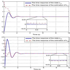
Simulation in Figures 1-2shows the system state variables and their estimations in presence of unknown time varying parameters Θ1(t) = Θ2(t) = 0.3t, and

simulation in Figures3-4shows that the system state variables and their estimations in presence of unknown time varying parameters Θ1(t) = Θ2(t) = 0.6t. The

estimation error between the states of the system (63 )-(68) and the states of the observer (69)-(74) converges to zero globally ultimately bounded. Therefore, zˆi=

col(ˆzi1,zˆi2)in (69)-(74) is an asymptotic estimation of

zi= col(zi1, zi2)in (63)-(68).

Remark 5. It should be noted that the states zˆi=

col(ˆzi1,zˆi2)in (69)-(74) give estimations of the variable

zi= col(zi1, zi2) in (63)-(68) for i= 1,2. From the

analysis in Sections II and III, it is straightforward to see thatxˆi = (TiTci)

−1_z_ˆ

i are estimations of the states

xi= [xi1 xi2]T of the system (52)-(55) whereTci and Tiare defined in(56)and(62)respectively fori= 1,2.

VI. Conclusion

An adaptive sliding mode observer for a class of nonlinear large scale interconnected systems with unknown TVPs has been proposed based on Lyapunov

c

(9)

Fig. 1. The time response of the 1st subsystem states and their estimates withΘ1(t) = Θ2(t) = 0.3t 0 2 4 6 8 10 −3 −2 −1 0 1 2 3 Time (s)

The time response of the state z21 The time response of the estimation of z21

0 2 4 6 8 10 −2 −1.5 −1 −0.5 0 0.5 1 1.5 2 2.5 Time (s)

Fig. 2. The time response of the 2nd subsystem states and their estimates withΘ1(t) = Θ2(t) = 0.3t

direct method. Although bounds on the unknown TVPs are not required, the rate of changes of these parameters are bounded. The technique that used in this paper is combined of sliding mode techniques and adaptive techniques to guarantee the ultimate boundedness of the estimation error of the designed observer. Simulation example has shown that the method is effective.

REFERENCES

1. Bakule L. “Decentralized control: An overview”. Annual Reviews in Control;32(1):87–98 (2008).

0 1 2 3 4 5 6 7 8 9 10 Time (s) -3 -2 -1 0 1 2 3

0 0.5 1 1.5 2 2.5 3 3.5 4 4.5 5 Time (s) -2 -1.5 -1 -0.5 0 0.5 1 1.5 2 2.5

Fig. 3. The time response of the 1st subsystem states and their estimates withΘ1(t) = Θ2(t) = 0.6t 0 0.5 1 1.5 2 2.5 3 3.5 4 4.5 5 Time (s) -3 -2 -1 0 1 2 3

0 0.5 1 1.5 2 2.5 3 3.5 4 4.5 5 Time (s) -2 -1 0 1 2 3 4 5

Fig. 4. The time response of the 2nd subsystem states and their estimates withΘ1(t_{) = Θ2}₍t_{) = 0}.₆t

2. Yan XG, Spurgeon SK, Edwards C. “Variable-Structure Control of Complex Systems: Analysis and Design”. Springer; (2017).

3. Mohamed M, Yan XG, Spurgeon SK, Jiang

B. “Robust sliding-mode observers for

large-scale systems with application to a multimachine

power system”. IET Control Theory &

Applications;11(8):1307–1315 (2016).

4. Liu WJ. “Decentralized Observer Design for a Class of Nonlinear Uncertain Large Scale Systems

with Lumped Perturbations”. Asian Journal of

Control;18(6):2037–2046 (2016).

c

(10)

9

5. Han W, Wang Z, Shen Y, Qi J. “L Observer

for Uncertain Linear Systems”. Asian Journal of Control. 2018;.

6. Wang YW, Zhang WA, Dong H, Zhu JW. Generalized Extended State Observer Based Control for Networked Interconnected Systems with Delays. Asian Journal of Control. 2018;.

7. Besanc¸on G. “Remarks on nonlinear adaptive

observer design”. Systems & Control

Let-ters;41(4):271–280 (2000).

8. Kreisselmeier G. “Adaptive observers with expo-nential rate of convergence”. IEEE Transactions on Automatic Control;22(1):2–8 (1977).

9. Cho YM, Rajamani R. “A systematic approach to adaptive observer synthesis for nonlinear

systems”. IEEE Transactions on Automatic

Control;42(4):534–537 (1997).

10. Marine R, Santosuosso GL, Tomei P. “Robust

adaptive observers for nonlinear systems with

bounded disturbances”. IEEE Transactions on

Automatic Control;46(6):967–972 (2001). 11. Liu Y. “Robust adaptive observer for nonlinear

systems with unmodeled dynamics”.

Automat-ica;45(8):1891–1895 (2009).

12. Yu L, Zheng G, Boutat D. “Adaptive observer for simultaneous state and parameter estimations for an output depending normal form”. Asian Journal of Control;19(1):356–361 (2017).

13. Bastin G, Gevers MR. “Stable adaptive observers

for nonlinear time-varying systems”. IEEE

Transactions on Automatic Control;33(7):650– 658 (1988).

14. Farza M, Bouraoui I, Menard T, Abdennour

RB, MSaad M. “Adaptive observers for a

class of uniformly observable systems with nonlinear parametrization and sampled outputs”. Automatica;50(11):2951–2960 (2014).

15. Kenn´e G, Ahmed-Ali T, Lamnabhi-Lagarrigue

F, Arzand´e A. “Nonlinear systems

time-varying parameter estimation: Application to

induction motors”. Electric Power Systems

Research;78(11):1881–1888 (2008).

16. Mohamed M, Yan X, Mao Z, Jiang B. “Adaptive Observer Design for a Class of Nonlinear Inter-connected Systems with Uncertain Time Vary-ing Parameters”;IFAC Papers Online;50(1):1421– 1426 (2017).

17. Edwards C, Yan XG, Spurgeon SK. “On

the solvability of the constrained Lyapunov

problem”. IEEE Transactions on Automatic

Control;52(10):1982–1987(2007).

18. Galimidi A, Barmish B. “The constrained

Lyapunov problem and its application to robust

output feedback stabilization”. IEEE Transactions on Automatic Control;31(5):410–419 (1986). 19. Deng F, Chen J, Chen C. “Adaptive unscented

Kalman filter for parameter and state estimation

of nonlinear high-speed objects”. Journal of

Systems Engineering and Electronics;24(4):655– 665 (2013).

20. Zhang Y, Zhang C, Zhang X.

“State-of-charge estimation of the lithium-ion battery system with time-varying parameter for hybrid

electric vehicles”. IET Control Theory &

Applications;8(3):160–167 (2013).

21. Edwards C, Spurgeon S. “Sliding mode control: theory and applications”. Crc Press(1998); 1998. 22. Utkin V, Guldner J, Shi J. “Sliding mode control

in electro-mechanical systems”. vol. 34. CRC

press; (2009).

23. Efimov D, Edwards C, Zolghadri A. “Enhance-ment of adaptive observer robustness applying

sliding mode techniques”. Automatica;72:53–56

(2016).

24. Yan XG, Edwards C. “Fault estimation for

single output nonlinear systems using an adaptive sliding mode estimator”. IET Control Theory & Applications;2(10):841–850 (2008).

25. Yan XG, Edwards C. “Adaptive

sliding-mode-observer-based fault reconstruction

for nonlinear systems with parametric

uncertainties”. IEEE Transactions on Industrial Electronics;55(11):4029–4036 (2008).

26. Lin S, Zhang W. “An adaptive sliding-mode

observer with a tangent function-based PLL structure for position sensorless PMSM drives”. International Journal of Electrical Power & Energy Systems;88:63–74 (2017).

27. Chen F, Zhang K, Jiang B, Wen C. “Adaptive Sliding Mode Observer-Based Robust Fault Reconstruction for a Helicopter With Actuator

Fault”. Asian Journal of Control;18(4):1558–

1565 (2016).

28. Laghrouche S, Liu J, Ahmed FS, Harmouche

M, Wack M. “Adaptive second-order sliding

mode observer-based fault reconstruction for PEM

fuel cell air-feed system”. IEEE Transactions

on Control Systems Technology;23(3):1098–1109 (2015).

29. Chen X, Park JH, Cao J, Qiu J. “Adaptive

synchronization of multiple uncertain coupled chaotic systems via sliding mode control”. Neurocomputing;273:9–21 (2018).

c

(11)

30. Yan XG, Edwards C. “Robust sliding mode observer-based actuator fault detection and isola-tion for a class of nonlinear systems”. Interna-tional Journal of Systems Science;39(4):349–359 (2008).

c