Forecasting in an extended chain-ladder-type model
1 Di KuangAon, 8 Devonshire Square, London EC2M 4PL, U.K. [email protected]
Bent Nielsen
Nuffield College, Oxford OX1 1NF, U.K. [email protected]
and Jens Perch Nielsen
Cass Business School, City University London, 106 Bunhill Row, London EC1Y 8TZ, U.K.
[email protected] 24 June 2010
Summary: Reserving in general insurance is often done using chain-ladder-type methods. We propose a method aimed at situations where there is a sudden change in the economic environment affecting the policies for all acci-dent years in the reserving triangle. It is shown that methods for forecasting non-stationary time series are helpful. We illustrate the method using data published in Barnett and Zehnwirth (2000). These data illustrate features we also found in data from the general insurer RSA during the recent credit crunch.
Keywords: Calendar effect, canonical parameter, extended chain-ladder, identification problem, forecasting.
1
Introduction
We consider chain-ladder-type models extended with a calendar effect used for reserving in general insurance as suggested by Zehnwirth (1994). The model describes the logarithm of claims in a log-additive form, involving three interlinked time scales for accident year, development year and calendar year. Due to the interlinkage of the three time scales the parameters of the model are not identified. A similar problem occurs in the age-period-cohort model used in demography, economics epidemiology and sociology. The identifica-tion problem has often been addressed by introducing somewhat arbitrary
restrictions on the parameters, which in turn can introduce some arbitrari-ness in the interpretation of estimators and in forecasts. Kuang, Nielsen and Nielsen (2008a,b) have proposed a canonical parametrisation that is uniquely identified and have shown how the arbitrariness in interpretations and fore-casts can be overcome. Given that analysis we are, in this paper, concerned with forecasting the calendar effect in a changing world such as in the cur-rent credit crunch. We therefore combine the canonical parametrisation with results from the literature on forecasting of non-stationary time series.
The log-normal version of chain-ladder, see Kremer (1982), Verrall (1994), immediately lends itself to the regression approach considered in this paper. The log-normal model deviates somewhat from the Poisson model that gives rise to the standard chain-ladder method, see Kuang, Nielsen and Nielsen (2009). While the standard chain-ladder is closely related to the log-normal approach of this paper, it does contain some additional challenges, see Bar-nett, Zehnwirth and Odell (2008). For clarity we therefore restrict ourself to the log-normal approach to chain-ladder-type models in this paper.
In a typical reserving setup, incremental claims data, Yij, are available
over a triangular index set I so the accident year, i, and the development year, j, satisfy 1 ≤ i, j ≤ k with i+j−1 ≤ k. The problem is to forecast the reserve over the lower triangle, where 1≤i, j ≤k so i+j −1> k. The extended chain-ladder-type model evolves around a parametrisation
µij =αi+βj +γi+j−1+δ, (1)
where αi is an accident year parameter, βj is a development year parameter,
γi+j−1 is a calendar year parameter, and δ gives the overall level. Thus, to
construct the forecasts it suffices to extrapolate the γ-parameters whereas estimates of the α, β and δ-parameters are readily available.
The standard chain-ladder-type model arises if the calendar parameters,
γ` can be set to zero in (1). This happens, for instance, if there is a constant
non-zero claims inflation, so γ` = c+d` for some constants c, d. In that
case it is possible to rewrite (1) as µij = ˘αi+ ˘βj + ˘δ, see §2, corresponding
to a standard chain-ladder-type model. Thus, the benefit of the extended model is the ability of incorporating a claims inflation which develops in a non-linear way.
The parametrisation (1) corresponds to the age-period-cohort parametri-sation. Important contributions in that direction have been made in demog-raphy and epidemiology by Berzuini and Clayton (1994), Carstensen (2007),
Clayton and Schifflers (1987), Keiding (1990), in economics by Deaton and Paxson (1994) and in sociology by Yang, Fu and Land (2004). We use the parametrisation described by Kuang, Nielsen and Nielsen (2008a,b), which can be applied in all these situations, in combination with the techniques for forecasting non-stationary time series discussed by Clements and Hendry (1999), see also Hendry and Nielsen (2007, §21) for a more introductory reference.
Clements and Hendry (1999) consider the problem of forecasting when there are structural changes out of sample. That is the situation where a model describes the data in sample, but fails to capture important features of data out of sample. This could for instance arise because of changes in legislation, in the business setup, or in the economic environment. The data will typically not be informative about such changes, but the actuary may have additional information that is external to the data. Clements and Hendry (1999) discuss various forecast methods that work well in presence of structural changes out of sample. If structural changes are expected it is typically better to forecast growth rates or accelerations rather than levels. This comes at a modest cost when there are no structural changes, but with potentially large gains when changes occur. The investigator can often choose between these methods using patterns of the most recent observations along with substantive information which is external to data.
We propose to construct the reserve forecasts through a two-step estima-tion procedure. In a first step the parameters of the model are estimated using linear regression. In a second step the actuary looks at the estimated calendar parameters in conjunction with information external to the data. The point explored by Kuang, Nielsen and Nielsen (2008a,b) is that the cal-endar parameters are only determined up to an arbitrary linear trend. Thus, when transferring the findings of Clements and Hendry (1999) we will focus on features over and above linear trends. Thus, the level approach corre-sponds to extrapolating the linear trend, more or less as in the standard chain-ladder. The growth approach and, in particular, the acceleration ap-proach will be beneficial when the calendar parameter develops differently from a linear trend. These forecast methods may give different forecast sce-narios. Based on the actuary’s analysis it is often possible to give more weight to some scenarios than to other scenarios.
Using a simulation study we show how these findings from time series analysis carry over to the reserving problem. When applying our forecast-ing technique on real data, we see that when the calendar parameters are
behaving in a relatively stable way while the growth rate and acceleration approaches predicts slightly worse than the level approach. However, when the time series is really challenging with a rapid change over a short period of time, then only a growth rate approach or an acceleration approach perform well when forecasting. We suggest to compute all approaches and choose between them using acturial judgement. Our approach is based on micro data from insurance. For a macro analyses of the impact of changes in loss ratios see Barth and Eckles (2009).
An important point of the analysis is that the data will not contain in-formation about the forecast period so acturial judgement will have to be based on external information. The actuary may have various types of in-formation at hand. For instance, in the recent credit crunch the crisis could affect different business lines differently and the crisis could hit some geo-graphical areas before other areas. This type of information play into the different forecast scenarios offered with the presented method and give the actuary a way of working quantitatively with external information. Indeed, our methods were used in this way by the global general insurer RSA in the recent credit crunch. For an analyses of the credit crunch crises in a wider insurance related context, see Harrington (2009).
The paper is organised so that the method is introduced in§2, by first de-scribing the data and the extended chain-ladder-type model, then discussing the identification problem and the time series forecast methods. The prob-lem of forecasting under structural change is analysed in a toy model in §3, analysed through simulation in §4, and illustrated with reserving data from general insurance in §5. §6 concludes.
2
The forecast method
We start by describing the data and the extended chain-ladder-type model. The chain-ladder-type models have an inherent identification problem. For the estimation and the forecast analysis it is useful to review the recent results of Kuang, Nielsen and Nielsen (2008a,b) concerning the identification and forecast of parameters in the presence of this identification problem.
2.1
The data
In this study we are concerned with a standard reserving problem. An in-troduction to the reserving problem is found in England and Verrall (2000) and we assume that aggregated data is available and that these aggregates are lognormally distributed. Frequencies or zero claims do not enter our aggregated analysis, see also Boucher, Denuit and Guillen (2009). Thus, in-cremental data for the severity or the number of claims,Yij are available over
a triangular index set I so the accident year, i, and the development year, j, satisfy 1≤i, j ≤k with i+j−1≤k.
In the empirical illustration a reserving triangle of dimensionk = 11 from Barnett & Zehnwirth (2000, Table 3.5) is used.
2.2
The statistical model
When constructing a statistical model we first of all assume that the variables
Yij are independent as they represent incremental claims data. We assume
Yij has a log normal distribution. Thus, logYij is normally distributed with
log density logf(yij) = − 1 2log(2πσ 2)− 1 2σ2(yij −µij) 2,
where µij was defined in (1) and σ2 is the variance parameter. The reduced
model where the calendar year effect, γi+j−1, is absent corresponds to the
chain-ladder-type model discussed by for instance Kremer (1982) and Verrall (1991, 1994).
2.3
Identification
The parametrisation (1) has a well-documented identification problem in that arbitrary constants and an arbitrary linear trend can be added to the elements of the (3k+ 1)-dimensional parameter
θ = (α1, . . . , αk, β1, . . . , βk, γ1, . . . , γk, δ)0 (2)
without changing µij. As described by Carstensen (2007) the parameter µij
is invariant to the group of transformations
g : αi βj γi+j−1 δ 7→ αi+a+ (i−1)d βj +b+ (j −1)d γi+j−1+c−(i+j −2)d δ−a−b−c , (3)
for arbitrary constants a, b, c and d, that is µ(θ) = µ{g(θ)}. Since µ is in-variant to the transformation of g it would be natural to look for a function of θ that is invariant to g and which captures the variation of µover the pa-rameter space. Cox & Hinkley (1974, §5.3) give an overview of the invariance terminology. Kuang, Nielsen and Nielsen (2008a) propose such a function.
The proposal is a canonical parameter ξ of dimension (3k−3). The
motivations for the parametrisation stems from writing
µij = µ11+ (i−1)(µ21−µ11) + (j−1)(µ12−µ11) + i X t=3 t X s=3 ∆2αs+ j X t=3 t X s=3 ∆2βs+ i+jX−1 t=3 t X s=3 ∆2γs (4)
for all i, j ∈I, where ∆αi =αi−αi−1 and ∆2αi = ∆αi−∆αi−1, so i X t=3 t X s=3 ∆2αs= i X s=3 (i−s+ 1)∆2αs. (5)
The candidate canonical parameter is therefore
ξ= (µ11, µ21, µ12,∆2αi,∆2βj,∆2γ` for 3≤i, j, ` ≤k)0 ∈R3k−3. (6)
The interpretation derives from (4) so thatµ11determines the level,µ12−µ11
and µ12−µ11 determines linear effects such as a constant claims inflation,
while the double differenced parameters determines the non-linear effects. The parameterξ is a function of θ as defined in (2) and it is invariant to
g soξ(θ) = ξ{g(θ)}as desired. Kuang, Nielsen and Nielsen (2008a, Theorem 1) show that the canonical parameter gives a unique parameterization of µ, so that for ξ† 6=  then µ(ξ†) 6= µ(). In other words, the canonical parameter ξ is a maximal invariant ofθ under the transformationsg.
Parametersαi,βj,γi+j−1 andδcan be constructed from (3), (4) to satisfy
arbitrary identification schemes. For instance, the frequently used identifica-tion scheme α†1 =β1† =γ1† =γ2† = 0 can be imposed by letting
α†i = i X t=3 t X s=3 ∆2α s+ (i−1)(µ21−µ11), βi† = j X t=3 t X s=3 ∆2βs+ (j−1)(µ12−µ11), γ†i = i+jX−1 t=3 t X s=3 ∆2γ s, δ† =µ11.
Another frequently used identification scheme is Pki=1ᆆi = Pkj=1βj†† =
Pk
s=1γs†† =䆆 = 0, which is imposed by (ᆆi , βj††, γs††, 䆆) = g(α†i, βj†, γs†, δ†),
where (a, b, c, d) is chosen as the unique solution of the linear system
k 0 0 Pki=1(i−1) 0 k 0 Pki=1(i−1) 0 0 k Pki=1(i−1) 0 0 1 −1 a b c d + Pk i=1α † i Pk j=1β † j Pk s=1γs† δ† = 0.
Working with any such arbitrary identification may have bearing on inter-pretation and on forecasts.
2.4
Estimation
The log normal chain-ladder model is a linear regression model. To exploit this feature in the estimation stack the data logYij as a vector of dimension
k(k+ 1)/2. The design matrix, X, is of dimension {k(k+ 1)/2} ×(3k−3) and can be defined from the equations (4), (5). The row of X corresponding to observation i, j has the form
Xij ={1, i−1, j−1, h(i,3), . . . , h(i, k), h(j,3), . . . , h(j, k),
h(i+j−1,3), . . . , h(i+j −1, k)}, (7) whereh(i, s) = max(i−s+ 1,0). The parameters of the model are estimated by least squares regression of log(Yij) on the design Xij.
The regression approach has various well-known properties. In the con-text of the log-normal model it delivers maximum likelihood estimators which are unbiased estimators for the parameters of interest. In other words the expectation of the logged data, ElogYij, is estimated without bias. This
translates into unbiased estimators for the median of the original data Yij.
Due to the Jensen inequality, the estimator for the expectation of the original data, EYij, will, however, be biased.
2.5
Forecast methods
Kuang, Nielsen and Nielsen (2008b) characterise forecasts of µij that are
invariant to arbitrary identifications of the parameters αi, βj, γi+j−1 and δ.
trend inγi+j−1 the forecastsγek+h of γk+h need to have a particular structure:
it should be a sum of two components, of which the first exactly extrapolates the arbitrary linear trend and the second is invariant to the linear trend. We will consider three such forecasts.
The forecasts methods originate from the forecasting techniques for non-stationary time series discussed by Clements and Hendry (1999, §5). There are time series that are easier to predict than others. When the time series is well behaved around the arbitrary linear trend many types of forecast models will do well. However, when the time series appears to have structural shifts or where structural shifts may occur out of sample then forecasting is more difficult. The forecaster can then choose between two main strategies: either to do extremely well when structural shifts are modest, which is perhaps the most typical outcome, but perform very poorly when structural shifts occur or to choose a strategy that performs slightly worse when nothing happens but a lot a better when structural shifts occur.
It is important to be aware that in our case we do not observe the time series directly, as the time series analysed is extracted as parameter estimates from a statistical model. Thus, our method is a two step approach, first a model is fitted and the calendar effect is extracted, then this estimated cal-endar effect is analysed as a time series and extrapolated. The parameter µij
is then forecasted by combining the estimates for accident year, development year and level with the forecast of the calendar effect.
In the following we focus on the forecasting in the second step and discuss three different methods. For convenience let xt, t = 1, . . . , k denote the
extracted time series. Due to the identification problem the time series will evolve around an arbitrary linear trend.
The first forecast model is suited for the situation where the time series evolves in a stable way both in-sample and out-of-sample. The idea is then to extrapolate the linear trend in the data using the forecast model xt =
µ+νt+εt. Here,εtrepresents a sequence of independent, normally,N(0, ω2
)-distributed innovations. In situations with many observations this could be augmented with a autoregressive structure. The h-step-ahead point forecast is then e xk+h =ϕb+ (k+h)bν, where bν={Pkt=1xt(t−t)}/{ Pk t=1(t−t)2}and ϕb=k−1 Pk t=1(xt−bνt), with t =k−1Pk
t=1t. Density forecasts can be constructed by adding a normal,
N(0,ωb2)-distributed variable e²
t+h, whereωb2 =k−1
Pk
The second forecast model is suited for the situation where there is a level shift in the forecast period. In that situation the growth rates or differences of the time series can be forecasted using a random walk model of the type ∆xt=η+εt and gives a h-step-ahead point forecast of
e
xk+h =xk+hbη,
where bη= (k−1)−1Pk
t=2∆xt. Again, density forecasts can be constructed
by adding a normal, N(0, hωb2)-distributed variable e²
t+h, with variance
esti-mator ωb2 = (k−1)−1Pk
t=2(∆xt−bη)2.
The third situation we study is where there is a slope shift of the linear trend in the forecast period. In that case, we could apply the forecast model ∆2x
t=εtfor the accelerations or double differences. Theh-step-ahead point
forecast is then
e
xk+h =xk+h∆xk.
Density forecasts can be constructed by adding aN(0,ωb2Ph
i=1i2)-distributed
variable e²t+h, whereωb2 = (k−2)−1
Pk
t=3(∆2xt)2.
It is convenient to refer to these time series models by their order of integration. This terminology is used in the econometric analysis of linear time series to classify non-stationary time series that become stationary by differencing d times. Thus, the three forecast models are I(0), I(1) and I(2)-models.
3
A toy model for structural changes in the
forecasts period
We will now look at the performance of the forecast methods towards struc-tural changes in the calendar effect during the forecast period. As we would like to cover a variety of different types of structural changes a formal analysis would be rather involving. Instead we follow the approach of Clements and Hendry (1999) and work through examples. These example are chosen in a rather simple fashion and yet, these are informative about the issues faced in applied work. Due to the invariance features of the problem the scenario of a constantly sloping linear trend can be captured by choosing γ` = 0. The
stylised version of structural change is when the calendar effect is zero for a while and then changes. If the findings of Clements and Hendry (1999) carry over this is precisely a situation where forecast failures can be severe. They
1 k−1 k k+1 0 z 2z (a) Scenario 0 1 k−1 k k+1 0 z 2z (b) Scenario 1 1 k−1 k k+1 0 z 2z (c) Scenario 2
Figure 1: Forecast scenarios. Panels show γ` as function of`. The in-sample
period is 1≤` ≤k.
analysed the sources of possible forecast failure in non-stationary time series and found the most important sources to be structural changes in the level or slope of a time series rather than changes in the dynamic parameters.
The situation where the process has a constant level in sample and jumps out of sample is most difficult to address as the investigator finds no warning from the data. We therefore turn to the more manageable situation in which the level jumps in the last in-sample period. While the sample does not give any information about the out-of-sample period, the actuary is prompted to look for external information that will help in deciding on the preferable method required for the forecast.
In the remainder of the paper we focus on one-step ahead forecasts of the calendar effect rather than forecasts of the full lower triangle. This is in part to be able to investigate the performance of the method on real data and in part because multi-step forecasting involves additional issues as documented by Clements and Hendry (1999).
The situation we have in mind is when the estimated γ-series has an
outlier in the last in-sample period. For simplicity let the calendar parameter be zero for all but the last in-sample calendar year,γ` = 0 for` = 1, . . . , k−1,
but take a non-zero value in the last in-sample period, γk = z. Since γ1 =
γ2 = 0 the γ-series is identified so γ` =
P`
t=3
Pt
s=3∆2γs. We will study the
performance of the three forecast models under three different out-of-sample scenarios, illustrated in Figure 1, in which the first out-of-sample value is
γk+1 =zdin scenariodford= 0,1,2. Thus, in scenario 0, thenγ drops back
to zero,γk+1 = 0, in scenario 1 it stays at the new level,γk+1 =z, in scenario
Scenario 0 1 2 I(0)-forecast 4/k 4/k−1 4/k−2 I(1)-forecast 1/(k−1) + 1 1/(k−1) 1/(k−1)−1
I(2)-forecast 2 1 0
Table 1: Forecast errors for different experiment. Proportionality factors are reported, which should be multiplied by z to get total effect.
I(d)-forecast model will fare best in scenario d.
When z = 0 the forecasts of the three forecast models, xeI(0)k+1, xeI(1)k+1, and
e
xI(2)k+1, are all zero. When z 6= 0 these forecasts changes. For instance, the I(2)-forecast is eγk+1I(2) =γk+ ∆γk=z+ (z−0) = z2. Overall we have
e
γk+1I(0) 7→z4/k, eγk+1I(1) 7→z{1/(k−1) + 1}, eγk+1I(2) 7→z2.
It is then straight forward to calculate the forecast error for scenariodwhere the actual outcome is zd. These errors are reported in Table 1. Table 1 shows that for scenario d forecast method d is preferable, as long as k ≥6.
At first the above analysis may seem overly simplistic. However, through a simulation study and through an empirical example the analysis turns out to be informative about practical issues faced by actuaries.
4
Simulation of structural change in the
fore-cast period
We now turn to a simulation study to further illustrate the effects of struc-tural changes on forecasts. In the simulation design the accident and de-velopment parameters are chosen to match the empirical illustration in §5, while the calendar parameters will change according to the scenarios set up in §3. The finding that an I(d)-forecast is preferable in scenario d will be seen to carry over.
The simulation model is constructed as follows. The data areYij wherei, j
vary in the triangular index setI so 1 ≤i, j ≤k soi+j−1≤k withk = 11, whereas the out-of-sample data is the first diagonal of the lower triangle
for calendar year k + 1 corresponding to index set J where 2 ≤ i, j ≤ k
so i+j −1 = k + 1. It is assumed that logYij is N(µij, σ2)-distributed.
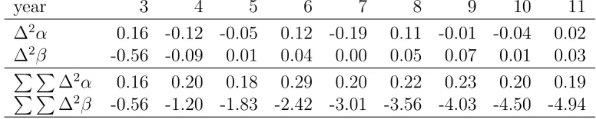
year 3 4 5 6 7 8 9 10 11 ∆2α 0.16 -0.12 -0.05 0.12 -0.19 0.11 -0.01 -0.04 0.02 ∆2β -0.56 -0.09 0.01 0.04 0.00 0.05 0.07 0.01 0.03 P P ∆2α 0.16 0.20 0.18 0.29 0.20 0.22 0.23 0.20 0.19 P P ∆2β -0.56 -1.20 -1.83 -2.42 -3.01 -3.56 -4.03 -4.50 -4.94
Table 2: Values of the canonical parameter for the first experiment. All calendar parameters are zero, ∆2γ
j = 0, for j = 3, . . . , k+ 1. The level and
growth rates are determined byµ11= 11.05,µ21−µ11= 0.09,µ12−µ11= 0.25.
The variance is σ2 = 0.0047.
i +j −1 = k + 1. Three experimental designs are made. Recalling the
canonical parametrisation in (6) these designs are constructed as follows. The parameters αi, βj, µ11, µ12, µ21, σ2 takes the values reported in Table 2
and are actually estimates from the empirical illustration in §5, while γ`
is chosen as described in §3. In each of 104 repetitions independent log
normally distributed variablesYij are generated over the index setsI and J.
An estimate for the canonical parameter ξ is then found by applying least squares regression to the logarithm of the observations, log(Yij), on the design
matrix defined in (7). The calendar parameter, γ`, is then extrapolated using
one of the three forecast methods outlined in §2. This, in turn, results in forecastsµeij over the index setJ, and median-unbiased forecasts exp(µeij) for
Yij follow. Since σ2 is so small in this setup forecasts of the expectation
exp(µeij+σ2/2) would be nearly identical. For each element inJ the squared
forecast error is computed and the square roots of the averages of these are reported. Similarly, the average of the absolute errors in forecasting the sum of the elements in J is computed.
Table 3 shows results from the benchmark case, where z = 0 so there
are no structural change neither in-sample nor out-of-sample. All forecast methods fare quite well, although there is some cost when moving from an I(0)-forecast model to an I(1) or an I(2)-forecast model. The experimental design has increasingly negative age-parameter, βj, see Table 2, and thus
exp(βj) is strongly declining. The largest observations and hence the largest
forecast errors then appear for small age values. TheI(0)-forecast model has, uniformly accross j, the smallest forecast error.
For comparison Table 3 also shows the outcomes from forecasting using a model with a two-dimensional parametrisation where the calendar
parame-age, j 2 3 4 5 6 7 8 9 10 11 all
I(0)-forecast 26 15 9 5 3 2 2 1 1 1 33
I(1)-forecast 25 15 9 5 4 2 2 1 1 1 33
I(2)-forecast 27 17 10 6 4 3 2 1 1 1 43
2-dimensional model 25 15 9 5 3 2 1 1 1 1 32
Table 3: Simulated forecast errors in the benchmark case where z = 0.
For 2 ≤ j ≤ 11 the root of mean of squared errors in forecasting Y13−j,j is
reported. Last column shows mean absolute error in forecastingP12j=2Y13−j,j.
First panel shows forecasts fromI(d)-forecast models. For comparison, second panel shows forecasts from the 2-dimensional model with restriction γ` = 0
imposed. A scale of 103 is omitted. Based on 104 repetitions.
tersγ`are restricted to be zero. As above the model is estimated by regression
over the index setI, giving the chain-ladder-type estimates of Kremer (1982). When forecasting over J estimates are available for all parameters and there is no need for any extrapolation. It is seen that when the calendar parameter is zero the forecasts are a slightly improved version of the I(0)-forecasts.
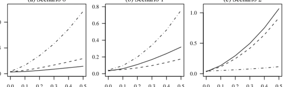
Figure 2 shows outcomes for the three different scenarios. Only the av-erage forecast errors for the sum of elements in J is shown; the results are nearly identical for individual elements. For each scenario the average fore-cast error is shown as a function of the size of structural break, z. To get an idea of the units of z, note that the standard error of the simulated normal distributions are σ = 0.00471/2 = 0.07. The graphs confirm the finding from
§3 that the I(d)-forecast method is preferable in scenariod.
If the two-dimensional model had been used in this situation the outcome would have been similar to those of the I(1)-forecast. The result is, however, more subtle than that. The nature of the forecast-failure is quite different. Whereas the three-dimensional model is well-specified in the forecast period, but with a structural break in the mean, the two-dimensional model is actu-ally mis-specified. Thus, the forecast failure for the two-dimensional model is of different character for different elements in the setJ. Plots like those in Figure 2 for individual elements in J would be similar for the I(d)-forecasts. The two-dimensional forecast, however, would be similar to I(1)-forecasts for extreme elements of J with a low or a high age index, whereas it would be similar to I(0)-forecasts for a medium value of the age index. As the values for low age indices dominate in this example theI(1)-like forecasts dominate the aggregated result.
0.0 0.1 0.2 0.3 0.4 0.5 0.0 0.5 1.0 (a) Scenario 0 0.0 0.1 0.2 0.3 0.4 0.5 0.0 0.2 0.4 0.6 0.8 (b) Scenario 1 0.0 0.1 0.2 0.3 0.4 0.5 0.0 0.5 1.0 (c) Scenario 2
Figure 2: Simulated forecast errors for the three scenarios. The mean ab-solute error in forecasting P12j=2Y13−j,j is shown as a function of the size of
the structural break, z. The I(0)-forecast is shown with solid line. The I(1)-forecast is shown with dashes. The I(2)-forecast is shown with dash/dots. The forecast errors should be scaled by 106.
5
Empirical illustration of structural change
in the forecast period
The lessons from above are now applied to thek = 11 dimensional reserving data of Barnett & Zehnwirth (2000, Table 3.5) as suggested in §2. The lessons are particular helpful if the actuary can identify whether one of the scenarios d apply. Indeed if scenario d applies forecast errors are reduced by choosing the I(d)-forecast.
We can ignore the so-called exposure factor due to an invariance prop-erties of the log normal model. The reason is that the log-normal model is estimated by least squares regression of the logged observations on a design matrix defined from (4). An exposure factor is multiplicative on the original scale and additive on the logged scale. The linearity of the least squares estimator then implies an invariance to the exposure factor. This argument applies not only to exposure factors on the accident year scale, but also to known inflation factors on the calendar scale as well as to known factors on the development scale. To be precise, suppose a datasetYij overI has
maxi-mum likelihood estimator ˆξ for the canonical parameter (6). Let ξ† ∈R3k−3
and construct µ†ij using (4). Then the data Yij† =Yijexp(µ†ij) has maximum
likelihood estimator ˆξ+ξ†. The same argument would apply ifξ†were defined for instance from the exposure factor.
1 3 5 7 9 11 0.0 0.1 0.2 0.3 0.4
Figure 3: Estimated calendar parameters, γ`, based on data from Barnett &
Zehnwirth (2000, Table 3.5). The γ-series is identified soγ1 =γ2 = 0.
forecasts. The idea is to consider a subset of the data consisting of the m
first calendar years, which gives an m-dimensional triangle, Im. The model
is estimated on the triangle Im and used to forecast the entries Jm+1 for
calendar year m+ 1, where 2 ≤i≤m and j =m−i+ 2. This will be done for m= 5, . . . ,10.
Fitting a log normal model without calendar effect, γ` = 0 for all `, by
least squares regression results in the estimates reported in Table 2. Fitting a log normal model with calendar effect gives slightly different estimates for the
α- and theβ-series, as well as the γ-series reported in Figure 3. Looking at Figure 3 until year 7 indicates a more or less linear development. Year 8 is a bit out, but then at year 9 it is back at the same linear trend line. It appears that the linear trend line is broken with a new slope in years 10 and 11. In terms of the analysis of §3 one step forecasts at m = 5,6,7,8 appear to be of scenario 0, but with some noise for m= 8 and perhaps also m= 7. Then the trend line changes and forecasts at m = 9,10 appear to be of scenario 2. There is a nearly straight line through the points at m= 9,10,11 indicating that an I(2) will work particularly well when forecasting from m = 10.
Table 4 shows the actual one-step-ahead point forecasts produced by the two-step approach outlined above. It is seen that the predictions of §3 are
matched exactly. For m = 9 and m = 10, which are like scenario 2, the
I(2)-forecast gives dramatic gains relative to the other methods.
For comparison Table 4 also show results for 2-dimensional model, where the calendar parameters,γ`, are restricted to be zero. This corresponds to the
forecast origin, m 5 6 7 8 9 10 actual outturn at m+ 1 644.2 709.8 723.7 864.5 1140.4 1478.6 I(0)-forecast -3.0 11.1 -4.8 57.2 163.2 264.2 I(1)-forecast -3.1 11.9 -11.0 72.4 138.0 139.7 I(2)-forecast -4.5 12.6 -18.0 93.5 88.5 -7.0 2-dimensional model -3.9 10.8 -8.1 63.3 152.1 195.7
Table 4: Forecast errors for reserving data. All figures should be scaled by
103. First panel shows actual outcomes. Second panel shows the actual
1-step-ahead forecast errors for Pmj=1−1(Yem−j,j+1 −Ym−j,j+1) using three
dif-ferent forecast methods for extrapolating γ` in order to get median unbiased
forecasts. For each m the smallest forecast error is indicated by bold face. Third panel shows the result of forecasts from a 2-dimensional model with restriction γ` = 0 imposed.
chain-ladder type model of Kremer (1982). The likelihood ratio test statistic is 120.5 for this restriction of 9 degrees of freedom. While this indicates that the restricted model is mis-specified, parsimoneous models are often found to perform well in forecasting. The forecast results are in the same range as the I(0)-forecasts for all forecast origins, matching the discussion in §4.
In practice, the insurance company would be interested in forecasting the entire lower triangle J. Typically the largest entries of J would be in the first out-of-sample calendar year, so the one-step-ahead forecast would be very important to get right. As multi-step forecasting throw up some additional issues this is left for future work. In many situations the entries for small j would dominate as seen in Table 3, so the actuary can possibly even focus on forecasting a few cells.
6
Discussion
The main conclusion is that in a benign world with nearly constantly slop-ing calendar effects most forecasts methods do well with a two-dimensional method ignoring calendar effects or a three-dimensional method extrapolat-ing the calendar effect by an I(0) method comes out slightly better than other methods. Once the calendar effects has structural changes in the fore-cast period as could be experienced in the current credit crunch the growth rates forecasts and accelerations forecasts tend to give better forecasts than
level forecasts. In particular the I(2) can be a vast improvement over other methods. In practice the actuary is probably best off producing both I(0) and I(2) forecasts. In cases of major differences in the forecasts the actuary may apply judgement based on information external to the data.
The techniques studied here have scope for further work on various gen-eralisations. Multi-step forecasting is needed to forecast the full lower tri-angle. Likewise density forecasts would be of interest as opposed to the point forecasts considered here. The methods could be carried over to age-period-cohort-type data from other disciplines than general insurance. Such studies would typically have slightly different structures, which would have to be analysed on an individual basis. In some situations forecasts involving extrapolation of all of the accident, development and calendar-parameters would be of relevance.
The methods of this paper have been implemented during the summer of 2009 on a number of confidential reserving data sets from the major global insurer RSA. The methods work along the lines illustrated in this paper. However, the impact of the credit crunch varies a lot depending on the con-sidered business line as the credit crunch may have different implications depending on the business line. The effects of the current credit crunch is visible in the most recent calendar periods. Depending on whether these structural changes are judged to be permanent or transitory in the forecasts period the acceleration or the level approach would be appropriate to use. Overall, it appears that the suggested methods can address the major struc-tural changes non-life insurance companies are faced with right now.
References
Barnett, G., and B. Zehnwirth, 2000, Best estimates for reserves, Proceed-ings of the Casualty Actuarial Society, 87: 245–321.
Barnett, G., D. Odell, and B. Zehnwirth, 2008, Meaningful intervals, Casu-alty Actuarial Society Forum, Fall 2008: 16–52.
Barth, M.M., and D.L. Eckles, 2009, An empirical investigation of the effect of growth on short-term changes in loss ratios, Journal of Risk and Insurance, 76: 867–885.
Berzuini, C., and D. Clayton, 1994, Bayesian analysis of survival on multiple time scales, Statistics in Medicine, 13: 823–838.
Boucher, J.-P., M. Denuit, and M. Guillen, 2009, Number of accidents or number of claims? An approach with zero-inflated Poisson models for panel data, Journal of Risk and Insurance, 76: 821–846.
Carstensen, B., 2007, Age-period-cohort models for the Lexis diagram, Statistics in Medicine, 26: 3018–45.
Clayton, D., and E. Schifflers, 1987, Models for temporal variation in cancer rates. II: Age-period-cohort models, Statistics in Medicine, 6: 469–81.
Clements, M.P., and D.F. Hendry, 1999, Forecasting non-stationary time
series (Cambridge, MA: MIT Press).
Cox, D.R., and D.V. Hinkley, 1974, Theoretical Statistics (London: Chap-man and Hall).
Deaton, A.S., and C.H. Paxson, 1994, Saving, growth and aging in Taiwan, in D.A. Wise, ed.,Studies in the economics of aging(Chicago: Chicago University Press), pp. 331–357.
England, P.D., and R.J. Verrall, 2002, Stochastic claims reserving in general insurance, British Actuarial Journal, 8: 519–44.
Harrington, S.E., 2009, The financial crisis, systemic risk, and the future of insurance regulation, Journal of Risk and Insurance, 76: 785–819.
Hendry, D.F., and B. Nielsen, 2007, Econometric Modeling: A likelihood
approach (Princeton NJ: Princeton University Press).
Keiding, N., 1990, Statistical inference in the Lexis diagram, Philosophical Transactions: Physical Sciences and Engineering, 332: 487–509.
Kremer, E., 1982, IBNR-claims and the two-way model of ANOVA,
Scan-dinavian Actuarial Journal, 47–55.
Kuang, D., B. Nielsen, and J.P. Nielsen, 2008a, Identification of the age-period-cohort model and the extended chain-ladder model,Biometrika, 95: 979–986.
Kuang, D., B. Nielsen, and J.P. Nielsen, 2008b, Forecasting with the age-period-cohort model and the extended chain-ladder model,Biometrika, 95: 987–991.
Kuang, D., B. Nielsen, and J.P. Nielsen, 2009, Chain-ladder as maximum likelihood revisited, Annals of Actuarial Science, 4: 105–121.
R Development Core Team, 2006,R: A Language and Environment for
Sta-tistical Computing (Vienna: R Foundation for Statistical Computing).
Verrall, R., 1991, Chain-ladder and maximum likelihood, Journal of the
Institute of Actuaries, 118: 489–499.
Verrall, R., 1994, Statistical methods for the chain-ladder technique, Casu-alty Actuarial Society Forum, Spring 1994: 393–446.
Yang, Y., W.J. Fu, and K.C. Land, 2004, A methodological comparison of age-period-cohort models: The intrinsic estimator and conventional generalized linear models, Sociological Methodology, 34: 75–110. Zehnwirth, B., 1994, Probabilistic development factor models with
appli-cations to loss reserve variability, prediction intervals, and risk based capital, Casualty Actuarial Society Forum, Spring 1994: 447–605.