Modeling psychophysical data at the population-level:
The generalized linear mixed model
Alessandro Moscatelli
#
$
Center of Space BioMedicine, University of Rome‘‘Tor Vergata,’’ Rome, Italy Laboratory of Neuromotor Physiology, Santa Lucia Foundation, Rome, Italy Department of Cognitive Neuroscience, University of Bielefeld, Bielefeld, Germany
Maura Mezzetti
University of RomeDepartment of Economics and Finance,‘‘Tor Vergata,’’ Rome, Italy$
Francesco Lacquaniti
$
Center of Space BioMedicine, University of Rome‘‘Tor Vergata,’’ Rome, Italy Department of Systems Medicine, Neuroscience Section, University of Rome‘‘Tor Vergata,’’ Rome, Italy Laboratory of Neuromotor Physiology, Santa Lucia Foundation, Rome, Italy
In psychophysics, researchers usually apply a two-level model for the analysis of the behavior of the single subject and the population. This classical model has two main disadvantages. First, the second level of the analysis discards information on trial repetitions and subject-specific variability. Second, the model does not easily allow assessing the goodness of fit. As an alternative to this classical approach, here we propose the Generalized Linear Mixed Model (GLMM). The GLMM separately estimates the variability of fixed and random effects, it has a higher statistical power, and it allows an easier assessment of the goodness of fit compared with the classical two-level model. GLMMs have been frequently used in many disciplines since the 1990s; however, they have been rarely applied in psychophysics. Furthermore, to our knowledge, the issue of estimating the point-of-subjective-equivalence (PSE) within the GLMM framework has never been addressed. Therefore the article has two purposes: It provides a brief introduction to the usage of the GLMM in psychophysics, and it evaluates two different methods to estimate the PSE and its variability within the GLMM framework. We compare the performance of the GLMM and the classical two-level model on published experimental data and simulated data. We report that the estimated values of the parameters were similar between the two models and Type I errors were below the confidence level in both models. However, the GLMM has a higher statistical power than the two-level model. Moreover, one can easily compare the fit of different GLMMs according to different criteria. In conclusion, we argue that the GLMM can be a useful method in psychophysics.
Keywords: Generalized Linear Mixed Model, two-level analysis, psychophysics, statistical power
Citation: Moscatelli, A., Mezzetti, M., & Lacquaniti, F. (2012). Modeling psychophysical data at the population-level: The generalized linear mixed model.Journal of Vision, 12(11):26, 1–17, http://www.journalofvision.org/content/12/11/26, doi:10. 1167/12.11.26.
Introduction
The psychometric function relates the response of a subject to the magnitude of a physical stimulus. A
Generalized Linear Model (GLM; Agresti, 2002) is
usually applied to these data sets; in its simple form the model has two parameters, typically the intercept and the slope of the linear predictor. More sophis-ticated models have been proposed to take into
account lapses and guesses by the participant
(Wichmann & Hill, 2001a; Yssaad-Fesselier &
Knoblauch, 2006), and a priori hypotheses of the
experimenter (Kuss, J ¨akel, & Wichmann, 2005).
Ordinary GLMs, as well as other models of the kind mentioned above, assume that the responses are independent and conditionally identically distributed. While the responses of a single subject may approximately satisfy these assumptions, the repeated
responses collected from more than one subject generally do not. Actually, nonstationarities due to learning or fatigue, for example, may result in violations of these assumptions even in the case of a single subject: In this context, notice that a beta-binomial model has been proposed to deal with nonstationary responses (Fr ¨und, Haenel, &
Wich-mann, 2011). In the case of repeated responses from
more than one subject, ordinary GLMs treat the errors within subject in the same manner as the errors between subjects, and tend to produce invalid standard errors of the estimated parameters. A typical approach to overcome this problem consists in applying a two-level analysis (e.g., Morrone, Ross,
& Burr, 2005; Pariyadath & Eagleman, 2007;
Johnston et al., 2008). First, the parameters of the
psychometric function are estimated for each subject. Next, the individual estimates are pooled to perform the second-level analysis, and inference is carried out,
for example, by means oft test or ANOVA statistics.
As an alternative to this two-level approach, here we
propose the application of Generalized Linear Mixed
Models (GLMM; Cox, 1958; Rasch, 1961; Breslow &
Clayton, 1993; Agresti, 2002; Bolker et al., 2009;
Knoblauch & Maloney, 2012). The GLMM is an
extension of the GLM that allows the analysis of clustered categorical data, as in the case of repeated responses from different subjects. In the GLMM, the first and second levels of the analysis are implemented simultaneously. Some of the advantages of the GLMM with respect to the two-level analysis are: (a) the GLMM takes the whole ensemble of the responses as input data, (b) it separately estimates the variability of fixed and random effects, and (c) it allows an easier assessment of the goodness of fit.
GLMMs and related models have been frequently used in many disciplines since the 1990s, but they have been rarely used in psychophysics. The pertinent literature on related topics includes the following
references. Baayen, Davidson, and Bates (2008) and
Quene´ & van den Bergh (2008) introduced Linear and
Generalized Linear Mixed Models in
psycholinguis-tics. DeCarlo (1998, 2010) and Rouder et al. (2007)
introduced it in Signal Detection Theory.
Yssaad-Fesselier and Knoblauch (2006) and Williams,
Ram-aswamy and Oulhaj (2006) applied Generalized Non
Linear Mixed Models (accounting for lapses and guesses) to psychophysical data. Moscatelli and
Lacquaniti (2011) and Moscatelli, Polito, and
Lac-quaniti (2011) applied GLMMs to the psychophysics
of time perception. Knoblauch and Maloney recently wrote a book on the analysis of psychophysical data with R, chapter nine of this book focuses on the usage of GLMMs in psychophysics (Knoblauch & Maloney,
2012).
There may be several reasons why GLMMs found limited use in psychophysics so far. In the past, few subjects were tested in psychophysical experiments, and the analysis of single subjects had a prominent role for illustrating the results. Furthermore, GLMMs come with more pitfalls than traditional models, such as GLMs or ANOVA. For example, the likelihood function does not have a closed form solution, and different methods are necessary for testing random and fixed effects. Finally, GLMMs provide inference in terms of intercept and slope parameters, whereas psychophysical research tends to focus on the
point-of-subjective-equivalence (PSE).1 To our knowledge,
the issue of estimating the PSE has never been addressed within the GLMM framework.
Based on the above considerations, we wrote this article: (a) to provide a tutorial introduction to GLMMs in psychophysics, and (b) to assess two different methods of estimating the PSE and its variability within the GLMM framework. The article is organized as follows. First, we summarize the model for the analysis of single subjects (the GLM) and the analysis of second level. Following Hoffman and
Rovine (2007), we denote this two-level approach as
the Parameter-As-Outcome Model (PAOM). Since the
GLM is closely related to the GLMM, we introduce some general concepts of the GLM, and then we extend these concepts to the GLMM. Mathematical details on the GLM and the GLMM are provided in the
Appendix. Next, we introduce our algorithm for the estimate of the PSE within the GLMM framework. Finally, we compare the performance of the GLMM and the two-level approach on two different sets of
published experimental data (Johnston et al., 2008;
Moscatelli & Lacquaniti,2011), and on simulated data.
While the experimental data presented here pertain to the field of time perception, our approach can be easily extended to other psychophysical domains, provided that the response variable is categorical and that, within each subject or cluster of data, the responses are independent and conditionally identically distributed. As noticed above, further corrections may be necessary in the presence of nonstationary behavior (Fr ¨und et al., 2011).
We limit our discussion to yes-or-no discrimination paradigms (Klein, 2001), that is, experimental para-digms for which the corresponding psychometric function has a range (0, 1). In our prototypical experiment of time perception, participants are pre-sented with two stimuli, a reference stimulus of constant duration and a test stimulus of variable duration, and they are asked to judge whether the duration of the test is longer or shorter than that of the reference. The duration of the test stimulus is randomly chosen from a given set (method of the constant
Methods
Two-level approach: Parameter as outcome model
Generalized Linear Models (Treutwein,1995;
Agres-ti, 2002) have been largely used in psychophysics to
model the behavior of single subjects. As the name suggests, GLMs are a generalization of Linear Models (LMs) to response variables that are not normally distributed. A GLM has three components: the response variable, the linear predictor, and the link
function. The response variableY consists of multiple
independent observations from a distribution of the exponential family (e.g., Normal distribution for a continuous response variable, Poisson distribution for counts, Binomial distribution for proportion). The predictor is a linear function of one or more
explanatory variables. Let xjk denote k experimental
variables (each one repeated over a numberj of trials),
and bk the parameters of the model, then the linear
predictor is Pkbkxjk. The link function g relates the
response variable to the linear predictor, so that the
range of the latter (‘ toþ‘) is the same as that of
g(Y). For example, in the psychophysics of the time
perception, let xij be the duration of the test stimulus
andYijthe response variable for subjectiand trialj;Yij
¼0 if the test trial has been judged shorter than the
reference, andYij¼1 if judged longer. We can link the
probability of a longer response P(Yij ¼ 1) with the
linear predictor by means of the probit link function
U1:
U1 PðYij ¼1Þ
¼b0iþb1ixij ð1Þ
The parameterb0iis the intercept andb1iis the slope
of the linear function. Ifb1i.0, theprobit function is
the inverse of the standard Normal cumulative distribution (otherwise, if b1i , 0, the curve is the
complement of the cdf). The two parametersb0iandb1i
extend the model to the entire class of Normal cumulative distributions: the parameter b0i shifts the
curve to the left or to the right, while the parameterb1i
affects the rate of increase of the curve. The subscripti in Equation 1 indicates that, at this first level of the analysis, a separate model is fit for each single subject.
The point-of-subjective-equivalence (PSEi) is a
func-tion of the parametersb0i andb1i:
PSEi ¼
b0i b1i
ð2Þ
The PSEi estimates the accuracy of the response,
while the slope of the linear function b1i estimates its
precision. The noise of the response is an inverse
function of the slope, commonly referenced as the Just-Noticeable-Difference (JND).
A latent dependent variable Y*ij, with normally
distributed errors, often justifies a probit regression model. In the psychophysics of time perception, the latent variable Y*
ij may be the perceived difference
between the test and the reference stimulus. It would be possible to apply other link functions to this type of data, such as, for example, logit or cloglog (Agresti,
2002). The setup of the logit and probit models is
essentially the same; empirically we cannot easily decide which model fits the data best. Logit is generally numerically simpler, while probit has the advantage of the latent variable approach introduced above. Fur-thermore, the use of a probit link function allows creating a link between the psychometric function and
Signal Detection Theory (Klein, 2001).
In order to produce valid standard errors of the parameters, the GLM has to fulfill the assumptions about the distribution of the errors of the responses. Linear Models assume that errors are independent and identically distributed, and that the expected value of the error is zero. This implies that the distribution of the errors is independent of the predictor variables. In probit and logit GLMs, the response variable follows a Binomial distribution, and therefore the variance is a function of the probability of the response. However, it is possible to make the same assumptions as in linear models with respect to the latent variableY*
ij (details on
the probit model and error terms are illustrated in the
Appendix). Now, let us consider a dataset consisting of repeated measures from several subjects: the distribu-tion of the responses produced by a given subject is usually different from that of the other subjects. Using
the latent variable Y*
ij, for a given stimulus xij
the response from subject 1 is Y*1jjx1j;N(l1j, r21j), the response from subject 2 isY*2jjx2j ;N(lj2,r2j2), and the
response from subject m is Y*mjjxmj ; N(lmj, r2mj).
Therefore, the responses are not identically distributed between different subjects. Fitting such dataset with an ordinary GLM, the resulting errors might be correlated. To overcome these problems, most experimental work deals with these clustered data with a two-level analysis, here denoted as the Parameter-As-Outcome Model (PAOM). Psychometric functions are fitted separately for each participant in the first level (Equation 1), and the individual estimates are then used as input data for the group analysis. The group
analysis usually relies on standard t- or F-statistics.
However, in our view, the group analysis disregards an important source of information provided by the data. At the first-level analysis, inference procedures allow (a) estimating the parameters of interest, (b) quantifying their variability, and (c) measuring the goodness of fit of the model. Because the second-level analysis uses the estimates of the parameters as input
data, it does not take into account the subject-specific
standard error.2Moreover, the PAOM does not retain
the information about the number of repetitions per subject. The number of repetitions has only an indirect effect on the power of the analysis (it will reduce the subject-specific standard error and the estimates of the parameters will be more reliable). As an additional point, the PAOM implicitly assumes that different subjects have the same weight in the second-level analysis, which is an incorrect assumption when, for example, the number of trials is different from subject to subject. Finally, the selection of the best statistical model may be difficult. We may have to decide whether to include a given parameter or we may have to choose between different link functions. While several criteria of model comparison can be applied to each subject, they may not easily extend to the whole population.
The generalized linear mixed model
Generalized linear mixed models (GLMM; Cox,
1958; Rasch, 1961; Breslow & Clayton, 1993; Agresti,
2002; Bolker et al., 2009) are a viable alternative to
PAOMs for the analysis of clustered categorical data. In GLMMs the overall variability is separated into a fixed and a random component. The fixed component usually estimates the effect of interest, such as the experimental effect, whereas the random component estimates the heterogeneity between clusters (i.e., between subjects). In this way, we estimate a single model across all subjects, but we allow each subject to have a different variability and a different sample size. The expected value of the response is the following:
U1 PðYij ¼1Þ
¼b0þb1xij ð3Þ
The parameters b0 and b1 are the fixed-effect
parameters. Note that, unlike in Equation 1, they are
not indexed by the i subscript, being the same for all
subjects. The other difference with ordinary GLM is in
the error terms. By introducing the latent variableY*
ij, we define the model as:
Y*ij ¼b0þb1xijþmij ð4Þ
The error term mijis the sum of two components ui andeij, such that:
vij ¼uiþeij
ui;Nð0;r2uÞ eij;Nð0;r2eÞ
ð5Þ
The error-term eij represents the variability within
subjects and the error-term ui the variability between subjects; the error-term ui is also known as
random-effects parameter.3 In GLMMs, the errors eij are
independent only conditional on the random parameter
ui(see the Appendix for further information).
The model in Equations 4-5 has a single
between-subjects error term. This single error term accounts for
the variability on the location in thex-axis; therefore it
is also called random location parameter. Within the
GLMM framework, we can model multiple sources of between-subjects variability. In examples 1 and 2 (see
Results section), we show how to model between-subjects variability in both the accuracy and the precision of the response: This accounts for the more general case, in which the psychometric function of each subject may have a different value of PSE and/or slope (or equivalently, JND).
As shown in Equation 5, the GLMM represents the
variability between subjects by means of one or more normally distributed random variables, the random-effects parameters. Each of these random variables has a zero mean, and its variance is estimated from the data. By using random parameters, it is possible to refer the estimates of the model to the whole population, rather than to a specific sample. Notably, the number of parameters of the model does not increase with the
number of subjects, as it would happen ifm
psychomet-ric functions were fitted tomsubjects.
Model fitting is rather complex for GLMM, and a detailed discussion on the topic is beyond the purpose of this article. A concise and clear introduction is in Bolker et al.,2009; a more complete discussion can be found in
Agresti (2002), paragraph 12.6. The estimation of the
parameters is based on the maximum likelihood (ML), which does not have a closed form solution. Different solutions have been proposed to approximate the
likelihood function (Agresti,2002). Here, we use either
the Gauss-Hermite quadrature or the Laplace approx-imation, by means of the R package lme4 (Bates,
Maechler, & Bolker, 2011). Several packages are
available in the R environment to estimate the GLMM parameters by means of different methods; some of
these are referenced in theDiscussion.
Statistical inference also requires special attention within GLMM. Hypotheses on fixed and random effects are necessarily tested separately. In psychophys-ics, the experimenter will usually focus on fixed effects, because, as noted above, they estimate the effect of the experimental variables.
There are three different options for statistical inference: model comparison (i.e., the Likelihood-Ratio test or Akaike Information Criterion), hypothesis testing via Wald statistics, and Bayesian inference. In this article, we derive our conclusions based on frequentist statistics (Wald statistics and model com-parison); however, Bayesian inference is also suitable for the analysis of psychophysical data (Kuss et al.,
The Likelihood Ratio test (LR) compares the fit of two nested models. The test statistics are the following:
LR¼ 2ðL0L1Þ; ð6Þ
where L0 and L1 are the maximized log-likelihood
functions of the two models. Under the null hypothesis
that the simpler model,M0, is better thanM1, the LR
has a large-sample v2ð1Þ distribution. The likelihood ratio test is adequate for testing fixed-effect parameters if the sample size is relatively large (Bolker et al.,2009;
Austin,2010). On the other hand, the LR may not have
a standard v2ð1Þ distribution when testing for the
variance of random-effect parameter ui. In this case,
the null hypothesis that the variance of the random component is zero places the true value of the variance on the boundary of the parameter space defined by the
alternative hypothesis. The limiting distribution ofLR
does not fully approach a v2 random variable, and
therefore this statistics tends to be conservative when
testing for the variance of a random effect. TheLRtest
can be used with these caveats in mind; as shown in the examples, we compared the test with other criteria in order to draw inferences on random effects. In a similar fashion to the LR test, it is possible to ‘‘profile’’ the change of the likelihood versus each parameter of the model. This approach is not available in the current version of lme4, but will be available in a future release of the package.
As an alternative to statistical testing, the Akaike
Information criterion (AIC; Akaike, 1973) allows the
comparison of multiple, nonnested models. The AIC is:
AIC¼2k2L; ð7Þ
whereL is the maximized log-likelihood function and
kis the number of parameters of the model. Therefore,
the AIC balances the fitting and the complexity of the models. We can compare the AIC of two models in order to take a decision on a given parameter; the preferred model is the one with the minimum AIC value. The AIC provides a criterion for model selection, but it is not a statistical test on model’s parameters.
The Wald statistic (z) tests the hypothesis by scaling the estimated parameter (bˆ) against its asymptotic standard error (ASE):
z¼ bˆ
ASE ð8Þ
The test statistics has an approximate standard normal distribution for b ¼ 0. We refer the variable z to the standard normal distributionZ to get one-sided or two sidedp-values. Equivalently, for the two-sided alterna-tive, the random variablez2has av2ð1Þdistribution. There are three caveats about the Wald statistics. First, it may not provide a reliable inference for small sample sizes.
Second, the Z and v2ð1Þ approximations are only
appropriate for a GLMM without overdispersion (over-dispersion means that the variance in the data is higher than the variance predicted by the statistical model, see for example Agresti, 2002; Bolker et al., 2009; Dur ´an Pacheco, Hattendorf, Colford, M ¨ausezahl, & Smith,
2009). Third, the Wald statistics are not a good choice for
testing random-effect parameters, since the distribution of the estimated variance scaled against its asymptotic standard error does not converge to a normal distribu-tion. We therefore recommend using a criterion for model comparison (such as the AIC discussed above) in order to evaluate whether the inclusion of a random-effect parameter is justified.
Fitting a GLMM is not equivalent to estimating a psychometric function for each subject. One of the advantages of the psychometric function is to provide an intuitive graphical representation of the responses. How can we represent the experimental effect and the variability between subjects within GLMM? The R
function glmer (package lme4) provides, for each
subject, adjustments to the fixed effects of the model. Formally, they are not parameters of the model, but are considered as conditional modes. The algebraic sums of these conditional modes and the fixed parameters, adjust the intercept and slope of the model to the responses of each subject. In Figure S1 and S2 we used fixed parameters and conditional modes for a graphical representation of the model.
The methods described above allow drawing con-clusions on the intercept and slope of the model. In the following paragraph, we propose two methods to estimate the mean and the variability of the PSE.
The estimate of the variability of the PSE within the GLMM framework
We estimate the PSE in the same manner as we did in
Equation 2:
PSE¼ b0
b1 ð9Þ
In order to perform the statistical inference on the parameter, an estimate of its variance is necessary. Here, we estimate its variance by means of the Delta method and the bootstrap method.
The Delta method is based on a Taylor series approximation of the variance of a function of random variables (Casella & Berger,2002). The variance of PSE (as the ratio of two variables) is approximated by the
following equation (Faraggi, Izikson, & Reiser,2003):
VarðPSEÞ’ 1
b21
Varðb0Þ þPSE2sVarðb1Þ
InEquation 10,b0,b1are the fixed-effect parameters
of the model. Within the Delta method, the (1- a)
confidence interval is equal to:
PSE 6 z1a=2
ffiffiffiffiffiffiffiffiffiffiffiffiffiffiffiffiffiffiffiffiffi VarðPSEÞ p
ð11Þ
This provides a confidence interval for the parameter of interest. It approximates the parameter with a Gaussian distribution.
Several papers have proposed to use a bootstrap approach to estimate the distribution of PSE within traditional GLM (Maloney,1990; Efron & Tibshirani,
1993; Foster & Bischof, 1997; Kelly,2001; Wichmann,
& Hill, 2001b; Faraggi et al., 2003). However, to our
knowledge, the bootstrap method has never been applied to the estimate of PSE and its confidence interval within GLMM. A full discussion of all bootstrap techniques is beyond the scope of this paper—for a detailed comparison, see for instance,
Efron and Tibshirani, (1993), Stine (1990), Mooney
and Duval (1993). Here we illustrate the approach
using the simple percentile method.
Let us consider a dataset of m subjects, d possible values of a continuous, independent variable (such as the stimulus duration xij), and n repetitions for each
value. First, we fit the GLMM to the original data in order to estimate the fixed effects, as well as the variance and covariance matrix of the random effects. Consider for example a GLMM with random intercept
and slope. Then, we simulate m pairs of random
predictors from a multivariate normal distribution (R
packagemnormt) with a mean equal to zero, and with
variance and covariance equal to the values estimated
by the model. For each subject i, we adjust the fixed
effects with the respective simulated values of random predictors. Thus, we getmvalues of intercept and slope (b0i and b1i for i¼1. . .m). Using the estimates b0i and
b1i responses Yij are randomly generated from a
binomial (nij, pˆij), where j¼1, . . .,d; i¼1, . . ., mand pij¼U(b0i þb1ixij).We use the R function rbinom to
generate random numbers from the binomial distribu-tion. Then we fit again the simulated responses with GLMM and we determine the fixed effects estimates bsim0 , bsim1 , PSEsim ¼ (bsim
0 /b
sim
1 ) for these data. This
simulation of data is repeated a large number B of
times, providing bootstrap estimates PSEsim
1 , PSEsim2 , . . .,PSEsim
B . These values are ranked from the smallest
to the largest. Many methods are available for identifying a 100(1 -a)% confidence interval from this rank-ordered distribution (as described in Efron,1987). According to the percentile method, the inferior and superior confidence interval are the bootstrap
esti-mates, whose rank is respectively (a/2) *Band (1a/
2) *B. This is denoted as the bootstrap interval.
The GLMM assumes that responses are from a mixture (binomial-normal) distribution. The effect due to a given subject is a random sample from a
zero-mean, normal distribution. The model estimates the variance of this distribution, and not the effect due to the specific subject (as a fixed-effects model would do). Therefore, in our algorithm we sampled each time new subjects from a zero-mean normal distribution, whose variance and covariance are those estimated from the model. In summary, we assumed in the algorithm two levels of randomness: the effect of subject, and the binomial response (conditional to the effect of the subject and to the linear predictor).
R program
We performed statistical analyses and data simu-lations in R environment (R Development Core
Team, 2012). We used the R package lme4 (package
version 0.999375-42; Bates et al., 2011) in order to fit
the GLMM. We used our own R-program to simulate data, to plot the curves in Figure S1 and to estimate the PSE and its variability. The scripts of the R-based program have been tested on Linux Ubuntu 12.04 (32-bit) and Mac OS X 10.7.4 (64-bit) using R version 2.15.0. Our R-program together with detailed com-ments can be obtained from the corresponding author
o r f r o m t h e f o l l o w i n g w e b s i t e : h t t p : / /
mixedpsychophysics.wordpress.com.
Results
We applied GLMMs and PAOMs to real and simulated data sets. In all cases we modeled binomial
responses (the proportion of yes responses over the
total number of trials).
Example 1: Moscatelli and Lacquaniti, 2011
We briefly summarize the experimental procedure
(for details, see Moscatelli & Lacquaniti, 2011,
experiment 1, pp. 3–6). Participants were asked to judge the duration of motion of a visual target, accelerating in one of four cardinal directions. They indicated whether each test stimulus was longer or shorter in duration than the standard stimuli (800-ms duration). The experiment consisted of four blocks; in each block there were 360 test trials. Seven subjects were tested. Here we will only consider the results for downward and upward motion directions, while the full results are reported in the original article.
We performed the PAOM analysis as follows. First, we estimated the psychometric function in each subject. In the original article, the authors applied the log-log link function, because the distribution of the responses
was skewed. Here, for clarity reasons, we used the probit link function (Equation 1inMethods) that may be more
familiar to the reader.Table 1shows the fitted model for
a single subject (downward direction of motion).
We estimated the slope and PSEi for each subject
and condition according toEquations 1 and 2. In the
second-level analysis, we tested (with pairedt-test) the
effect of motion conditions on PSEi and slope
separately. The difference in slope was highly
signifi-cant (t¼5.16,df¼6,p¼0.002), whereas the difference
in PSEiwas not significant (t¼0.78,df¼6,p¼0.46).
Table 2 and Table 3 show the mean and standard deviation of these two parameters. It is worth noting that, in step two, this model discards the
subject-specific standard error (i.e., Column 3 of Table 1).
Thus, the SD in Table 2 and 3 estimates only the
variability between-subjects.
We then modeled the same dataset with a GLMM
(probit link function). We included three
random-effects parameters (the random intercept, the random slope and their correlation) and four fixed-effects parameters. The model is the following:
Y*ij¼h0þui0þxijðh1þu1iÞ þdijh2þ ðxijdijÞh3; ð12Þ
whereY*ij is the latent variable as defined inEquation 4,
xijis the stimulus duration,dijis the dummy variable for
the experimental condition (0 for Downward and 1 for
Upward), xijdij is the interaction between the stimulus
duration and the dummy variable, h0, . . ., h3 are the
fixed-effects coefficients, u0
i, u1i are the random-effect
coefficients. The fixed-effect parameter corresponding to
the slopeh1estimates the precision of the response in the
Downward condition; the higher the slope, the higher the precision. The parameter of the interaction between
the stimulus duration and the dummy variable,h3, tests
whether the slope is significantly different in the two experimental conditions.
Table 4shows the estimate and standard error of the fixed-effect parameters. The significance of each pa-rameter was assessed by means of the Wald statistics.
The model provides also the estimated standard deviations and correlations for the random effects (that
is, the between-subjects error term). The random effects have a multivariate normal distribution with mean equal to 0. The estimated standard deviations for this multivariate distribution were respectively 2.076 (ran-dom intercept) and 0.002 (ran(ran-dom slope), and the correlation between the two random parameters was
0.998. This high correlation suggests that the inclu-sion of two random parameters in the model might be redundant. Accordingly, we evaluated if a model with one random parameter would be better then the model with two parameters. We therefore fitted another GLMM with a single random effect (random location factor) and compared the two models. The AIC was smaller in the former model (with two random effects and correlation), the AIC being respectively 319 and 380. We also compared the two models with the LR test; the difference was highly significant (v2
ð2Þ¼65;p,
0.001). The large differences in AIC and LR test are both in favor of the model with two random effects. We next examined the behavior of each subject by means of a model-fit plot (Figure S2). The model with a single random effect (green in Fig. S2) provides a poor fitting mainly due to the responses of Subject 2, a possible outlier. We removed this subject from the dataset and compared again the two models. The difference in AIC between the two models was now much smaller, being respectively 286 for the random-slope model and 291 for the single random effect model.
Thereafter, we focused our attention on the fixed effects. In following analyses, we applied the model in
Equation 12to the data set of all seven subjects, because there was no obvious experimental reason to remove Subject 2. Notice, however, that the fixed effects changed little if we used one or the other model, and if
we included or excluded Subject 2. As shown inTable 4,
the difference in slope between the two motion
conditions (h3) was highly significant (z Wald statistics).
In order to confirm the results, we fitted the data again with a simpler model, excluding the parameter of interest
h3. This simpler model assumes the same slope for the
two motion conditions. We then compared the two models with the LR test; according to the test the second Parameter Estimate Standard Error zvalue Pr(.jzj)
Intercept 5.5896 0.5502 10.16 ,0.0001
Slope 0.0067 0.0007 10.02 ,0.0001
Table 1. Fitted psychometric function (probit model) in a single subject (S5, downward direction of motion).
Condition Mean SD
1 Down 0.00789 0.00233
2 Up 0.00648 0.00266
Table 2. Estimate of beta in the two motion conditions (PAOM).
Condition Mean SD
1 Down 825.11 44.79
2 Up 837.64 48.60
Table 3. Estimate of PSE in the two motion conditions (PAOM).
Parameter Estimate Std. Error z value Pr(.jzj) h0(intercept) 5.35950 0.81099 6.60859 ,0.0001 h1(Motion Duration) 0.00632 0.00084 7.53519 ,0.0001 h2(Downward) 1.13510 0.28860 3.93308 ,0.0001 h3(Interaction) 0.00147 0.00035 4.19224 ,0.0001
models fits poorly compared to the former (v2
ð1Þ¼18.3;p
, 0.001). Coherently, the first model including the
parameter h3 has a smaller AIC compared with the
other. In summary, the two methods of model comparison (LR test and AIC) and the Wald statistics
led us to a similar conclusion on the parameter h3; the
difference between the upward and downward motion condition was statistically significant, the responses being significantly more precise in the downward condition.
Finally, we focused on the PSE. We first applied the Delta method and estimated the parameter and its standard deviation in the two motion conditions. The
PSE was 833617 ms (mean 6SD) in the downward
condition, and 848 6 20 ms in the upward condition.
We also evaluated the PSE with the bootstrap method
(sampled datasetsB¼600). The PSE was 833 ms (95%
confidence interval: 792-866 ms) in the downward condition and 847 ms (95% confidence interval: 798-880 ms) in the upward condition. In both experimental conditions, the distribution of the PSE estimated with the bootstrap method has a negative skewness, whereas the Delta method assumes a solution symmetric about the mean (Equation 11).
In summary, the GLMM and PAOM led to similar conclusions. In this experiment, the motion direction affected the precision (slope) but not the accuracy (PSE) of the response. The estimate of the two parameters was similar between the two models, with a difference of about 1% to 2% of the value of each parameter. On the other hand, it does not make sense to compare the standard deviation of the two models, because they have completely different interpretations.
In PAOM, the SD is a measure of the variability
between subjects. In the GLMM, it is possible both to estimate the variability due to the experimental condition (i.e., Table 4) and the variability between
subjects (theSDand correlation of the random effects).
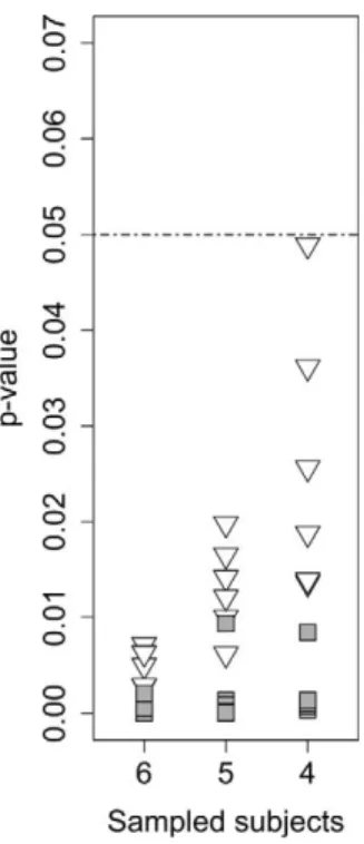
Thereafter, we compared the power of the two methods by resampling the original dataset. We randomly chose 6, 5, and 4 subjects of the original dataset and tested the hypothesisH0:b1down¼b1up with
both GLMM and PAOM (we used the LR test with GLMM). For each sample width, we repeated the analysis with six different combinations of subjects. As
shown in Figure 1, we could always reject the null
hypothesis. Thep-values were on average smaller with
GLMM than with PAOM. In this example, we performed more analyses than usually expected in a research article in order to illustrate different possibil-ities and potential pitfalls of GLMM.
Example 2: Johnston et al., 2008
Here we applied the two models on a dataset from Johnston et al. (2008), with permission of the
corre-sponding author. This paper showed that adaptation to an invisible flicker reduces the perceived duration of a
subsequently viewed stimulus (Ibid., experiment 1, pp.
2–4). We chose this dataset because the analysis performed in the original article showed a difference in the PSE between the two conditions. Each experi-ment consisted of an invisible flickering and control condition (140 trials per condition). The duration of the standard stimulus was fixed at 500 ms. Five subjects were tested.
We first applied the PAOM, and tested for a
difference between conditions with a paired t-test.
The difference in slope was not significant (t¼1.88,df¼
4, p¼0.13), whereas the difference in PSE was highly
significant (t ¼8.83, df¼4, p , 0.001). The average
difference was 33 ms. Then we applied the GLMM (probitlink function) on the same data set. The model was the following:
Y*ij¼g0þui0þxijðg1þu1iÞ þdijh2þ ðxijdijÞg3; ð13Þ where Y*ij is the latent variable, xij is the stimulus
duration,dijis the dummy variable for the experimental
condition (either 1 or 0),xijdijis the interaction between
the stimulus duration and the dummy variable, g0, . . ., Figure 1. Comparison of GLMM and PAOM by re-sampling method. We resampled the dataset from the article: Moscatelli and Lacquaniti (2011). We randomly chose six, five, and four subjects of the original dataset and tested the hypothesis
H0:b1down¼b1up with GLMM (filled squares) and PAOM (blank
triangles). The x-axis labels the number of subjects in each sample and the y-axis the corresponding p-value. For each sample width, we repeated the analysis with six combinations of subjects.
g3 are the fixed-effects coefficients, and u0i, u1i are the
random-effect parameters. As in the previous example, we included three random-effects parameters (the random intercept, the random slope and their correla-tion).Table 5 reports the estimate and standard error of the fixed-effect parameters. The significance of each parameter of the model was assessed by means of the Wald statistics.
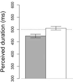
We thereby estimated the PSE and its standard
deviation with the Delta method (see Figure 2). The
estimates of the PSE were 47367 ms (mean6SD) in
Invisible Flicker condition and 505 6 7ms in the
Control condition. The difference between the two estimated values of PSE was 32 ms. We further evaluated the PSE with the bootstrap method (sampled
datasets B ¼ 600). The PSE was 473 ms (95%
confidence interval: 458-490 ms) in Invisible Flicker condition and 505 ms (95% confidence interval: 491-523 ms) in the Control condition. Crucially, the two confidence intervals estimated with the bootstrap method do not overlap.
The estimates of the PSE with the GLMM (using either the Delta or the bootstrap method) are close to the estimates with the PAOM, which are 475 and 508 ms respectively for Invisible Flicker and Control
condition (compare, for instance,Figure 2 with figure
1.B of the original article).
In conclusion, the PAOM and the GLMM consis-tently showed that the PSE was significantly shorter in the Invisible Flicker than in the Control condition.
Simulated data
We further tested the GLMM and PAOM on simulated data. With respect to the GLMM, we focused on fixed effects in the following simulations.
In order to get plausible values, we based our first set on a published article (Moscatelli, Polito, &
Lacqua-niti, 2011). We randomly sampled eight subjects from
the original dataset, in order to generate clustered data. Each of these subjects has been tested with nine possible values of a continuous predictor and 40 repetitions for each value, corresponding to a total number of 360 dichotomous responses per subject. We appropriately modified the initial data in order to set the PSE to a specific value, as follows. First, we fitted
the responses of each subject with a probit model so as
to estimate the parameters b0i and b1i. We then
centered each fitted model on the average of the continuous predictor, by choosing an appropriately shifted value of the intercept:
b*0i ¼ xb1i ð14Þ
In Equation 14, b*0i is the shifted intercept, x is the average value of the continuous predictor (equal to
800) and b1i is the fitted slope of the model. According
toEquation 2, the PSEi of each ‘‘shifted’’ model was:
PSEi ¼
b*0i b1i
¼x¼800 ð15Þ
Using the estimates b*0i and b1i, responses Yij were
randomly generated from a binomial (nij,pˆij) ; whereiis
the subject, j is the stimulus level, and pij ¼ U(b*0i þ b1ixij). We used the R function rbinom to generate
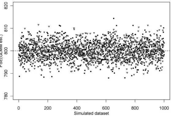
random numbers from the binomial distribution. The simulated data set consists of the set of counts along with their associated predictors, sample sizes and subject labels. The procedure was repeated 1,000 times, resulting in 1,000 randomly generated data sets. Each sampled dataset was then fitted with a GLMM (random intercept and slope) and a PAOM.
We first focused on the estimate of the PSE. In each dataset we estimated the PSE and its 95% confidence interval (CI; for the GLMM, CI was obtained by means of the Delta method, reducing the computa-tional load of the simulation). If both GLMM and PAOM were unbiased, we would expect the grand Parameter Estimate Standard error zvalue Pr(.jzj) g0(Intercept) 4.61845 0.65614 7.039 ,0.0001 g1(Duration) 0.00914 0.00137 6.688 ,0.0001 g2(Control Condition) 1.14258 0.409575 2.790 0.00528 g3(Interaction) 0.00180 0.00811 2.222 0.02631
Table 5. Fixed effects parameters of the GLMM (Example 2).
Figure 2. The PSE estimated with the Delta method. We re-analyzed the dataset from Johnston et al. (2008),‘‘Visually-based temporal distortion in dyslexia’’(with permission of Johnston, A., & Bruno, A.). The bar plot shows the estimated PSE in Flickering condition (in grey) and Control condition (in white). Vertical error bars show theSD. The dataset has been fitted with GLMM; the PSE and the SD were estimated with the Delta method.
mean of each model to be close to 800. We also would expect that the theoretical value of the PSE (800) fell within the CI in 95% of the samples. According to PAOM, the grand mean of the PSE was 799.97. We
performed a one-sample t-test for each simulated
experiment. In each t-test, the alternative hypothesis stated that the true value of the PSE was different from 800. Consistently with the expectation, we were unable to reject the null hypothesis in 49/1,000 samples (with a
significance-level a equal to 0.05). According to
GLMM, the grand mean of the PSE was 799.95. The 95% CIs did not include the theoretical value of the PSE (800) in 49/1,000 samples. Thus, the two methods resulted to be unbiased, and Type I Errors of the PSE were within the confidence level of 0.05.
In order to simulate an experimental effect, we added
a fixed value d to the slope of the probit model. For
each subject and stimulus level, we sampled the responses from a binomial distribution, where the specific probability of the outcome was determined using the following equation:
U1 PðYij ¼1Þ
¼b*0iþb1ixijþb2idijþdðxijdÞ ð16Þ
InEquation 16,dijis a dummy variable (dij¼1 in one
half of the observations),b2i¼ [800 (b1iþd)]b*0i,
and d accounts for a simulated experimental effect.
According to this equation, PSE¼800 for bothdij¼1
anddij¼0, while the difference in slope betweendij¼1
anddij¼0 is equal tod(actually,dis a parameter of the
model, just as b0i, . . ., b02. We used this notation to
highlight that this specific parameter accounts for a
simulated difference between experimental conditions).
Using this algorithm, we first checked the two models
for Type I Errors. With respect tod, the hypothesisH0
states that the parameter is not significantly different
from 0, thus we setd¼0 inEquation 16and simulated
1,000 data sets. In this case, we simulated 720 trials per subject (360 trials in each experimental condition, with
dij¼1 or dij¼0). With a confidence level of 0.05, we
would expectd to be not significantly different from 0
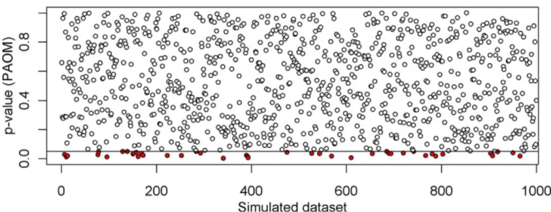
in less than 5% of the samples. We tested the parameter by means of the Wald statistics. The parameter was significantly different from 0 in 42/1,000 samples with
PAOM (Figure 3) and 38/1,000 samples with GLMM
(Figure 4). Furthermore, according to the two methods,
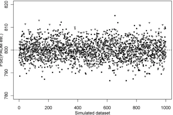
the two estimates of the PSE were unbiased (Figures 5
and6) and the PSE was significantly different from 800
in less than 5% of the samples.
Finally, we assessed the power of the two models by setting d .0. We always chose plausible values of the parameter (according to our original data set). In
different simulations, d was 0.0005, 0.001, 0.002 and
0.0026. According to PAOM, the parameter was significantly different from zero respectively in 210/ 1,000, 593/1,000, 996/1,000 and 1,000/1,000 samples. According to GLMM, the parameter was significantly different from zero respectively in 283/1,000, 795/1,000, 1,000/1,000 and 1,000/1,000 samples. As shown in
Figure 7, the GLMM has a higher power than PAOM
(0.0005.d.0.002) while Type I Errors are similar (d
¼0).
Discussion
Most psychophysical studies make inferences on the whole population by means of a two-level analysis (PAOM). This two-level analysis has several limits: it discards the subject-specific variability in the second step, it has a lower statistical power, and it does not allow assessing the overall goodness of fit easily. Generalized Linear Mixed Models (GLMMs) are a viable alternative to such two-level analysis. Here we compared the performance of GLMMs and PAOMs in psychophysics, using examples from the psychophysics of time perception. We briefly discussed several options for statistical inference on the parameters of the GLMM, such as the LR test, the AIC and the Wald statistics. None of these options apply to the estimate of the PSE. Therefore, we proposed to estimate the PSE Figure 3. Type I errors with PAOM. In each dataset, we tested the hypothesisH0:d¼0, wheredis the difference in slope betweenD¼1
and its uncertainty within the GLMM framework by means of the Delta and Bootstrap methods. The Delta method provides a confidence interval for the param-eter of interest. It approximates the paramparam-eter with a Gaussian distribution; the resulting confidence interval is therefore symmetric around the estimated parameter (Equation 11). The Delta method is computationally fast, and may provide a rapid estimate of the variability of the parameter. However, the normality assumption may not apply: the interval of the PSE can be skewed, and thus assuming a symmetric interval may lead to biases in the individual tail-coverage probabilities. Alternatively, the bootstrap method does not require
any a priori assumption about the interval of the PSE. It is not straightforward to decide a priori the number of replications (B) in bootstrap methods – this varies from case to case, depending also on the variability of the responses and on the size of the data set. Here, we increased progressively the size of B; for a given B we replicated 20 times the procedure, and empirically chose a size of B that guaranteed stable results between one replication and the other. As shown in
Supplementary T S1, in Example 1, the estimate of PSE and 95% CI is similar for a further increase of B. Both the bootstrap and the delta methods may underestimate the variability of the PSE in case of Figure 4. Type I errors with GLMM. We tested in each dataset the hypothesisH0:d¼0, wheredis the difference in slope betweenD¼1
andD¼0. We set the true value ofdequal to 0. They-axis shows thepvalue (Waldz) in each sample. In redp,0.05.
Figure 5. Simulated data; values of the PSE estimated with PAOM. We simulated 1,000 datasets according toEquation 18. The Figure shows the estimated PSE forD¼1 (white) andD¼0 (black). In both conditions, the theoretical value of the PSE was equal to 800 (dotted line).
overdispersion, however as we will illustrate below, it is possible to account for overdispersion in GLMM with different methods.
Next, we compared the PAOM and GLMM on real and simulated data. Overall, we found that the estimated values of the PSE and of the slope were similar between the two models. In simulated data sets, we found that Type I errors were within the confidence
level (p¼0.05) in both the PAOM and the GLMM. In
these simulations, we computed p-values of the d
parameter by means of the z Wald statistics, whereas in Example 1 and Example 2 we performed statistical inference by means of LR test and model comparison.
On real data, the z Wald statistics is unreliable if overdispersion occurs; this is not the case with simulated data, where the programmer can control the sources of variability. According to previous studies, Type I error rate in lme4 depends on both the number of clusters, repetitions and within-cluster correlations (Austin, 2010; Zhang et al., 2011). Austin
(2010) found that the empirical type I error rates were
acceptable as long as the number of subjects and repetitions per subject were larger than five. Similarly,
Bolker et al. (2009) suggested the rule-of-thumb of
including more than five subjects or clusters for each random effects, and more than 10 samples per each Figure 6. Simulated data; values of the PSE estimated with GLMM. The Figure shows the estimated PSE forD¼1 (white) andD¼0 (black). In both conditions, the theoretical value of the PSE was equal to 800 (dotted line).
Figure 7. Comparison of the statistical power of the two models. Percentage ofdsignificantly different from zero with respect to the true values of the parameter. Gray circles are the estimatedp-values with PAOM, black triangles with GLMM.
level of the linear predictor. The power of the analysis depends on the sample size, the effect size, and its
source of variability, that is, the rate ofyesresponses (it
will affect the variance in a Binomial distribution), the overdispersions, and the heterogeneity between subjects or clusters. Checking previous studies in the literature may help in predicting the correct sample size to address a specific experimental question.
The GLMMs have several advantages compared with PAOMs. First, GLMMs have a higher statistical
power than PAOMs (Figure 7). Second, model
comparison is easier within the GLMM framework than within the PAOM. Also, GLMMs separately account for the variability within and between subjects, by means of fixed and random effects, respectively. Therefore, although the experimenter will usually focus on fixed effects, she/he may want to look at the random effects to study the heterogeneity between subjects.
Fitting GLMMs may be rather complex because the likelihood function does not have a closed form solution. The function can be approximated thorough different numerical methods (Agresti,2002, paragraph 12.6). In Examples 1 and 2, we used the Gauss-Hermite
quadrature. The approximation is aweightedsum that
evaluates the function at certainquadrature points. The
approximation improves as the number of quadrature
points increases; inlme4package it is possible to choose
the number of points. Alternatively, the likelihood function can be approximated using Monte Carlo Markov Chain (MCMC) methods. The R package
lme4 allows the MCMC method in Linear Mixed
Model (LMM; Pinheiro & Bates,2000), however, at the
time we wrote the article, this is not possible for GLMMs. The R package MCMCglmm (Hadfield,
2010) allows fitting GLMMs by means of MCMC
algorithms. This package follows a Bayesian approach, and therefore the researcher has to choose a prior distribution of the parameters of the model. The Gauss-Hermite and Monte Carlo integration methods provide likelihood approximations, and the parameter estimates converge to the ML estimates, as the quadrature points and the sample size increase. Alternatively, the penalized quasi-likelihood method (PQL) maximizes the quasi-likelihood rather than the likelihood function. The PQL may yield biased estimates with binary data (Goldstein & Rasbash,
1996); Agresti (2002) recommends using ML rather
than PQL methods. Finally, it is worth noting that the likelihood ratio test cannot be used with the PQL fitting, because the test requires the ML. All methods discussed above are implemented in several R packages
(for a comparison, see Bolker et al.,2009; Austin,2010;
Zhang et al.,2011). The R-based code that we used in
this article is available on our web site (http://
mixedpsychophysics.wordpress.com).
GLMMs and related models also apply to unbal-anced experimental designs, may account for over-dispersion, and may extend to the Bayesian framework (see below). Here, we illustrated GLMMs with a random intercept and with a random slope and correlated random intercept. Although rarely applied in psychophysics, unbalanced experimental designs can be also modeled in the mixed-model framework by
means of nested random effects and crossed random
effects (Bolker et al., 2009). Both types of random effects can be implemented in lme4.
An issue that we mentioned before is that of overdispersion. This may occur in GLMMs and in other statistical models assuming a binomial distribution of the data (such as, for example, the ordinarylogitandprobit GLM). In GLMMs, it is possible to include subjects-level random effects in order to account for
over-dispersion (Agresti, 2002). Other tips on GLMM and
over-dispersion are in Agresti (2002), Bolker et al. (2009),
and the related web site:www.glmm.wikidot.com.
In our examples, we modeled functions whose lower and upper asymptotes were respectively 0 and 1; however, in mixed model framework it is also possible to model functions with different asymptotes. This takes into account the guessing and lapsing behavior, which affect respectively the lower and the upper asymptote of the function. Guessing is particularly important in n-Alternative-Forced-Choice (n-AFC) paradigms, where the lower asymptote approaches the probability of success for a random choice. Brockhoff and M ¨uller (1997) proposed a mixed model accounting for guessing behavior in multiple forced choice
experiments. They introduced the parameter c that
accounts for the base-line probability. The probability
ofYes response is therefore:
PðYij ¼1Þ ¼cþ ð1cÞPðeij.uib0xijb1Þ ð17Þ Using the latent variable that we introduced in
Methods, we can write the model as:
PðYij ¼1Þ ¼cþ ð1cÞY* ð18Þ
Brockhoff and M ¨uller (1997) applied a quasi-likeli-hood method to estimate the parameters. Their model
was applied to experimental data in Williams et al. (2006).
Yssaad-Fesselier and Knoblauch (2006) applied a
Gen-eralized Nonlinear Mixed Model to model lapses in psychometric functions. In their article, authors modeled the repeated responses of a single subject in different experimental conditions. They assumed that lapses originate from a random process, unrelated to experi-mental variables. In their model, a single random-effect parameter accounts for lapsing: therefore the number of parameters does not increase with the number of conditions, ensuring the parsimony of the model. The issue of modeling lapses was further discussed on the R group of interest ‘‘R-mixed-models,’’ by K. Knoblauch
and D. Bates among others (see https://stat.ethz.ch/ mailman/listinfo/r-sig-mixed-models, third and fourth quarter 2010). In psychometrics, similar solutions have been suggested within the framework of the Item
Response Theory (Fox,2010). Models discussed above
are not linear, and therefore cannot be fitted with the
lme4-functionglmer.
In the linear mixed model, random effects estimates of the unit means are compromises or weighted averages between the biased-but-efficient grand mean and the unbiased-but-inefficient unit mean. Random Effects models fit naturally into a Bayesian paradigm. Similar to the Bayesian approach, a mixed model specifies the model in a hierarchical fashion, assuming that parameters are random. However, unlike the Bayesian approach, hyperparameters are estimated from the data, and just as in the Bayesian approach, one has to make a decision on some prior assumption. It is possible to apply GLMM within the Bayesian framework with the already cited MCMCglmm R-package or other software, such as WinBUGS/Open-BUGS or JAGS. R-packages BRugs and rjags interface WinBUGS and JAGS with R.
In this article we showed that, in the classical two-level model, a considerable amount of information is lost when making inference on the whole population. Therefore, we proposed to use the GLMM for statistical inference on the whole population. Obvious-ly, studying the whole population is not at odds with studying each single subject. The aim of the GLMM is to quantify the variability in behavior between subjects and to draw conclusions on the whole set of data. In conclusion, we believe that the GLMM may prove quite useful in psychophysics, especially when different individuals of the population are heterogeneous in the variance of their experimental results.
Acknowledgments
The work was supported by the Italian Health Ministry, the Italian University Ministry (PRIN project), the Italian Space Agency (DCMC and CRUSOE grants), and the European Commission (Collaborative Project no. 248587, ‘THE Hand Em-bodied’). We thank Dr. Marieke Rohde, Dr. Cesare Parise, Professor Marc Ernst, and the two anonymous reviewers for their comments and suggestions. One of the two reviewers provided us withFigure S2, and the R-code for generating it.
Commercial relationships: none.
Corresponding author: Alessandro Moscatelli. Email: [email protected].
Address: Department of Cognitive Neuroscience, University of Bielefeld, Bielefeld, Germany.
Footnotes
1 In other branches of medicine this parameter is
known as LD50 (see, for example, Faraggi, Izikson, & Reiser,2003; Kelly, 2001).
2
In other fields of neuroscience, two-level statistical models have been proposed to take the subject-specific variability into account; see, for example, Me´riaux, Roche, Dehaene-Lambertz, Thirion, & Poline, 2006.
3
In Equation 4 and 5, we labeled the within and
between-subjects sources of variability with the eijand
uierror terms. These two error terms do not appear in
Equation 3because it is an expression for the expected value. Alternatively, we could write the between-subjects variability as a random-effects parameter
multiplied for a random weight predictor Z: Y*ij¼b0i
þb1ixijþuiZiþeij. The random predictorZequals to 1
for subject i and 0 otherwise. In matrix notation:Y*¼
Xb þ Zu þ e. We assume that u has a normal
distribution with mean 0 and variancer2u. This second
notation has been also frequently used (Breslow &
Clayton, 1993; Agresti, 2002).
References
Agresti, A. (2002). Categorical data analysis(2nd ed.). Hoboken, NJ: John Wiley & Sons.
Akaike, H. (1973). Information theory and an exten-sion of maximum likelihood principle. In B. N. Petrov, & F. F. Cs ´aki, (Eds.), Proceedings of the 2nd International Symposium on Information Theory (pp. 267–281). Budapest, Hungary: Akade´miai Kiad ´o.
Austin, P. C. (2010). Estimating multilevel logistic regression models when the number of clusters is low: A comparison of different statistical software procedures. The International Journal of Biostatis-tics, 6(1), 16.
Baayen, R. H., Davidson, D. J., & Bates, D. M. (2008). Mixed-effects modeling with crossed random ef-fects for subjects and items.Journal of Memory and Language, 59, 390–412.
Bates, D., Maechler, M., & Bolker, B. (2011). lme4: Linear mixed-effects models using S4 classes. R package version 0.999375-39. http://cran.r-project. org/web/packages/lme4/index.html.
W., Poulsen, J. R., Stevens, M. H., et al. (2009). Generalized linear mixed models: A practical guide
for ecology and evolution. Trends in Ecology and
Evolution, 24(3), 127–135.
Breslow, N. E., & Clayton, D. G. (1993). Approximate inference in generalized linear mixed models. Journal of American Statistical Association, 88, 9– 25.
Brockhoff, P. M., & M ¨uller, H.-G. (1997). Random effect threshold models for dose-response relation-ships with repeated measurements.Journal of Royal Statistical Society B, 59(2), 431–446.
Casella, G., & Berger, R. L. (2002).Statistical inference (2nd ed.). Pacific Grove, CA: Duxbury Press. Cox, D. R. (1958). The regression analysis of binary
sequences. Journal of the Royal Statistical Society B, 20, 214–242.
DeCarlo, L. T. (1998). Signal detection theory and
generalized linear models. Psychological Methods,
3, 186–205.
DeCarlo, L. T. (2010). On the statistical and theoretical basis of signal detection theory and extensions: Unequal variance, random coefficient and mixture
models. Journal of Mathematical Psychology, 54,
304–313.
Dur ´an Pacheco, G., Hattendorf, J., Colford, J. M. Jr, M ¨ausezahl, D., & Smith, T. (2009). Performance of analytical methods for overdispersed counts in cluster randomized trials: Sample size, degree of
clustering and imbalance. Statistics in Medicine,
28(24), 2989–3011.
Efron, B., & Tibshirani, R. J. (1993).An introduction to the bootstrap. New York: Chapman & Hall. Efron, B. (1987). Better bootstrap confidence intervals
(with discussion). Journal of American Statistical Association, 82, 171–200.
Faraggi, D., Izikson, P., & Reiser, B. (2003). Confi-dence intervals for the 50 per cent response dose. Statistics in Medicine, 22(12), 1977–1988.
Foster, D. H., & Bischof, W. F. (1997). Bootstrap estimates of the statistical accuracy of thresholds
obtained from psychometric functions. Spatial
Vision, 11, 135–139.
Fox, J. P. (2010). Bayesian item response modeling:
Theory and applications. New York: Springer. Fr ¨und, I., Haenel, N. V., & Wichmann, F. A. (2011).
Inference for psychometric functions in the pres-ence of nonstationary behavior. Journal of Vision,
11(6):16, 1–19, http://www.journalofvision.org/
content/11/6/16, doi:10.1167/11.6.16. [PubMed]
[Article]
Goldstein, H., & Rasbash, J. (1996). Improved approximations for multilevel models with binary responses. Journal of the Royal Statistical Society A, 159, 505–513.
Hadfield, J. D. (2010). MCMC methods for multi-response generalized linear mixed models: The
MCMCglmm R package. Journal of Statistical
Software, 33(2), 1–22.
Hoffman, L., & Rovine, M. J. (2007). Multilevel models for the experimental psychologist: Founda-tions and illustrative examples. Behavior Research Methods, 39(1), 101–117.
Johnston, A., Bruno, A., Watanabe, J., Quansah, B., Patel, N., Dakin, S., et al. (2008). Visually-based
temporal distortion in dyslexia. Vision Research,
48(17), 1852–1858.
Kelly, G. (2001). The median lethal dose—design and estimation.The Statistician, 50(1), 41–50.
Klein, S. A. (2001). Measuring, estimating, and understanding the psychometric function: A com-mentary. Perception & Psychophysics, 63(8), 1421– 145.
Knoblauch, K., & Maloney, L. T. (2012). Modeling
psychophysical data in R. New York: Springer. Kuss, M., J ¨akel, F., & Wichmann, F. A. (2005).
Bayesian inference for psychometric functions.
Journal of Vision, 5(5):8, 478–492, http://www.
journalofvision.org/content/5/5/8, doi:10.1167/5.5. 8. [PubMed] [Article]
Maloney, L. T. (1990). Confidence intervals for the parameters of psychometric functions.Perception & Psychophysics, 47, 127–134.
Me´riaux, S., Roche, A., Dehaene-Lambertz, G., Thirion, B., & Poline, J. B. (2006). Combined permutation test and mixed-effect model for group
average analysis in fMRI. Human Brain Mapping,
27(5), 402–410.
Mooney, C. Z., & Duval, R. D. (1993). Bootstrapping: A non-parametric approach to statistical inference. Newbury Park CA: Sage.
Morrone, M. C., Ross, J., & Burr, D. (2005). Saccadic eye movements cause compression of time as well as space. Nature Neuroscience, 8(7), 950–954. Moscatelli, A., & Lacquaniti, F. (2011). The weight of
time: Gravitational force enhances discrimination of visual motion duration. Journal of Vision, 11(4):
5, 1–17, http://www.journalofvision.org/content/
11/4/5, doi:10.1167/11.4.5. [PubMed] [Article]
Moscatelli, A., Polito, L., & Lacquaniti, F. (2011). Time perception of action photographs is more precise than that of still photographs.Experimental Brain Research, 210(1), 25–32.
Pariyadath, V., & Eagleman, D. (2007). The effect of
predictability on subjective duration. PLoS One,
2(11), e1264, doi:10.1371/journal.pone.0001264. Pinheiro, J. C., & Bates, D. M. (2000). Mixed-effects
models in S and S-PLUS. New York: Springer-Verlag.
Quene´, H., & van den Bergh, H. (2008). Example of mixed-effects modeling with crossed random effects
and with binomial data. Journal of Memory and
Language, 59, 413–425.
R Development Core Team. (2012). R: A language and environment for statistical computing. R Founda-tion for Statistical Computing, Vienna, Austria, http://www.R-project.org/.
Rasch, G. (1961). On general laws and the meaning of measurement in psychology. In J. Neyman & C. A. Berkeley (Eds.),Proceedings of the Fourth Berkeley Symposium on Mathematics, Statistics, and Proba-bility, Volume 4: Contributions to Biology and
Problems of Medicine (pp. 321–333). Berkeley,
CA: University of California Press.
Rouder, J. N., Lu, J., Sun, D., Speckman, P., Morey, R., & Naveh-Benjamin, M. (2007). Signal detection models with random participant and item effects. Psychometrika, 72, 621–642.
Stine, R. (1990). An introduction to bootstrap meth-ods. In J. Fox, & J. S. Long (Eds.),Modern methods of data analysis(pp. 325–373). Newbury Park, CA: Sage.
Treutwein, B. (1995). Adaptive psychophysical proce-dures. Vision Research, 35(17), 2503–22.
Wichmann, F. A., & Hill, N. J. (2001a). The psychometric function. I. Fitting, sampling and goodness-of-fit. Perception & Psychophysics, 63(8), 1293–1313.
Wichmann, F. A., & Hill, N. J. (2001b). The psychometric function. II. Bootstrap-based confi-dence intervals and sampling. Perception & Psy-chophysics, 63(8), 1314–1329.
Williams, J., Ramaswamy, D., & Oulhaj, A. (2006). 10 Hz flicker improves recognition memory in older
people. BMC Neuroscience, 5, 7–21.
Yssaad-Fesselier, R., & Knoblauch, K. (2006).
Mod-eling psychometric functions in R. Behavior
Re-search Methods, 38(1), 28–41.
Zhang, H., Lu, N., Feng, C., Thurston, S. W., Xia, Y., Zhu, L., et al. (2011). On fitting generalized linear mixed-effects models for binary responses using different statistical packages.Statistics in Medicine.
Epub ahead of print. Internet site: http://
onlinelibrary.wiley.com/doi/10.1002/sim.4265/full (Accessed October 9, 2012).
Appendix A
Here we focus on the difference in the error term in
GLM and GLMM. We start from the GLM withprobit
link function (as in Equation 1): U1 PðYij ¼1Þ
¼b0iþb1ixij ðA1Þ
A latent dependent variable Y*ij, with normally
distributed errors, motivates the probit regression model. It is assumed that Y*
ij is a continuous variable,
and that it is a linear function of the test stimulus xij
(since the reference stimulus has a constant value):
Y*ij ¼b0iþb1ixijþeij ðA2Þ
We assume that Y*ij is related to the observed
dichotomous dependent variable Yij¼
1 if Y*
ij.0
0 if Y*ij 0 ðA3Þ
(
We also assume that the error termeijhas a standard
normal distribution. Therefore:
PðYij ¼1Þ ¼PðY*ij.0Þ ¼Pðb0iþxijb1iþeij.0Þ ¼
¼Pðeij.b0ixijb1iÞ ¼Uðb0iþxijb1iÞ
PðYij¼0Þ ¼PðY*ij0Þ ¼Pðb0iþxijb1iþeij 0Þ ¼
¼Pðeij b0ixijb1iÞ ¼1Uðb0iþxijb1iÞ
ðA4Þ
The inverse function of U() is the probit function, as
shown in Equation A1. Note that the latent approach
does not necessarily require the assumption of unitary
variance. In fact, in Equation A2, if eij instead of a
standard Gaussian, has a Gaussian distribution with 0
mean and variancer2, we can easily deriveEquation A4:
PðYij ¼1Þ ¼PðY*ij.0Þ ¼Pðb0iþxijb1iþeij.0Þ ¼P b0i r2þxij b1i r2 þ eij r2.0 ¼P eij r2. b0i r2xij b1i r2 ¼U b0i r2þxij b1i r2
Assuming unit variance makes distributions easier to handle, and makes parameters easier to interpret; the nonuniqueness of parameterization does not compro-mise the identifiability. This is the classical psycho-physical model for the single subject.
The GLMM is an extension of GLM that allows the analysis of repeated measures from several subjects. We recall from Equation 5:
U1 PðYij ¼1Þ
The error term differs between the ordinary GLM and the GLMM. In the GLM, we introduced the latent variableY*
ij and the normally distributed error termeij.
Within the mixed model framework,Y*
ij becomes:
Y*ij ¼b0þb1xijþmij ðA6Þ
The error term mij is the sum of two components ui
andeij, such that:
vij¼uiþeij ui;Nð0;r2uÞ eij;Nð0;r2eÞ
ðA7Þ
The error-term eij represents the variability within
subjects and the error-term ui the variability between
subjects. The model implies that the correlation
between two error terms for the same individual i is a constant qgiven by:
q¼Corrðvim;vinÞ ¼ r2 u r2 uþr2e ðA8Þ
Where vim and vin are error-terms from different
trials and within the same subject. While error terms within the same subject are positively correlated (Equation A8), they are independently conditional on
the random parameter ui. The higher r2u, the higher is
the correlation between the error terms of the same
subject. According to the model (Equation A5andA6),
vim and vin are independent only for a degenerate