Inaugural-Dissertation
zur Erlangung des Grades eines
Doktors der Wirtschaftswissenschaften (Dr. rer. pol.)
des Fachbereichs
Wirtschaftswissenschaften, Wirtschaftsinformatik und Wirtschaftsrecht der Universität Siegen
vorgelegt von
Guido Schultefrankenfeld aus Frankfurt am Main
Frankfurt am Main, den 24.04.2013
Vorsitzender: Prof. Dr. Sebastian G. Kessing, Universität Siegen
Erstgutachter: Prof. Dr. Günter W. Beck, Universität Siegen
Zweitgutachter: Prof. Dr. Peter Tillmann, Universität Gießen
Die mündliche Prüfung fand am 02.04.2014 statt.
Introduction 1
1 How Informative Are Central Bank Assessments of Macroeconomic Risks? 9
1.1 Introduction . . . 10
1.2 An Overview of Risk Forecasting . . . 12
1.3 Data . . . 18
1.3.1 Data Sources . . . 18
1.3.2 Summary Statistics . . . 21
1.3.3 Bias Tests . . . 23
1.4 Methodology . . . 24
1.5 Analysis of Risk Assessments . . . 27
1.5.1 Quantitative Assessments . . . 27
1.5.2 Direction-of-Risk Assessments . . . 29
1.5.3 Summary of Empirical Results . . . 31
1.6 Reconsidering the Rationale for Risk Assessments . . . 31
1.7 Conclusion . . . 34
References . . . 36
A.1 Central Bank Statements on Risk Forecasting . . . 40
A.2 Data Details . . . 46
A.2.1 Bank of England . . . 46
A.2.2 Sveriges Riksbank . . . 48
2 What determines the Shape of Inflation Fan Charts? 50 2.1 Introduction . . . 51
2.2 Data . . . 53
2.2.1 Fan Chart Width and Skewness . . . 53
2.2.2 Individual and Aggregate Interest Rate Decisions . . . 55
2.3 Investigating Fan Chart Width and Skewness . . . 59
2.3.1 Two Options to Accomodate Minority Views . . . 59
2.3.2 Regression Models . . . 60
2.3.3 Results . . . 61
2.4 Accounting for Hawkish and Dovish Voting . . . 63
2.4.1 Individual Monetary Policy Stances . . . 63
2.4.2 Regression Models . . . 63
2.4.3 Results . . . 64
2.5 Conclusion . . . 67
References . . . 68
3 The Empirical (Ir)Relevance of the Interest Rate Assumption for Central Bank Forecasts 72 3.1 Introduction . . . 73
3.3.2 Synchronizing Market Expectations and Constant Rate Forecasts . . . 83
3.3.3 Effects of an Interest Rate Change on Inflation and Growth . . . 84
3.4 Properties of the Forecasts . . . 87
3.5 Testing for Equal Predictive Accuracy . . . 89
3.6 Conclusion . . . 91
References . . . 93
A.1 Plots and Results Tables . . . 97
A.2 Central Bank Statements on Forecast Conditioning Assumptions . . . 112
4 Forecast Uncertainty and the Bank of England’s Interest Rate Decisions 118 4.1 Introduction . . . 119
4.2 Data . . . 121
4.2.1 Interest Rate Decisions . . . 121
4.2.2 Forecast Inflation and Forecast Real Output Growth . . . 123
4.2.3 Forecast Inflation Uncertainty and Forecast Real Output Growth Un-certainty . . . 124
4.2.4 Forecast Inflation Risk and Forecast Real Output Growth Risk . . . . 126
4.3 Forecast-based Interest Rate Rules augmented by Forecast Uncertainty . . . . 127
4.3.1 The Regression Model . . . 127
4.3.2 Estimation Results . . . 129
4.4 Accounting for Asymmetric Uncertainty Forecasts . . . 133
4.4.1 The Regression Model . . . 133
4.4.2 Estimation Results . . . 134
4.4.3 Remarks on Robustness Checks . . . 138
4.5 Forecast Uncertainty derived from the Survey of External Forecasters . . . . 140
4.5.1 Data Description . . . 140 4.5.2 Estimation Results . . . 142 4.6 Conclusion . . . 143 References . . . 145 Conclusion 149 V
1.1 Central bank assessments of macroeconomic balances of risks . . . 15
1.2 Summary statistics for forecast data of the Bank of England and the Sveriges Riksbank . . . 21
1.3 Tests for bias of forecast mean and forecast variance . . . 24
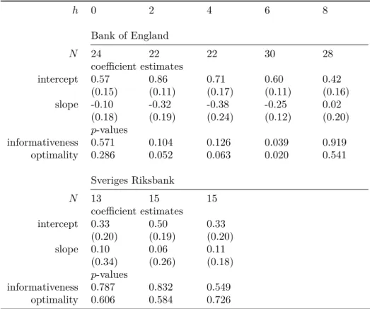
1.4 Panel-based tests for bias, informativeness and optimality of quantitative risk forecasts of the Bank of England and the Sveriges Riksbank . . . 29
1.5 Tests for informativeness and optimality of direction-of-risk forecasts of the Bank of England and the Sveriges Riksbank . . . 30
1.6 Publications of risk assessments by central banks . . . 43
1.7 Pearson mode skewness of forecast densities of the Bank of England . . . 47
1.8 Pearson mode skewness of forecast densities of the Sveriges Riksbank . . . 49
2.1 Effects of monetary policy committee dissent on fan charts width . . . 62
2.2 Effects of monetary policy committee dissent on fan chart skewness . . . 63
2.3 Effects of hawkish and dovish monetary policy meetings on fan chart width . 65 2.4 Effects of hawkish and dovish monetary policy meetings on fan chart skewness 66 2.5 Timing of central banks’ interest rate announcements and inflation report pub-lications . . . 70
2.6 Typecasting of monetary policy committee members by measuring average dissent 71 3.1 Interest rate assumptions in central banks . . . 77
3.2 Average R2 for different estimation approaches . . . 99
3.3 Correlations of interest rate forecasts . . . 101
3.4 Correlations of inflation forecasts . . . 102
3.5 Correlations of GDP growth forecasts . . . 103
3.6 Root mean squared errors of interest rate mean forecasts . . . 104
3.7 Root mean squared errors and mean logarithmic scores of inflation mean and density forecasts . . . 105
3.8 Root mean squared errors and mean logarithmic scores of GDP growth mean and density forecasts . . . 106
3.9 Test results for equal predictive accuracy of interest rate mean forecasts based on squared errors . . . 107
3.10 Test results for equal predictive accuracy of inflation mean forecasts based on squared errors . . . 108
3.11 Test results for equal predictive accuracy of GDP growth mean forecasts based on squared errors . . . 109
based on logarithmic scores . . . 111
4.1 Overview on the Bank of England’s number of forecast upward, balanced and downward risks . . . 127 4.2 Selected OLS estimation results for equation (4.7) - Accounting for forecast
uncertainty . . . 132 4.3 Selected OLS estimation results for equation (4.9) - Accounting for forecast risk 136 4.4 Selected OLS estimation results for equation (4.10) - Separating the direction
of forecast risk . . . 139 4.5 OLS estimation results for data from Survey of External Forecasters . . . 143
1.1 Two of the Bank of England’s density forecasts for inflation . . . 13 1.2 Scatter plots for the Bank of England and the Sveriges Riksbank . . . 20 1.3 Plots of the differences between the mean forecast and the mode forecast for
the Bank of England and the Sveriges Riksbank . . . 22
2.1 Disagreement in the Bank of England’s monthly interest rate decisions . . . . 55 2.2 Disagreement in central banks’ interest rate decisions . . . 58
3.1 Response paths for inflation . . . 97 3.2 Response paths for real GDP growth . . . 98 3.3 Forecasts by the BoE and corresponding realizations for the policy rate,
infla-tion, and GDP growth from 2004Q2 and 2008Q4, respectively . . . 100
4.1 Plots of Bank of England forecast data for inflation. . . 122 4.2 Plots of Bank of England forecast data for real output growth. . . 125 4.3 Visualized marginal significance levels for coefficient estimates when varying
the forecast horizons in equation (4.7) . . . 131 4.4 Visualized marginal significance levels for coefficient estimates when varying
the forecast horizons in equation (4.9) . . . 135 4.5 Visualized marginal significance levels for coefficient estimates when varying
the forecast horizons in equation (4.10) . . . 137 4.6 Comparing Bank of England’s and the Survey of External Forecasters’ point
and uncertainty forecasts at the policy horizon. . . 141
I’ve just picked up a fault in the AE35 unit. It’s going to go 100% failure in 72 hours. [...] The 9000 series is [...], by any practical definition of the words, foolproof and incapable of error.
—HAL 9000 in Stanley Kubrick’s 2001: A Space Odyssey
The ultimate goal of today’s monetary policy makers around the world is to maintain price stability. Modern central banks mostly have refined this goal to keeping inflation on a well-defined target value, or, in case of deviation, bringing inflation back to target. Often, monetary policy makers have the additional pursuit of stabilizing output around potential output. To control these target variables inflation and output growth, a central bank sets the level of its control variable, which usually is some short-term interest rate. Lags in monetary policy transmission, however, complicate the issue, such that a change in interest rates affects inflation and output growth with considerable delay only. Thus, to set interest rates properly, central banks typically consider future values of inflation and output growth when casting the level of the key interest rate. Since these future values are unknown, central banks engage in forecasting to make informed monetary policy decisions in a best possible way.
Different from the science fiction example quoted above, forecasts in the real world are inherently subject to uncertainty. While in earlier times, central banks had a clear emphasis on point forecasts, they have by now recognized that assessments of future uncertainties and risks to the economy are valuable information in their own rights. Today, monetary policy makers employ human capital, computer power and sophisticated models extensively to cope with keeping the standard of publishing forecasts for inflation and output growth in company of an explicit quantification of the respective forecast uncertainties and their potential asymmetries, mostly by publishing entire density forecasts. Moreover, central bankers have contributed to the public understanding of matters by visualizing possible future inflation and output growth values and their uncertainty ranges in form of the well-known fan charts.
A number of questions can come up when considering the intricate and also delicate task for a central bank to making statements concerning likely future developments of the economy. Specifically, it is important to understand why and how central banks communicate
their forecasts, and what these central bank forecasts ought to convey besides pure figures. Therefore this thesis aims at providing answers to four specific questions related to the infor-mational and political dimensions of density forecasts and fan charts. This is accomplished by questioning, first, the information content of macroeconomic risk forecasts, second, the construction principles of fan charts, third, the implication of conditioning assumptions for forecast accuracy of point and density forecasts and, fourth, the overall usability of uncertainty and risks forecasts for monetary policy decisions.
Chapter one deals with the information contained in macroeconomic risk forecasts, which are hardly studied in the literature, given that central banks have only since fairly recently been engaged in the quantification of future asymmetries of forecast uncertainty. Many central banks have started providing assessments of the uncertainty surrounding point forecasts and, in addition, a large share of these banks also issues statements about the probability of future outturns lying above or below the point forecasts. Hence, these monetary policy makers are explicit about the asymmetry of the forecast density.
When studying central bank statements, the term ‘risk’ generally appears, usually in form of phrases like ‘the overall risks’, ‘the balance of risks’, or simply ‘the risks’ to a certain variable. A typical example is a statement as made by the Board of Governors of the Federal Reserve System (2008, p. 41), saying that “Most participants viewed the risks to their projections for GDP growth as weighted to the downside.” Such statements thus apparently often refer to the entire set of single risks that have been identified and weighted by their perceived probabilities of materialization as well as their potential impact, while a single risk is usually understood as a possible future event whose occurrence would lead to outturns markedly different from the point forecasts. Hence, statements as shown above are supposed to contain information about the asymmetry of the forecast density.
Forecasting a phenomenon related to third moments, however, is an extremely chal-lenging task, which might be illustrated by the fact that many central banks simply base their assessment of forecast uncertainty, i.e. a phenomenon related to second moments and there-fore generally easier to assess, on past there-forecast errors, see for instance Deutsche Bundesbank (2010, pp. 34-36) for an overview. This is due to the lack of models which can accomplish this task, as explained by Wallis (1989). If forecasting uncertainty appropriately is already difficult, and central banks nonetheless engage in risk forecasting despite the difficulties en-countered, it is important to find out how successful these risk forecasts are and whether there is a systematic connection between risk forecasts and mode forecast errors.
This question is investigated using risk forecasts for inflation published by the Bank of England and the Sveriges Riksbank. If there is a systematic connection, given the point forecast is a mode forecast, upside [downside] risks should on average be followed by outturns that are greater [less] than the point forecasts. Moreover, the magnitude of the mode forecast error should on average correspond to the magnitude of the suitably defined forecast risk. If this is the case, the risk forecasts can be considered optimal, or rather, partially optimal in the sense of Diebold and Lopez (1996). If there is no systematic connection, i.e. if the risk forecasts do not help to predict the mode forecast errors, the risk forecasts are uninformative. It turns out that there is considerable evidence against the optimality of risk forecasts, at least for the Bank of England. For both the Bank of England and the Sveriges Riksbank, no robust evidence is found that risk forecasts have the intended information content. Hence, it seems that there is no systematic connection between risk forecasts and mode forecast errors.
Nonetheless, central banks continue to cast assessments of risks into density forecasts, and chapter two investigates further the reasons why. Results from density forecasting are often depicted as graphs of the central projection and potentially asymmetric uncertainty intervals surrounding this projection, known as fan charts. While potentially asymmetric fan charts are a well established device for monetary policy makers to communicate a baseline and its uncertainties, there exists an oddity regarding their construction. Usually, central bank fan charts are not generated by a model. Blix and Sellin (1999, pp.2-3) describe for the Sveriges Riksbank that “The traditional statistical approach to producing uncertainty intervals would involve [...] constructing a model intended for inflation forecasts. [...] The Riksbank, however, does not use the approach [...].” It is documented, for instance by Britton, Fisher, and Whitley (1998, p.32) for the Bank of England, that fan charts are rather the result of a forecasting process where the “central tendency for inflation [...], the degree of uncertainty [...] and the balance of risks” are to be evaluated. Further examples of central banks that follow this practice include the Magyar Nemzeti Bank, the Banco Central do Brazil and the Banco Central de Chile.
If central bank fan charts are not resulting from a model, the question arises how width and skewness of these graphical devices are set. More generally speaking, what determines the shape of central bank fan charts? Reasons for macroeconomic risk forecasting, which is closely related to skewed densities and asymmetric fan charts, are collected by Knüppel and Schultefrankenfeld (2012) and include non-linearities, frozen-forecast issues, biases in recent forecast errors, expert expectations about future asymmetries of shocks or simply from central bank communication strategies.
An important reason for risk forecasting that virtually summarizes the aforementioned ones is disagreement in decision-making. Disagreement in decision-making within institutions, in particular in the form of disagreement and dissenting views in monetary policy committees, plays a prominent role, since forecasting and monetary policy decisions are usually the concern of several decision-makers in a decision-making body of a central bank. In committees such as the Monetary Policy Committee of the Bank of England, the Policy Board of the Bank of Japan, the Federal Open Market Committee at the Federal Reserve System and the Governing Council of the European Central Bank, several members vote on an interest rate proposal made by the chairman to raise, maintain or lower the key interest rate. If at the end of the voting procedure a proposal has attained the majority of the member votes, the aggregate interest rate decision is achieved. In a second round, the committee then has usually to agree on an aggregate inflation projection that consistent with this interest rate decision.
Typically, committee members form their interest vote on the basis that inflation in two years ahead has to be on target. If there are minority views that do not agree with the interest rate decision, these minority voters probably do not agree with the aggregate projection, as they may consider future inflation unlikely to hit the target given the aggregate interest rate decision. If views of the decision-making body as a whole are represented by fan charts, then it seems reasonable that dissenting views on monetary policy have an effect on the shape of central bank inflation fan charts.
Although no individual inflation forecasts are available, the Bank of England, the Mag-yar Nemzeti Bank and the Sveriges Riksbank are the only central banks that make attributed interest rate voting records as well as the entire forecast densities published in their inflation reports available. Hence, the individual paths of interest rates for the committee members can
be determined. This dataset allows to investigate if there is a systematic connection between the degree of disagreement about monetary policy committee decisions on the level of the policy instrument and risks and uncertainties to forecasts of the target variable inflation, as published in the subsequent monetary policy reports. Disagreement is found to translate into wider fan charts in case of the Hungarian national bank. For the Bank of England and the Sveriges Riksbank, there is statistical evidence that disagreement on the level of interest rates can fairly well explain the skewness of forecast inflation fan charts. This prepares ground for the argument that dissenting views in monetary policy committees voting on central banks’ level of the policy instrument are a significant determinant of the shape of forecast inflation fan charts.
After having addressed the relationship between disagreement on interest rates and density forecasts, chapter three takes a different perspective and asks if certain assumptions about the future path of interest rates affect the predictive accuracy of mean and density forecasts of central banks. For the forecasts of variables central banks intend to control, the policy variable, i.e. the short-term interest rate set by the central bank, plays a special role. According to Galí (2011), in practice one can basically distinguish three approaches. Firstly, forecasts can be conditioned on a constant interest-rate assumption, such that the interest rate is assumed to remain at the level it had attained at the time the forecast was made. This so-called CIR approach was pursued, for example, by the ECB until 2006 and the Sveriges Riksbank until the end of 2005. Secondly, the expectations of market participants can serve as a conditioning assumption about the interest rate path. The so-called ME approach is current practice at, for example, the Bank of Japan and the ECB. Market expectations are usually derived from the term structure of interest rates. Finally, a central bank can issue unconditional forecasts for its target variables by using its own expectations about the interest rate path. The CBE approach, as it is called, has been adopted, for instance, by the Norges Bank, the Riksbank and the Federal Reserve System. The Fed’s December 2011 FOMC statement contributed to drawing the attention of economists to the topic of interest rate assumptions when announcing that “participants agreed that adding their projections of the target federal funds rate to the economic projections already provided in the SEP [Summary of Economic Projections] would help the public better understand the Committee’s monetary policy decisions”.
Among academics, there seems to be a clear ranking of the three approaches in terms of their suitability for central bank forecasts. Galí (2011), Svensson (2006) and Woodford (2005) advocate the approach of central bank expectations, i.e. prefer unconditional forecasts. Galí (2011) shows that it is possible to construct different forecasts conditional on one given nominal interest rate path, thus calling into question any conditioning assumptions about interest rates, and a similar point is raised by Woodford (2005). Overall, in the theoretical literature, it is evident that the CBE approach is supposed to yield the highest forecast accuracy. This property serves as one of the main reasons for preferring the CBE approach over conditional forecasts. For instance, Galí (2011, p.539) states that “it is not clear why the central bank would want to base its projections on a rule other than the actual rule it follows for, among other things, in that case the projections would also correspond to the best unconditional forecasts”. Svensson (2006) also resorts to the potential gains in forecast accuracy when advocating the CBE approach. The literature does not provide comparably clear ideas concerning the relative forecast accuracy of the ME approach with respect to the
CIR approach. However, it seems plausible that the ME approach should perform better unless the policy rate is best described by a random walk.
A large share of central banks, however, does not base its forecasts on its own interest rate expectations, probably also to circumvent potential communication issues. Goodhart (2009), for instance, finds that using the central bank’s expectations of the interest rate could be misunderstood as a commitment. Therefore, an interest rate path derived from market expectations is “a brilliant compromise” (Goodhart 2009, p. 94) between the potential lack of credibility of a constant rate assumption and the problems associated with publishing a path of future interest rates expected by the central bank. However, there are also central banks, for instance the Swiss National Bank, that use the constant interest rate assumption, whose merits are described in Goodhart (2001). Several empirical aspects related to interest rate assumptions are investigated in Andersson and Hofmann (2009), for instance that if a central bank is transparent and committed to maintaining price stability, the behavior of key variables like inflation expectations and long-term bond yields does not seem to be affected by the type of interest-rate assumption. In contrast to that, Winkelmann (2010) finds that using the CBE approach instead of the ME approach leads to better private-sector forecasts of longer-term interest rates.
The effects of the interest rate assumptions is assessed by testing for differences in forecast accuracy, since forecast accuracy is one the main reasons given in the academic literature for preferring the CBE approach. Moreover, forecast accuracy is related to central bank communication and the banks’ ability to steer market expectations for interest rates, inflation, and growth, and, thus, financial variables like bond yields, if the precision of central bank information varies with the conditioning assumption. Hence, forecast accuracy may also to detect if any of the three forecasting approaches yields improvements in monetary policy, such that central banks may better control macroeconomic volatility. To this extent, interest rate, inflation forecast and real GDP data from the Bank of England and the Banco Central do Brazil are exploited in order to assess the impact of the various interest rate assumptions on forecast accuracy. Results show that there is no significant difference in the predictive accuracy of competing forecast made conditional on different interest rate assumption. Thus, the theoretical ranking of the CBE, ME and CIR approaches cannot be confirmed empirically on the basis of data from the two central banks.
Finally, chapter four asks how central banks utilize information from their own forecasts of their target variables, in particular so from uncertainty and risk forecasts of these, when deciding on monetary policy. Monetary policy makers, such as the Bank of England, Sveriges Riksbank, Banco de Portugal, or Magyar Nemzeti Bank, to name but a few, publish entire probability distributions of the forecast variables inflation and output growth and thereby explicitly quantify forecast uncertainty. Forecasting entire densities is not an end in itself. If monetary policy decisions are made subject to economic prospects, it seems reasonable that uncertainty about these prospects may have an influence on the decisions.
Forecast-based rules encompass the lags of monetary policy transmission, and the fore-cast data are already conditioned on the relevant information set on future economic develop-ments, see Batini and Haldane (1999). Thus, forecast-based rules can be a fairly precise and yet compact tool for characterizing historical monetary policy decisions, as shown by Kuttner (2004) who evaluates forecast-based rules for New Zealand, Sweden, the United Kingdom, and the United States. Similarly, Goodhart (2005) presents estimates of a forecast-based Bank
of England’s Monetary Policy Committee reaction function and emphasizes the Committee’s high degree of forward-looking with respect to inflation. Besley, Meads, and Surico (2008) analyze the role of heterogeneity among the board members of the bank’s committee in a forecast-based rule setting. Gorter et al. (2008, 2009) provide evidence for the performance of interest rate rules for the European Central Bank, based on expectations data constructed from Consensus Economics forecasts. Orphanides and Wieland (2008) explain the Federal Open Market Committee decisions by its own projections for inflation and unemployment.
Studies in particular of Bhattacharjee and Holly (2010), Kim and Nelson (2006) and Martin and Milas (2005a, 2005b, 2006, 2009) have considered the impact of uncertainty on interest rate decisions and find either intensified or attenuated reactions. Yet, the uncertainty measures used in these studies do not reflect the measure of uncertainty that the institution under study was facing when making the monetary policy decision. To account for that lack, chapter four shows how to recover the exact forecast standard deviations for inflation and for output growth directly from the forecast densities which are published by the Bank of England between 1997Q4 and 2009Q4, following a recipe of Wallis (2004). These forecast standard deviations originally associated with the forecast location parameters reflect the genuine and thus relevant measure of uncertainty about future economic developments which the Monetary Policy Committee has available at the time the interest rate decision is made. Uncertainty measures are incorporated directly in forecast-based interest rate reaction functions in order to estimate the strength and the direction of the impact of forecast uncertainty on the Monetary Policy Committee’s interest rate responses to forecast deviations of inflation from target and output growth from long-run mean.
Since the Bank of England emphasizes its use of the two-piece normal distribution, potential asymmetries in forecast uncertainty have to be taken into consideration. Forecast uncertainty is asymmetric when an average of likely alternative outcomes for one variable is seen to exceed or to fall short of the central projection for that variable. The Monetary Policy Committee defines such a difference between mean and mode forecast as forecast risk to the central projection. Hence, to control for these risks, the exact forecast Pearson mode skewness for inflation and for output growth, is included into the regression models. Results show that forecast inflation uncertainty has a very strong and intensifying effect on interest rate reactions. In contrast, forecast output growth uncertainty has an attenuating effect on the interest rate decision response. Forecast upward risks to inflation contribute to the intensifying effect of forecast inflation uncertainty. Forecast risks for inflation have a direct effect on interest rate decisions, in particular when the central projection for inflation is close to target. Interestingly, the bank’s inhouse uncertainty and risk measures seem to be exhaustive, as insignificant results obtained from using direct uncertainty and risk measures constructed from the density forecasts of the bank’s Survey of External Forecasters show.
References
Andersson, M., Hofmann, B., October 2009. Gauging the effectiveness of quantitative forward guidance - Evidence from three inflation targeters. ECB Working Paper (1098).
Batini, N., Haldane, A. G., 1999. Monetary Policy Rules. The University of Chicago Press, Ch. ‘Forward-Looking Rules for Monetary Policy’, pp. 157–192.
Besley, T., Meads, N., Surico, P., 2008. Insiders versus Outsiders in Monetary Policymaking. American Economic Review: Papers and Proceedings 98 (2), 218–223.
Bhattacharjee, A., Holly, S., July 2010. Rational Partisan Theory, Uncertainty, and Spatial Voting: Evidence for the Bank of England’s MPC. Economics & Politics 22 (2), 151–179. Blix, M., Sellin, P., 1999. Inflation forecasts with uncertainty intervals. Sveriges Riksbank
Quarterly Review 2, 12–28.
Board of Governors of the Federal Reserve System, July 2008. Monetary policy report to the congress.
Britton, E., Fisher, P., Whitley, J., February 1998. Quarterly Bulletin. Bank of England, Ch. ‘The Inflation Report Projections: Understanding the Fan Charts’, pp. 30–37.
Deutsche Bundesbank, June 2010. Monthly report.
Diebold, F. X., Lopez, J. A., 1996. Forecast evaluation and combination. In: Maddala, G. S., Rao, C. R. (Eds.), Handbook of Statistics. Vol. 14. Elsevier, Ch. 8, pp. 241–268.
Galí, J., 2011. Are central banks’ projections meaningful? Journal of Monetary Economics 58, 537–550.
Goodhart, C., 2001. Monetary transmission lags and the formulation of the policy decision on interest rates. Federal Reserve Bank of St. Louis Review 83 (4), 165–182.
Goodhart, C., June 2009. The Interest Rate Conditioning Assumption. International Journal of Central Banking, 85–108.
Goodhart, C. A., 2005. The Monetary Policy Committee’s Reaction Function: An Exercise in Estimation. Topics in Macroeconomics 5 (1), Article 18.
Gorter, J., Jacobs, J., de Haan, J., 2008. Taylor Rules for the ECB using Expectations Data. Scandinavian Journal of Economics 110 (3), 473–488.
Gorter, J., Jacobs, J., de Haan, J., November 2009. Negative rates for the euro area? Central Banking 20 (2), 61–66.
Kim, C.-J., Nelson, C. R., 2006. Estimation of a forward-looking monetary policy rule: A time-varying parameter model using ex post data. Journal of Monetary Economics 53 (8), 1949–1966.
Knüppel, M., Schultefrankenfeld, G., September 2012. How informative are central bank assessments of macroeconomic risks? International Journal of Central Banking 8 (3), 87– 139.
Kuttner, K. N., July/August 2004. The Role of Policy Rules in Inflation Targeting. Federal Reserve Bank of St. Louis Review 86 (4), 89–111.
Martin, C., Milas, C., July 2005a. Uncertainty and Monetary Policy Rules in the United States. Keele Economic Research Papers (10).
Martin, C., Milas, C., July 2005b. Uncertainty and UK Monetary Policy. Keele Economic Research Papers (11).
Martin, C., Milas, C., June 2006. The Impact of Uncertainty on Monetary Policy Rules in the UK. Keele Economic Research Papers (9).
Martin, C., Milas, C., April 2009. Uncertainty and Monetary Policy Rules in the United States. Economic Inquiry 47 (2), 206–215.
Orphanides, A., Wieland, V., July/August 2008. Economic Projections and Rules of Thumb for Monetary Policy. Federal Reserve Bank of St. Louis Review 90 (4), 307–324.
Svensson, L. E. O., 2006. The Instrument-Rate Projection under Inflation Targeting: The Norwegian Example. Centre for European Policy Studies Working Paper (127).
Wallis, K. F., 1989. Macroeconomic Forecasting: A Survey. Economic Journal 99, 28–61. Wallis, K. F., 2004. An Assessment of Bank of England and National Institute Inflation
Forecast Uncertainties. National Institute Economic Review 189, 64–71.
Winkelmann, L., December 2010. The norges bank’s key rate projections and the news element of monetary policy: a wavelet based jump detection approach. SFB 649 Discussion Papers SFB649DP2010-062, Sonderforschungsbereich 649, Humboldt University, Berlin, Germany. Woodford, M., 2005. Central Bank Communication and Policy Effectiveness. National Bureau
How Informative Are Central Bank
Assessments of Macroeconomic
Risks?
Abstract: Many central banks publish regular assessments of the magnitude and balance of risks to the macroeconomic outlook. In this paper, we analyze the statistical properties of the inflation risk assessments that have been published by the Bank of England and the Sveriges Riksbank. In each case, we find no significant evidence of any systematic connection between the ex ante risk assessments and the ex post forecast errors at horizons from zero to eight quarters. These results illustrate the difficult challenges in making accurate real-time assessments of temporal changes in the distribution of forecast errors.
Keywords: Forecast Evaluation, Risk Forecasts, Inflation Forecasts
JEL-Codes: E37, C12, C53
This chapter is based on
Knüppel, M. and Schultefrankenfeld, G., 2012, How informative are central bank assessments of macroeconomic risks?, International Journal of Central Banking 8(3), 87-139.
1.1
Introduction
“If Banks routinely report risk assessments, then those assessments should be systematically evaluated, just as the accuracy of Banks’ inflation forecasts are evaluated. [...] If such an analysis finds no systematic connection between risk assessments and forecast errors, then the value of the risk assessments is called into question.”
— Eric Leeper (2003, p.16)1
Today, most major central banks publish point forecasts for macroeconomic variables that play an important role in the monetary policy decision-making process. Moreover, many central banks also provide an assessment of the uncertainty surrounding these forecasts. In addition to this information, a large share of central banks issues statements about the prob-ability of future outturns lying above or below the point forecasts, i.e. about the asymmetry of the forecast density. In these statements, the term ‘risk’ generally appears. A single risk to the forecast is usually understood to be a possible future event whose occurrence would lead to outturns that differ markedly from the point forecasts. Statements about ‘the overall risks’, ‘the balance of risks’, or simply ‘the risks’ to a certain variable then apparently often refer to the entire set of single risks that have been identified and weighted by their perceived prob-abilities of materialization as well as their potential impact. These statements are supposed to contain information about the asymmetry of the forecast density. For example, a typical statement of this kind can read “Most participants viewed the risks to their projections for GDP growth as weighted to the downside.”2 We will further elaborate on central bank’s use of the term ‘risk’ below.
Determining the asymmetry of a forecast density, i.e. forecasting a phenomenon related to third moments is certainly an extremely challenging task. This might be illustrated by the fact that many central banks simply base their assessment of forecast uncertainty, i.e. a phenomenon related to second moments and therefore generally easier to assess, on past forecast errors.3 This is due to the lack of models which can accomplish this task, as ex-plained by Wallis (1989). However, if it is so difficult to forecast the uncertainty surrounding an institution’s forecast appropriately, it is questionable whether risks can be forecast in a reasonable manner. Given that so many institutions engage in risk forecasting despite the difficulties encountered, it is important and interesting to find out how successful these risk forecasts are.
1In a footnote, Eric Leeper thanks Stefan Palmqvist for making this suggestion. 2
See Board of Governors of the Federal Reserve System (2008, p.41). Henceforth, we will refer to the Board of Governors of the Federal Reserve System simply as the Federal Reserve.
3
In this paper, we concentrate on risk forecasts for inflation published by the Bank of England (henceforth BoE) and the Sveriges Riksbank (henceforth Riksbank) due to data availability. To the best of our knowledge, there have hardly been any investigations of risk forecasts in the literature. For the BoE, which has the longest risk forecasting record, risk forecasts have at best been evaluated in the context of investigations of the entire forecast density. For instance, Wallis (2003, p.165) states that “the excessive concern with upside risk was not justified over the period considered.” In a comprehensive study of the BoE’s density forecasts, Mitchell and Hall (2005) note that the null hypothesis of equal density forecast accuracy for the BoE’s asymmetric and the corresponding symmetric forecast densities could not be rejected. Both studies focus on one-year-ahead inflation forecasts.4
While these results already hint at the existence of problems with the risk forecasts, it still remains to be analyzed whether there is a systematic connection between the BoE’s risk forecasts and its forecast errors. If there is a systematic connection, and if the point forecast is a mode forecast, then upside [downside] risks should on average be followed by outturns that are greater [less] than the point forecasts. Moreover, the magnitude of the mode forecast error should on average correspond to the magnitude of the (suitably defined) forecast risk. If this is the case, the risk forecasts can be considered optimal.5 If there is no systematic connection, i.e. if the risk forecasts do not help to predict the mode forecast errors, the risk forecasts are uninformative.
The analysis in this study is performed in the context of tests for forecast optimality similar to those of Mincer and Zarnowitz (1969). It turns out that there is considerable evidence against the optimality of risk forecasts, at least for the BoE. For both central banks under study, we fail to find robust evidence that risk forecasts have the intended information content. Put differently, it seems that there is no systematic connection between risk forecasts and mode forecast errors.
The outline of the paper is as follows. We present a survey of current risk-forecasting practices at several central banks in Section 2. In Section 3, we give an overview of our forecast data set. In Section 4, we explain the methodology used, and Section 5 follows with a detailed analysis of the risk forecasts of the BoE and the Riksbank with respect to optimality and informativeness. In Section 6, we briefly address reasons for risk forecasting in light of the apparent lack of information content found in Section 5. Section 7 concludes.
4
Wallis (2003) does not find major problems when studying the inflation nowcasts.
5To be more precise, they would at least be considered partially optimal in the sense of Diebold and
1.2
An Overview of Risk Forecasting
Although the term ‘risk’ is used in many forecasting-related central bank publications, there is no unique definition of its meaning. In the New Palgrave Dictionary of Economics, Machina and Rothschild (2008) state that “A situation is said to involve ‘risk’ if the randomness facing an economic agent presents itself in the form of exogenously specified or scientifically calculable objective probabilities, as with gambles based on a roulette wheel or a pair of dice.” However, the term ‘risk’ as used by central banks often refers to important events with a rather uncertain probability of occurrence, like a large change in oil prices or in exchange rates. A different interpretation of the term ‘risk’ is provided by Kilian and Manganelli (2007), who link the risks to the preferences of central bankers. This might be a valid interpretation with respect to several statements made by the Federal Reserve during a certain period. It is not adequate, though, for the current risk forecasts of the Federal Reserve and many other central banks, among others those whose data are investigated in this study.
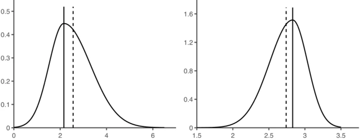
Many central banks devote a kind of stand-alone publication such as a box, a chapter, or an article to their respective definitions of risk. An example-based yet precise definition is given by the BoE in Britton, Fisher, and Whitley (1998, pp.32-33).6 According to the BoE, a risk is given by an uncertain and important event not taken into account in the central view, where the central view, i.e. the point forecast, corresponds to the mode of the forecast density. In contrast to the definition of Machina and Rothschild (2008), the probability of the event is not exogenously specified or scientifically calculable, and in contrast to the interpretation of Kilian and Manganelli (2007), the risk is unrelated to the preferences of the central bank. The balance of risks refers to the probabilities of the events mentioned producing values above or below the point forecast. The balance of risks is thus directly related to the skewness of the forecast density, which, in the case of the BoE, is measured as the difference between the mean and the mode of the forecast density. In Figure 1.1, two asymmetric forecast densities from the BoE are displayed.
The fact that the mode (and not the mean) of the forecast density serves as the BoE’s point forecast appears surprising, since aiming at the mode is associated with a rather
im-6It reads: “In deciding upon central assumptions and risks across key components of the forecast, it
may become clear that the risks are unbalanced. A good example of this is the effect of ‘windfall’ gains to consumers from the conversion of several building societies to banks in 1997. Uncertainty about the pace at which the windfalls would be spent represented a risk to the forecast of consumer spending. The Bank’s theoretical analysis suggested that only a small proportion of these gains would be spent in the first year, and correspondingly took this as a central view. In the Bank’s judgment, the risks were much greater that actual expenditure would be in excess of the central forecast assumption than that it would be less. This was an upside risk to the forecast during most of 1997. In order to produce the fan chart, only one number is needed to summarise the degree of skewness (the balance of risks). Just as with the central view and the degree of uncertainty, there is more than one possible choice of parameter. The Bank’s analysis focuses on the difference between the mean and the mode of the forecast distribution to be presented in the Report. This difference is of interest as a summary statistic of the balance of risks.”
Figure 1.1: Two of the Bank of England’s density forecasts for inflation 0 2 4 6 0 0.1 0.2 0.3 0.4 0.5 1.5 2 2.5 3 3.5 0 0.4 0.8 1.2 1.6
Note: The forecast in the left-hand panel, made in the second quarter of 2002 for the first quarter of 2004, implies an upward risk, where the mean (dashed vertical line) exceeds the mode (solid vertical line). The forecast in the right-hand panel, made in the second quarter of 1998 for the same quarter, implies a downward risk, with the mean (dashed vertical line) falling short of the mode (solid vertical line).
plausible all-or-nothing loss function of the policy maker.7 Interestingly, however, nearly all of the central banks we consider in this study as listed in Table 1.1 specifically indicate that their point forecasts are mode forecasts.8
Definitions of risk similar to the one used by the BoE can be found in the publications of other central banks. The Riksbank (1998, p.36) writes that “[...] two aspects of the forecast distribution are assessed subjectively: whether the uncertainty in the forecast differs from the historical uncertainty [...], and whether the risk of forecasting errors is symmetric, upside or downside. In the absence of information to the contrary, the risk is assumed to be symmetric. [...] A skewed uncertainty (a difference between the upside and downside risks in the assessment of a particular variable, e.g. imports) affects the distribution of the inflation forecast by the amount of the variable’s weight in the macro model. Skew is measured as the difference between the mean value and the most probable value (the mode of the distribution).” Again, the mode forecast serves as the point forecast. Further details concerning the forecasts of the Riksbank can be found in Blix and Sellin (1999). However, the Riksbank changed its forecasting procedure in 2007. Since then, it has only published symmetric forecast densities and has not mentioned the balance of risks, but just scenarios and risks. The Riksbank (2009, p.22) now states that “The forecasts in the main scenario show the path which the Riksbank expects the economy to take and is a weighted consideration of various conceivable
7
See Wallis (1999) for a discussion.
8From Table 1.1, only the Bank of Israel and the Swiss National Bank do not explicitly characterize the
meaning of their point forecasts. Moreover, the Bank of Japan and the Federal Reserve do not produce unified forecasts but instead publish summary statistics and histograms of modal forecasts from individual policy makers. The European Central Bank only publishes forecast ranges.
development paths (scenarios) and risks”; therefore, its main forecast currently seems to be a mean forecast. The Norges Bank appears to use the same approach.
Other central banks have followed the path set out by the BoE and the Riksbank. For example, the Magyar Nemzeti Bank (2004, p.108) writes that “The method that we follow in preparing fan charts broadly corresponds to that of the Bank of England, and the same holds true for the Swedish method”.
The Federal Reserve (2008, p.45) explains that the members of the Board of Governors and the presidents of the Federal Reserve Banks “provide judgements as to whether the risks to their projections are weighted to the upside, downside, or are broadly balanced. That is, participants judge whether each variable is more likely to be above or below their projections of the most likely outcome”. Hence, in contrast to the approaches mentioned so far, the risk assessments are only qualitative (naming upside, downside, or broadly balanced risks) and not quantitative. This means that there is no number attached to the risk forecasts; only the direction of the risk is given. The same applies to the risk forecasts of the European Central Bank (henceforth ECB). For example, the ECB (2010, p.6) states that “In the Governing Council’s assessment, the risks to this improved economic outlook are slightly tilted to the downside”.9
Several other central banks also link the overall forecast risks to the asymmetry of the forecast density, among them the Bank of Canada, the Banco Central de Chile, the Banco de España, the Bank of Japan, the Banco de Portugal, the Deutsche Bundesbank, and the International Monetary Fund (henceforth IMF).10 Details concerning the corresponding references are provided below.
We also found central banks which regularly report their assessments of individual risks but which do not always mention the balance of these risks. For example, the Reserve Bank of Australia (2008, p.68) states that “Risks to these forecasts can be identified in both directions. A further deterioration in the outlook for global growth would be the main source of downside risk to the forecasts for domestic activity”. Another example is the Swiss National Bank (2010a, p.40), which declares that “The biggest risk for the global economy is the continued increase in tension on financial markets [...]. At the same time, there are upside risks for the global economy [...]”. In both cases, no overall assessment of risks follows. Yet
9However, the ECB often also mentions “risks to price stability”, where the term ‘risks’ instead appears
to refer to the possibility that the ECB might not achieve its “aim of keeping inflation rates below, but close to, 2% over the medium term” (ECB, 2010, p. 6). In this case, the risks are apparently unrelated to the asymmetry of a forecast density. Note that the risks to price stability can also be asymmetric, as described in the statements: “The information that has become available [...] has confirmed that [...] upside risks to price stability over the medium term prevail” (ECB, 2008, p.5). Yet this asymmetry supposedly just refers to the probability of observing inflation rates above 2% over the medium term being larger than 50%, and is therefore also unrelated to the asymmetry of forecast densities.
10
The IMF is an intergovernmental organization, but we consider it here because its interpretation of risk forecasts is identical to that used by most central banks.
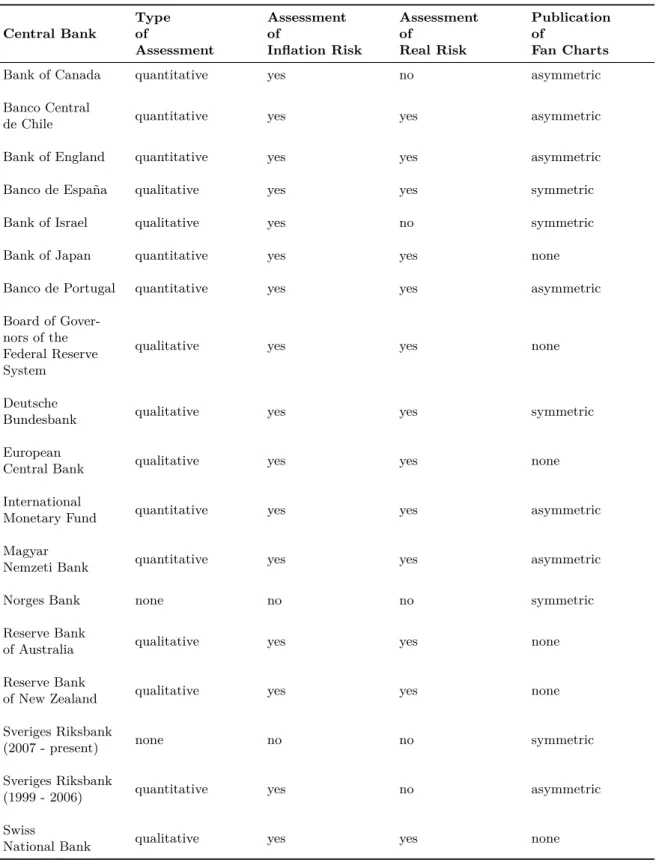
Table 1.1: Central bank assessments of macroeconomic balances of risks
Type Assessment Assessment Publication
Central Bank of of of of
Assessment Inflation Risk Real Risk Fan Charts
Bank of Canada quantitative yes no asymmetric
Banco Central
quantitative yes yes asymmetric
de Chile
Bank of England quantitative yes yes asymmetric
Banco de España qualitative yes yes symmetric
Bank of Israel qualitative yes no symmetric
Bank of Japan quantitative yes yes none
Banco de Portugal quantitative yes yes asymmetric
Board of
Gover-qualitative yes yes none
nors of the Federal Reserve System
Deutsche
qualitative yes yes symmetric
Bundesbank European
qualitative yes yes none
Central Bank International
quantitative yes yes asymmetric
Monetary Fund Magyar
quantitative yes yes asymmetric
Nemzeti Bank
Norges Bank none no no symmetric
Reserve Bank
qualitative yes yes none
of Australia Reserve Bank
qualitative yes yes none
of New Zealand Sveriges Riksbank
none no no symmetric
(2007 - present) Sveriges Riksbank
quantitative yes no asymmetric
(1999 - 2006) Swiss
qualitative yes yes none
sometimes such an assessment is made by these central banks.11 The Reserve Bank of New Zealand behaves similarly to the two aforementioned central banks, making clear statements concerning the overall risks on some occasions and mentioning only individual risks on others. The same applies to the Bank of Israel.
In Table 1.1, we present an overview of the risk forecasting practices of several central banks. Of course, this table only reflects the current situation, and the approaches to risk forecasting might change over time, as in the case of the Riksbank. Moreover, in some cases we have not been able to discover statements concerning the balance of risks, but it is not impossible that these exist.12 All central banks shown in the table regularly discuss risks to their forecasts.13 Furthermore, as mentioned above, almost all of these central banks use the mode forecast as their central forecast.
All central banks shown in the table which make precise statements concerning the meaning of the balance of risks use at least one of the following definitions. If the balance of risks for a certain variable is tilted to the upside, this means that the expected value of that variable exceeds the most likely value (i.e. the point forecast which is identical to the mode forecast), that the probability of an outturn above the point forecast is more likely than an outturn below, or that the forecast density is positively skewed.14 Thus balance-of-risks statements are supposed to contain information about the potential asymmetry of the forecast density.
It should be noted that, for many asymmetric distributions, the above-mentioned in-equalitiesE[Y]> mode(Y), P(y > mode(Y))> P(y < mode(Y)), andE[(Y −E[Y])3]>0 imply each other.15 This holds, for example, in case of the two-piece normal distribution used
by the BoE, the Magyar Nemzeti Bank, the IMF and the Riksbank (until 2006) for their asymmetric fan charts.16 Therefore, potential differences in the technical definitions of the balance of risks are probably irrelevant in actual practice.
It is perfectly possible for a central bank to consider the balance of risks to be asymmet-ric and nevertheless publish symmetasymmet-ric fan charts, as in the case of the Deutsche Bundesbank, the Banco de España, or the Bank of Israel. This could be due to the fact that these central banks, like many others, assess the balance of risks in a qualitative manner only. Asymmet-ric fan charts tend to be used if quantitative risk assessments are produced. The Banco de
11For example, the Swiss National Bank (2010b, p.26) claims that “At present, the upside and downside
risks are relatively balanced” for output growth.
12We corresponded with members of several central banks in order to minimize the possibility of certain
definitions having slipped our attention.
13
Table 1.6 in Appendix A.1 lists where these discussions can be found.
14
In Appendix A.1, we provide the references on which several of the statements made above and Table 1.1 are based.
15The same applies to the reversed inequalitiesE[Y]< mode(Y), P(y > mode(Y))< P(y < mode(Y))
andE[(Y −E[Y])3]<0. E[Y] denotes the expectation ofY andP(A) the probability of eventA.
Portugal and the Riksbank (1999-2006) are the only central banks which also release figures measuring the risk of the forecast density in their main publications.17 The Banco de Portugal
shows the probabilities of an outturn below the central projection. The Riksbank (1999-2006) publishes the values of the mode and the mean of the forecast density.
Reading through central bank publications, it seems that risks to inflation or other aggregates are commonly identified via risks to variables that determine these aggregates. For example, an upward risk to inflation might be caused by an upward risk to oil prices, to the value-added tax (henceforth VAT) rate or by a risk of the domestic currency depreciating. Thus, in order to correctly forecast the risks to inflation, one has to forecast the risks to these determinants. Actually, the process of risk forecasting could be thought of as a three-step process. In the first step, those determinants which are subject to forecast risks have to be identified. In the second step, these risks must be quantified, and in the third step, their impact on the aggregate of interest has to be calculated.
All of these steps appear extremely demanding. The first step requires the identification of variables whose most likely future paths (represented by the mode forecast) differ from their expected future paths (represented by the mean forecast). This might be possible for fiscal variables like the VAT rate, where one could imagine that a certain rate is likely, but that an alternative rate is being discussed by the government at the time the forecast is made. For variables like oil prices and exchange rates, however, this task is very challenging. The subsequent quantification of the identified risks appears fairly difficult as well. Elekdag and Kannan (2009) propose methods for accomplishing this task which can be applied to certain variables. However, their empirical performance is not evaluated. Apparently, most central banks rely on judgement for identifying as well as quantifying risks. Yet even if the risks to determinants are correctly identified and quantified, assessing their impact on the aggregate of interest is no trivial matter, as explained in Pinheiro and Esteves (2010).
To summarize, all central banks considered discuss risks to their forecasts, and many of them also assess the balance of these risks. The balance of risks is supposed to contain information about the asymmetry of the forecast density. The published point forecast corre-sponds to the mode of the forecast density for almost all central banks. In the following, the term ‘risk forecast’ will refer to the balance-of-risks forecast, i.e. to a potentially asymmetric forecast density. It will thus not denote the assessment of certain individual risks without the evaluation of their overall effect on the forecast variable of interest.
17Figures for the BoE’s and the Magyar Nemzeti Bank’s density forecasts can be downloaded from the
1.3
Data
1.3.1 Data Sources
The risk forecasting record of most central banks is very limited. As explained in Knüppel and Schultefrankenfeld (2011), inference concerning risk forecasts tends to be easier with quantitative than with qualitative risk forecasts. Therefore, we focus on data sources where quantitative risk forecasts are available. The first quantitative risk forecast that we are aware of was published by the BoE in its Inflation Report from February 1996 for inflation.18 As mentioned before, the Riksbank issued quantitative risk assessments from 1999 to 2006. Our subsequent analysis will be restricted to the risk forecasts of these two central banks, because the quantitative risk forecasts of the other institutions shown in Table 1.1 are (still) unsuitable for evaluation purposes.19
The BoE and the Riksbank use the two-piece normal distribution (henceforth tpn -distribution) as described, for example, in Wallis (2004, p.66). Our analysis utilizes the BoE’s forecasts for inflation, based on the assumption that the future official Bank Rate, i.e. the interest rate paid on commercial bank reserves, follows a path implied by market interest rates.20 In line with Elder, Kapetanios, Taylor, and Yates (2005), for the purpose of forecast evaluations we consider this assumption more adequate than that of a constant official Bank Rate. The forecast and inflation data range from the first quarter of 1998 (henceforth 1998Q1) - the first time the aforementioned interest assumption was used - to 2010Q2. Each of the BoE’s quarterly projections covers the current and the subsequent 8 quarters. For some forecasts, mean and mode forecast coincide, which results in a risk forecast equal to zero. This means that the risks to the inflation forecast are balanced.21 The BoE publishes several parameters of the forecast densities that allow a straightforward calculation of the Pearson mode skewness which will serve as our risk measure. The Pearson mode skewness of a density is defined as the mean-mode difference divided by the standard deviation.
18
According to the numerical parameters that can be downloaded athttp://www.bankofengland.co.uk/ publications/inflationreport/irprobab.htm, the skewness of the forecast density then differed from zero for the first time.
19
The Banco de Portugal started to publish quantitative risk forecasts in December 2003, but these are annual forecasts, which means that only very few observations are available. The IMF and the Bank of Japan only release annual risk forecasts, too. The Bank of Canada and the Banco de Chile do not publish data which allow a calculation of their quantitative forecast risks. Finally, the quantitative risk forecasting record of the Magyar Nemzeti Bank dates back to its Inflation Report from November 2002, and its forecasts have a quarterly frequency. However, the magnitudes of the asymmetries we backed out from its density forecast data are far too small for reliable inference about risk forecast optimality and informativeness. The asymmetries were backed out in a similar way as described for the Riksbank in Appendix A.2.2. Further details are available upon request.
20
Until 2003, the BoE used to forecast the inflation of the All Items Retail Price Index excluding mortgage interest payments (RPIX). Since 2004, it has forecast CPI inflation.
21
The BoE also publishes risk forecasts for GDP. We do not study these forecasts here, since the analysis of GDP risk forecasts would be more complicated due to the effects of data revisions. Such revisions play a substantial role for the assessment of the BoE’s GDP forecasts, as noted by Elder et al. (2005).
Our forecast data set from the Riksbank starts in December 1999, when the data used to produce the fan charts of the respective Inflation Report were made publicly available on the Riksbank’s website for the first time.22 The last asymmetric fan chart appeared in October 2006. From 1999 to 2005, there were always four Inflation Reports per year, namely in February/March/April, May/June, October, and December. Like the Riksbank, we will refer to these as the Inflation Reports y:1, y:2, y:3, and y:4, respectively, where ‘y’ stands for the year. There was no Inflation Report 2006:4, and since 2007, the fan charts of the Monetary Policy Reports, which succeeded the Inflation Reports, have always been symmetric. Therefore, our data sample covers the forecasts from the Inflation Reports from 1999:4 to 2006:3.23
A potential drawback of the data from the Riksbank is given by the constant interest rate assumption underlying the forecasts in the Inflation Reports 1999:4 to 2005:2, i.e. it was assumed that the interest rates do not change during the forecasting period, but remain on the level they had attained at the time the forecast was produced. Starting with the Inflation Report 2005:3, the forecasts have been conditioned on interest rates expected by market participants.24
In the case of a constant interest rate assumption, it might be difficult to assess the optimality of risk forecasts, at least for larger horizons. For example, if the constant interest rate assumption leads to inflation forecasts that exceed the target at the relevant policy horizon, the policy maker is likely to raise the policy rate to dampen inflation. Thus, the inflation forecast error mainly depends on the point forecast for inflation, and only to a very limited extent on the risk forecast.25 For short horizons, however, testing for risk forecast
optimality should be possible even with a constant interest rate assumption for two reasons. Firstly, a constant interest rate assumption is probably a good approximation to the behavior of interest rates in the short run. Secondly, inflation responds to changes in the interest rate only with a certain delay. Therefore, in case of the Riksbank, we will only consider risk forecasts for up to four quarters ahead.
The Riksbank forecasts two monthly inflation measures, where we decide to focus on CPI inflation only. From the available 24 forecast horizons, we use every third monthly forecast for up to four quarters ahead. We are therefore left with 5 forecast horizons, always with one observation per quarter.26 The shortest forecast horizon is chosen such that it
22
Seehttp://www.riksbank.se/templates/DocumentList.aspx?id=5031.
23Unfortunately, the forecast data from the Inflation Report 2000:1 are not available, which means that our
sample contains only 27 instead of 28 forecasts.
24See Sveriges Riksbank (2005, p.57). 25
Only if the central inflation forecast implies that inflation will be close to target, could the inflation forecast error be well predicted by the risk forecast if the risk forecast is optimal.
26
Using all monthly forecasts yields practically no additional insights, since the monthly risk forecasts are quantitatively very similar for adjacent forecast horizons, and the forecast errors of adjacent horizons are often similar, too. Moreover, the results can be compared more easily to those for the BoE using every third monthly
Figure 1.2: Scatter plots for the Bank of England and the Sveriges Riksbank BoE,h= 0 −0.5 0 0.5 −4 0 4 BoE,h= 2 −0.5 0 0.5 −4 0 4 BoE,h= 4 −0.5 0 0.5 −4 0 4 BoE,h= 6 −0.5 0 0.5 −4 0 4 BoE,h= 8 −0.5 0 0.5 −4 0 4 Riksbank,h= 0 −0.5 0 0.5 −4 0 4 Riksbank,h= 2 −0.5 0 0.5 −4 0 4 Riksbank,h= 4 −0.5 0 0.5 −4 0 4 All −0.5 0 0.5 −4 0 4
Note: The forecast Pearson mode skewness is shown on theX-axis, the scaled forecast error of the mode on theY-axis. The lower right-hand panel is a scatter plot of all data of the Bank of England forh= 0,2,4,6,8 and of the Sveriges Riksbank forh= 0,2,4.
contains a forecast for the month of the publication of the Inflation Report, meaning that this forecast is actually a nowcast. Thus, we consider the Riksbank’s 0-, 3-, 6-, 9-, and 12-month-ahead forecasts. In contrast to the BoE, the Riksbank only published the mode of the forecast density and the values of several quantiles. From these data and the corresponding statements in the Inflation Reports, we carefully back out the parameters which permit calculation of the Pearson mode skewness of the forecast densities. Details are provided in Appendix A.2.2. forecast only.
Table 1.2: Summary statistics for forecast data of the Bank of England and the Sveriges Riksbank h 0 2 4 6 8 Bank of England Sample average ˆ mt+h|t 2.35 2.23 2.06 2.03 2.14 ˆ µt+h|t−mˆt+h|t 0.01 0.03 0.03 0.04 0.04 ˆ σ2 t+h|t 0.08 0.29 0.43 0.58 0.77 Interquartile range ˆ mt+h|t 0.71 0.48 0.58 0.52 0.47 ˆ µt+h|t−mˆt+h|t 0.03 0.07 0.09 0.11 0.20 ˆ σ2t+h|t 0.05 0.14 0.16 0.24 0.42 Sveriges Riksbank Sample average ˆ mt+h|t 1.44 1.46 1.71 ˆ µt+h|t−mˆt+h|t 0.00 0.01 0.02 ˆ σ2 t+h|t 0.09 0.24 0.54 Interquartile range ˆ mt+h|t 1.52 0.85 0.67 ˆ µt+h|t−mˆt+h|t 0.00 0.03 0.09 ˆ σ2 t+h|t 0.01 0.02 0.05
Note: The sample size equalsT = 50 for the Bank of England andT = 27 for the Sveriges Riksbank.
The risk forecasts of the BoE and the Riksbank as measured by the Pearson mode skewness of the forecast densities are displayed in Tables 1.7 and 1.8 in Appendix A.2 for all forecast horizons. For ease of exposition, in the following we focus on the results for even horizons, i.e. BoE results forh= 0,2,4,6,8 and Riksbank results for h= 0,2,4.27 No major
insights are lost by leaving the odd horizons aside.
1.3.2 Summary Statistics
Before turning to the empirical tests, it is useful to take a brief look at the forecast risks and the associated realized risks used in this study. The forecast risk, measured by the Pearson mode skewness, is defined as (ˆµt+h|t−mˆt+h|t)/σˆt+h|t, where ˆµt+h|t is the mean forecast for period t+h made in period t, ˆmt+h|t is the corresponding mode forecast, and ˆσt+h|t is the corresponding forecast of the standard deviation.28 Our measure of realized risk is given by the scaled mode forecast error, i.e. by (yt+h−mˆt+h|t)/σˆt+h|t, whereyt+h is the realization of
27
These quarterly horizons correspond to the the Riksbank’s 0-, 6-, and 12-month-ahead forecasts, respec-tively.
28
Further explanations concerning the use of the Pearson mode skewness follow in Section 1.4 and compu-tational details are provided in Appendix A.2.1.
Figure 1.3: Plots of the differences between the mean forecast and the mode forecast for the Bank of England and the Sveriges Riksbank
BoE,h= 0 1998Q1 2002Q1 2006Q1 2010Q1 0 0.2 0.4 BoE,h= 2 1998Q1 2002Q1 2006Q1 2010Q1 0 0.2 0.4 BoE,h= 4 1998Q1 2002Q1 2006Q1 2010Q1 −0.2 0 0.2 0.4 BoE,h= 6 1998Q1 2002Q1 2006Q1 2010Q1 0 0.2 0.4 BoE,h= 8 1998Q1 2002Q1 2006Q1 2010Q1 −0.2 0 0.2 0.4 Riksbank,h= 0 1999Q4 2001Q4 2003Q4 2005Q4 0 0.1 0.2 Riksbank,h= 2 1999Q4 2001Q4 2003Q4 2005Q4 0 0.1 0.2 Riksbank,h= 4 1999Q4 2001Q4 2003Q4 2005Q4 −0.1 0 0.1 0.2
the forecast variable in periodt+h. Figure 1.2 shows horizon-specific scatter plots of forecast and realized risks for the BoE and the Riksbank. The lower right-hand panel contains all data from the previous plots summarized in a single scatter plot. The largest forecast risks equal about 0.5, the smallest about −0.3. The realized risks, i.e. the scaled mode forecast errors, range from about −2.6 to about 4.5. For a large number of periods, the risks were actually forecast to be balanced.
If the risk forecasts are optimal, most points in the scatter plots should be located in the first and third quadrant. If the risk forecasts are not informative, the points should spread broadly evenly above and below the zero-line.29 Thus, the regression lines in all BoE data plots in Figure 1.2 rather suggest a lack of information content, because they are not
upward-sloping. In contrast, the regression lines for h = 2 and h = 4 for the Riksbank are upward-sloping, but the scatter plots indicate that there is considerable uncertainty about these slopes. Finally, the line computed for the entire sample of risk forecasts is slightly downward-sloping.
In Table 1.3.2, we provide summary statistics for the forecast data of the BoE and the Riksbank. While the sample averages of the difference between mean and mode forecasts increase with the forecast horizon, they remain very close to zero. The sample averages of the forecast variance grow substantially with the horizon, indicating the increasing forecast uncertainty. While the interquartile ranges for the forecasts of mean-mode differences and variances also increase with the forecast horizon, for the mode forecasts they do not. The latter finding is, of course, due to the fact that the long-run inflation point forecasts tend to be close to the inflation target.
Figure 1.3 shows the differences between mean and mode forecasts. It reveals that serial correlation in these differences seems to be fairly contained. In contrast, there are pronounced correlations across horizons.30
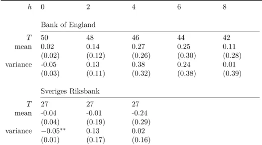
1.3.3 Bias Tests
As explained in Knüppel and Schultefrankenfeld (2011), when applying the framework of regression-based tests for forecast optimality as proposed by Mincer and Zarnowitz (1969) to risk forecasts, estimates of the intercept and the slope coefficient might be biased since the forecast data used to construct the Pearson mode skewness might themselves be biased.
Testing for a bias of the mean forecasts is interesting in itself. In addition, if the mean forecast ˆµt+h|t is biased, the squared forecast error of the mean,
yt+h−µˆt+h|t
2
, is unlikely to be a good measure for the variance of inflation realizationyt+h. Therefore, it is useful to test whether an estimate of the interceptcin the equation
yt+h−µˆt+h|t=c+εt+h (1.1)
is equal to zero. If the true variances, and hence the true standard deviations σt+h are, on average, smaller than ˆσt+h|t, estimates of intercept and slope in a Mincer-Zarnowitz-type regression for risk forecasts are biased towards zero.31 Conversely, ifσ
t+h is larger than ˆσt+h|t, the estimates of intercept and slope are biased away from zero. Thus, it is important to test for unbiasedness of the volatility forecasts, too. Analogously to above, in the equation
yt+h−µˆt+h|t
2
−σˆt2+h|t=c+εt+h, (1.2)
30This can also be seen in Tables 1.7 and 1.8. 31