Faculty of Engineering and Information
Sciences - Papers: Part A Faculty of Engineering and Information Sciences 1-1-2014
An approximation method for improving dynamic network model fitting
An approximation method for improving dynamic network model fitting
Nicole B. CarnegieHarvard School of Public Health
Pavel N. Krivitsky
University of Wollongong, [email protected]
David R. Hunter
Pennsylvania State University
Steven M. Goodreau
University of Washington
Follow this and additional works at: https://ro.uow.edu.au/eispapers
Part of the Engineering Commons, and the Science and Technology Studies Commons
Recommended Citation Recommended Citation
Carnegie, Nicole B.; Krivitsky, Pavel N.; Hunter, David R.; and Goodreau, Steven M., "An approximation method for improving dynamic network model fitting" (2014). Faculty of Engineering and Information Sciences - Papers: Part A. 3237.
networks that change over time. One promising model is the separable temporal exponential-family random graph model (ERGM) of Krivitsky and Handcock, which treats the formation and dissolution of ties in parallel at each time step as independent ERGMs. However, the computational cost of fitting these models can be substantial, particularly for large, sparse networks. Fitting cross-sectional models for observations of a network at a single point in time, while still a non-negligible computational burden, is much easier. This paper examines model fitting when the available data consist of independent measures of cross-sectional network structure and the duration of relationships under the assumption of
stationarity. We introduce a simple approximation to the dynamic parameters for sparse networks with relationships of moderate or long duration and show that the approximation method works best in precisely those cases where parameter estimation is most likely to fail—networks with very little change at each time step. We consider a variety of cases: Bernoulli formation and dissolution of ties,
independent-tie formation and Bernoulli dissolution, independent-tie formation and dissolution, and dependent-tie formation models.
Keywords Keywords
Separable temporal exponential random graph models (STERGMs), model fitting, exponential random graph models (ERGMs), Markov chain Monte Carlo
Disciplines Disciplines
Engineering | Science and Technology Studies
Publication Details Publication Details
Carnegie, N. Bohme., Krivitsky, P. N., Hunter, D. R. & Goodreau, S. M. (2015). An approximation method for improving dynamic network model fitting. Journal of Computational and Graphical Statistics, 24 (2), 502-519.
An approximation method for improving dynamic
network model fitting
Nicole Bohme Carnegie
1, Pavel N. Krivitsky
2, David R. Hunter
3, and Steven
M. Goodreau
41
Harvard School of Public Health
2University of Wollongong
3Pennsylvania State University
4
University of Washington
Abstract
There has been a great deal of interest recently in the modeling and simulation of dynamic networks, i.e., networks that change over time. One promising model is the separable temporal exponential-family random graph model (ERGM) of Krivitsky and Handcock, which treats the formation and dissolution of ties in parallel at each time step as independent ERGMs. However, the computational cost of fitting these models can be substantial, particularly for large, sparse networks. Fitting cross-sectional models for observations of a network at a single point in time, while still a non-negligible computational burden, is much easier. This paper examines model fitting when the available data consist of independent measures of cross-sectional network struc-ture and the duration of relationships under the assumption of stationarity. We introduce a simple approximation to the dynamic parameters for sparse networks with relationships of moderate or long duration and show that the approximation method works best in precisely those cases where parameter estimation is most likely to fail—networks with very little change at each time step. We consider a variety of cases: Bernoulli formation and dissolution of ties, independent-tie for-mation and Bernoulli dissolution, independent-tie forfor-mation and dissolution, and dependent-tie formation models.
Key Words: Separable temporal exponential random graph models (STERGMs), model fitting,
1
Introduction
Dynamic social networks—those in which relations form and break over time—have long been an area of research interest, to understand both the nature of the dynamics themselves (Holland and Leinhardt, 1977; Runger and Wasserman, 1980; Wasserman, 1980; Frank, 1991; Doreian and Stokman, 1997) and their implications for processes like the flow of information or disease (Morris and Kretzschmar, 2000; Mercken et al., 2009; Sasovova et al., 2010; Jack et al., 2010; Weerman, 2011). This field remains active, with a variety of models for dynamic networks being explored (Aral et al., 2009; Snijders, 2001; Snijders et al., 2007; Snijders and Koskinen, 2013).
Recently, the exponential-family random graph modeling (ERGM) framework has become a popular approach for conducting inference on network structure, due to its generalizability and its basis in exponential family theory, a common and parsimonious statistical approach (Frank and Strauss, 1986; Strauss and Ikeda, 1990; Wasserman and Pattison, 1996; Robins and Pattison, 2001; Snijders et al., 2006; Robins and Morris, 2007; Hunter et al., 2008a, for example). For many years, the application of the ERGM framework was limited to static, or cross-sectional, network datasets. However, recent developments have extended ERGMs to the modeling of dynamic networks, in-cluding the separable temporal ERGM (STERGM) approach of Krivitsky and Handcock (2012), among others (Snijders and Koskinen, 2013). The STERGM is a form of discrete temporal ERGM of Hanneke et al. (2010) that independently models the formation and dissolution of ties over time. This allows for independent control of the incidence of tie formation and of relational duration. This article considers applications of the STERGM where the available data consist of measures of both the cross-sectional network structure and the duration of relationships. These data are used to model the dynamic evolution of the network under the assumption that they come from a stochastic process that has reached equilibrium. In this paper, we concentrate on examples in which the set of actors and their attributes remains fixed while their pairwise relationships can stochastically form and dissolve. The approach described in this paper can be easily extended to simulating networks with changing sets of actors, using the approach of Krivitsky et al. (2011).
dy-available about networks of interest, with sexual partnership networks being a major example. Krivitsky (2012a) fits STERGMs to cross-sectional and egocentric network data using gradient descent to find the generalized methods of moments estimator (GMME) for the parameters, an approach that has been used in multiple applications (e.g., Morris et al., 2009; Goodreau et al., 2010). In each of these cases, parameters for the relational dissolution process were assumed, and starting values for the estimation of the formation model were obtained from fitting a traditional static ERGM on the cross-sectional data. Although this approach produces stable parameter es-timates for these specific cases, in general it suffers from two crucial limitations. First, it can be very time-consuming and memory-intensive, especially for networks that are large and sparse and have long relational durations. For example, fitting a STERGM in this way on a network of 10,000 nodes with a relational duration of about 1100 time steps and a mean degree of 0.4 takes several days on a high-performance UNIX cluster and is not amenable to parallelization. Moreover, as is often the case with ERGMs more generally, the model fitting process can be unstable if the start-ing values are far from the true parameters, and may fail to converge even when the model is good (Hummel et al., 2012).
In this paper, we give technical justification for a novel approximation method using parameter estimates from a static ERGM and estimates of the duration of relationships to generate starting values for the existing algorithm. In practice, we have found that this simple adjustment results in substantially better performance than fitting a STERGM using the traditional approach. Not only does the algorithm generally converge much faster to reasonable parameter estimates when started from the new values, but in many cases the adjusted starting values themselves are an ade-quate estimate of the STERGM parameters, and it is unnecessary to run the fitting algorithm. The approach requires the same information used for the existing approach—a single cross-sectional network or target cross-sectional statistics plus mean relational duration—and is found to work best in precisely those cases when STERGM estimation is slowest and most unstable.
The approximation procedure described in this paper was motivated by challenges encountered in two large network simulation projects. Both projects attempt to model the potential effect of in-terventions to prevent the spread of HIV over sexual networks. We use one of these projects, which
models the HIV epidemic among men who have sex with men (MSM) in North and South Amer-ica and the potential effect of a variety of prevention interventions on those epidemics (Goodreau et al., 2012) as a motivating example in this paper (see Sections 4.2 and 5.1).
In Section 2, we give a short description of the separable temporal exponential random graph model and the estimation thereof using cross-sectional or egocentric network data and independent data on relational duration. In Section 3, we show that a simple correction to the static ERGM parameters performs well as an approximation to STERGM parameters in the Bernoulli model case. In Section 4, we extend this to relational independence models for formation and dissolution, with an application to modeling the spread of HIV among men who have sex with men in the dyadic independence case. Section 5 discusses the utility of the approximation in the relational dependence case through simulations and an extension of the application.
2
Brief description of the STERGM
We first review the ERGM framework for cross-sectional or static networks, observed at a single point in time. Following the notation of Krivitsky and Handcock (2012), letY⊆ {1, . . . ,n}2be the
set of potential ties among n nodes, ordered for directed networks and unordered for undirected. We can represent a network y as a set of ties, with the set of possible sets of ties,Y ⊆ 2Y, being the sample space: y∈ Y. Let yi j be 1 if (i, j) ∈y—a relation of interest exists from i to j—and 0
otherwise.
The network also has an associated covariate array X containing attributes of the nodes, the potential ties, or both. An exponential-family random graph model (ERGM) represents the pmf of
Y as a function of a p-vector of network statistics g(Y,X), with parametersθ∈Rp, as follows:
Prθ(Y=y|X)=
exp{θ∙g(y,X)}
k(θ,X,Y) , (2.1)
where the normalizing constant k(θ,X,Y)=Py0∈Yexp{θ∙g(y0,X)}is a summation over the space of possible networks on n nodes, Y. Where Y and X are held constant, as in a typical cross-sectional model, they may be suppressed in the notation. Here, on the other hand, the dependence
In modeling the transition from a network Yt−1 at time t − 1 to a network Yt at time t, the
separable temporal ERGM assumes the formation and dissolution of ties to occur independently from each other within each time step, with each half of the process modeled as an ERGM. For two networks (sets of ties) y,y0 ∈ Y, let y ⊇ y0if any tie present in y0 is also present in y. Define
Y+(y) = {y0 ∈ Y : y0 ⊇ y}, the set of networks that can be constructed by forming ties in y; and
Y−(y)={y0 ∈ Y: y0 ⊆y}, the set of networks that can be constructed by dissolving ties in y. Given yt−1, a formation network Y+ is generated from an ERGM controlled by a p-vector of
formation parametersθ+and formation statistics g+(y+,X), conditional on only adding ties:
PrY+ =y+|Yt−1;θ+ = exp{θ+∙g+(y+,X)}
k θ+,X,Y+(Yt−1), y
+ ∈ Y+(yt−1). (2.2)
A dissolution network Y−is simultaneously generated from an ERGM controlled by a (possibly different) q-vector of dissolution parametersθ−and corresponding statistics g−(y−,X), conditional
on only dissolving ties from yt−1:
PrY− =y−|Yt−1;θ− = exp{θ
−∙g−(y−,X)}
k θ−,X,Y−(Yt−1), y
− ∈ Y−(yt−1). (2.3)
The cross-sectional network at time t is then constructed by applying the changes in Y+and Y−to
yt−1: Yt =Yt−1∪(Y+\Yt−1)\(Yt−1\Y−).
This transition process is ergodic: a series of networks generated from this process converges to an equilibrium distribution of networks Pr Yt =y;θ+, θ−. To the extent that the observed net-work y is a consequence of the long-run evolution of the social process being modeled, it may be modeled as a draw from this equilibrium distribution.
The realism of the assumption of separability depends to a certain extent on the definition of a time step. If moving from t−1 to t represents a year’s worth of network evolution, this assumption will be less plausible than if it represents a daily change.
Note that the underlying, network-to-network transition process does not change over time, but rather the set of existing relationships evolves in a manner consistent with the stochastic process as specified byθ+,θ−, and the particular statistics that make up g+(y+,X) and g−(y−,X).
Implicit in this model is a Markovian assumption that the survival of a relationship from time t to t+1 is, conditional on its existence at t, independent of what happened before t. Also implicit
under a relational independence dissolution model is a geometric distribution for the relational duration for each tie, with mean given by the reciprocal of the probability of survival for that tie. The probability of survival may vary across dyads; however, under a strict Bernoulli dissolution model, in which all ties have an equal probability (1−p) of survival, relational durations will follow
a geometric distribution with mean duration d and probability of dissolution per time step p=1/d.
This process can be captured by including a single statistic for the edge count in g−(y−,X); its
parameter θ− should equal the log-odds of a relation surviving the time step (Krivitsky, 2012b), i.e.,θ−= log[(1−p)/p]= log(d−1).
We assume from now on that the average duration(s) are specified and thus that θ− is known. This would be an appropriate assumption, for instance, if we wished to simulate a dynamic network from a cross-sectional observation of a network together with information on the duration of ties, as with Morris et al. (2009). In our examples, we takeθ−to be a scalar, implying a single distribution of durations for the whole population, but the theory developed supports extension to any relational independence model for dissolution.
Recall that we are fitting a dynamic model only to information about a single cross-sectional network, with some tie duration information. In that setting, to the extent that an assumption can be made that the observed network is a draw from the stationary distribution of the STERGM process (which is ergodic), parameter valuesθ+may be estimated using the generalized
method-of-moments approach. The generalized method-of-method-of-moments estimator (GMME) in the static ERGM is the solution to the equation Eθ{g(Y,X)} = g(y,X), where y is the observed network and
Eθ{g(Y,X)} is the expected value of the network statistics of interest under the stationary
dis-tribution induced byθ.
Parameter estimation is accomplished using the procedure for obtaining the GMME described in Krivitsky (2012a), with a modification to the selection of starting values. Initial parameter estimates θ+
0 are either directly specified or generated from simple estimation methods, such as
estimating parameters in a cross-sectional model for dyadic independence terms and setting de-pendence terms to 0.
Eθ(g(Y,X)) by simulation. If the network evolves slowly, successive networks drawn from the
model are likely to be highly autocorrelated. Thus, to obtain a sufficiently precise estimate of
Eθ(g(Y,X)) we must simulate a very long series of such networks—a time-consuming process.
As is common in ERG modeling, if the starting values θ+
0 are far from the GMME, the
distri-bution of sampled networks is likely to be degenerate, making it next to impossible to estimate the necessary moments. Consequently, the algorithm fails to converge in a feasible timeframe. Thus, we require a value for θ+
0 that produces networks that are reasonably similar to the target. We
introduce one such starting point below in Section 3.
Throughout this paper, we use the statnet suite of packages (Handcock et al., 2008) in R (R Development Core Team, 2011) for simulation and model fitting.
3
Bernoulli models
We first consider the simplest case, a STERGM with a Bernoulli model for both formation and dissolution of edges. In this case, each process is controlled by a single parameter, giving an equal probability of formation (or dissolution) for all non-edges (or extant edges). We can derive the value and corresponding GMME, ˆθ+, of the formation parameterθ+as a function of edge duration
and edge density, where we define the latter to be the ratio of the number of existing edges to the total number M of possible edges. We wish to justify the following approximation to ˆθ+ for a
particular fixedθ−: ˜ θ+ def = log d 1−d ! −θ−= logit (d)−θ− ≈θˆ+, (3.1)
where d is the target edge density we want to achieve at equilibrium.
Since parameters in the STERGM control either formation or dissolution independently, we can interpret logit−1(θ+) = eθ+
(1+eθ+)−1 as the expected fraction of null edges that will become ties,
while logit−1(θ−) is the expected fraction of existing edges that will survive the time step. Let m(t) be the (random) edge density of the network at time t. At equilibrium, the average numbers of ties
created and destroyed are the same, so
E[(1−logit−1(θ−))∙m(t)∙ M]= E[logit−1(θ+)∙(1−m(t))∙ M].
Hence, if we letμ= E[m(t)], where we assume thatμdoes not depend on t because the network is at equilibrium, logit−1(θ+) 1−logit−1(θ−) = E[m(t)] 1−E[m(t)] = μ 1−μ. (3.2)
Thus, the formation parameter we wish to estimate and its corresponding GMME are
θ+ =−log 1+e θ− μ 1−μ −1 and θˆ+ =−log 1+eθ− d 1−d −1 , (3.3)
respectively, where d is the target edge density. Recall from Section 2 that the dissolution parameter
θ−, a simple transformation of the average edge duration, is assumed known.
3.1
Derivation of the approximation
To verify Approximation (3.1), we first argue that as the number of nodes n increases, the density
m(t) at equilibrium should converge to zero in probability. This assumption is justified by the fact
that for most social phenomena, mean degree is likely to stay roughly constant even as the network grows (Krivitsky et al., 2011). For example, people living in a town of 10,000 should have roughly the same numbers of relationships per person as those in a city of 10 million, and not three orders of magnitude fewer. We may express this assumption probabilistically by postulating that for a fixed time t after equilibrium is achieved, the (random) mean degree remains bounded in probability as
n→ ∞. Since mean degree=(n−1)m(t), this implies that m(t) →P 0 as n→ ∞.
The verification of Approximation (3.1) also requires the assumption that θ− → ∞. Since θ−
determines average duration of relationships in terms of a number of steps in the evolution of the network, we can make this more plausible in practice, when dealing with a network of fixed size, by changing the time scale so that this average is long (e.g., equate a single step to a day instead of a month).
Combining Equations (3.1) and (3.3) gives ˜ θ+−θˆ+= log 1+e−θ− " 1−2m 1−m #! , (3.4)
where we suppress the fixed equilibrium time t to simplify notation. The right hand side of Equa-tion (3.4) clearly tends to zero asθ−→ ∞as long as m stays bounded away from 1, so the fact that
m→P 0 yields the following result:
Proposition 1. For a Bernoulli formation and Bernoulli dissolution model, if mean degree is
as-sumed bounded in probability thenθ˜+−θˆ+ →P 0 as n→ ∞andθ−→ ∞.
3.2
Accuracy of approximation
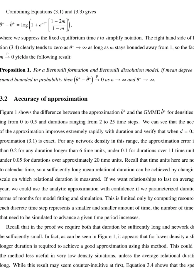
Figure 1 shows the difference between the approximation ˜θ+and the GMME ˆθ+for densities
rang-ing from 0 to 0.5 and durations rangrang-ing from 2 to 25 time steps. We can see that the accuracy of the approximation improves extremely rapidly with duration and verify that when d = 0.5, ap-proximation (3.1) is exact. For any network density in this range, the apap-proximation error is less than 0.2 for any duration longer than 6 time units, under 0.1 for durations over 11 time units and under 0.05 for durations over approximately 20 time units. Recall that time units here are not tied to calendar time, so a sufficiently long mean relational duration can be achieved by changing the scale on which relational duration is measured. If we want relationships to last on average one year, we could use the analytic approximation with confidence if we parameterized durations in terms of months for model fitting and simulation. This is limited only by computing resources: as each discrete time step represents a smaller and smaller amount of time, the number of time steps that need to be simulated to advance a given time period increases.
Recall that in the proof we require both that duration be sufficently long and network density be sufficiently small. In fact, as can be seen in Figure 1, it appears that for lower density a slightly longer duration is required to achieve a good approximation using this method. This could make the method less useful in very low-density situations, unless the average relational duration is long. While this result may seem counter-intuitive at first, Equation 3.4 shows that the speed of the approximation depends on the observed density; for m(t) close to 0.5, the speed is faster than
for m(t) close to either 0 or 1. Thus for very low or very high density, a longer average duration is needed to achieve a given margin of error in the approximation. In contrast, the expected density (arguably a more important metric than the parameter value itself) is well approximated for any duration for either density close to 0.5 or very low density; it is only in the midrange where a sufficiently long duration must be reached to obtain reasonable expected density.
4
Relational independence models
In this section, we extend the above results to models with relational independence terms in the formation and dissolution models. In a cross-sectional ERGM, relational independence means that the states of all dyads are stochastically independent (Hunter et al., 2008b), but we do not assume independence across time steps. In the case of undirected ties, relational independence is equivalent to dyadic independence.
4.1
Derivation of the approximation
We now consider STERGMs with relational independence models for formation and dissolution. Under relational independence, the vectors of network statistics are
g+(y+,X)= X (i,j)∈Y y+i jWi j+ and g−(y−,X)= X (i,j)∈Y y−i jWi j−, (4.1) where W+ i j ≡ W +
i j(X) and Wi j− ≡ Wi j−(X) are arbitrary vectors of attributes for the potential tie (i, j)
of length p and q, respectively, and y+i j (y−i j) is the indicator that this tie is contained in y+ (y−). It is common that the Wi j∗ may be written as some function of nodal covariates defined for i and
j. For instance, the Euclidean distance between nodes i and j may be expressed as a function of
their location vectors. In general, however, Wi j∗ may include entries that cannot be expressed in this way (e.g., some non-Euclidean “distances” such as shortest road distance or average driving time between locations i and j).
We make the additional assumptions that q ≤ p and the first q elements of Wi j+ are simply Wi j− for all i and j. This assumption may be justified theoretically because in many processes we are
interested in modeling, the formation of relationships is more complicated than their dissolution. For example, the creation of spousal relationships through marriage is a complex matching prob-lem, but their dissolution is simplified because there is only one possible tie to dissolve. In the examples used in this paper, the distribution of relationship lengths can be reasonably modeled by a simple geometric distribution—i.e., a Bernoulli dissolution model. Krivitsky and Handcock (2012) discuss this issue further.
Exploiting our assumption that W+
i j ⊇ Wi j−, we may generalize the approach of Equation (3.1)
by following these steps:
1. Calculate the maximum likelihood estimator, say ˆθ, for a cross-sectional ERGM for the ob-served network using sufficient statistics W+
i j; 2. Define ˜ θ+ =θˆ− θ − 0p−q . (4.2)
In other words, subtract theθ−vector from ˆθ, where the former must first be padded with p−q
zeros so that the dimensions agree. We shall take ˜θ+to be the approximation to the GMME
ˆ
θ+.
The situation of Section 3 is a special case, since in that instance we have p = q= 1 and Wi j = 1
for all (i, j). This means that the ˆθestimate may be found in closed form, namely, ˆθ = logit(d) as in Equation (3.1).
We may justify the procedure above by the following heuristic argument, which may be made rigorous by a proof analogous to that of Section 3.1. First, notice that each Yi j may be viewed as
an independent two-state Markov chain with transition probability matrix
Mi j = 11−−pqi ji j qpi ji j ,
where pi j = logit−1(Wi j−∙θ−) and qi j = logit−1(Wi j+∙θ+). Letting Oi j denote the odds of Yi j = 1 at
equilibrium, the equilibrium distribution for Yi j may be easily shown to satisfy
Oi j =
logit−1(Wi j+∙θ+)
For instance, in the case where the Yi j are identically distributed, as in Section 3, the odds are
merelyμ/(1−μ) and so Equation (4.3) reduces to Equation (3.2). The idea is that we may esti-mate Oi j via logistic regression if we assume that we observe a network at equilibrium. This is
accomplished by step 1 above; after fitting the cross-sectional ERGM, our estimate ˆOi j is simply
exp{W+
i jθ+}. Substituting ˆOi jfor Oi jand solving for Wi j+∙θ+then yields
Wi j+∙θ+
=Wi j+∙θˆ−log1−Oˆi j+exp{Wi j−∙θ−}
. (4.4)
When Wi j−∙θ− 0, the term 1 −Oˆi j on the right hand side of Equation (4.4) is negligible—we
assume by sparsity that Oi j will typically be small—and so we obtain
Wi j+∙θ+ ≈W+
i j ∙θˆ−Wi j−∙θ−.
This approximation must hold for each (i, j); furthermore, since we assumed that W+
i j ⊇ Wi j−, we
are led to the approximation of Equation (4.2). Our earlier assumption thatθ− → ∞in the case
Wi j− = 1 must now be replaced by the assumption that Wi j−∙θ− → ∞, which is how we can justify the approximation resulting from Wi j−∙θ− 0.
We find that in practice, this general method works well for arbitrary W+
i j; we explore an
appli-cation in Section 4.2. A further open question, which we explore in Section 5, is whether a similar technique applies even when the assumption of relational independence is violated.
4.2
Application: Modeling HIV spread among MSM in the US
To demonstrate the use of this approximation method in practice, we present an example from the PUMA (Prevention Umbrella for MSM in the Americas) project, which examines the potential impact of a variety of behavioral and biomedical interventions for men who have sex men (MSM) in the United States, Peru and Brazil. Our example stems from the baseline US model, which aims to model transmission prior to the roll-out of additional interventions (Goodreau et al., 2012). In the US and many other nations, HIV remains concentrated among MSM, with well over half of all new HIV diagnoses within this community (Hall et al., 2008). Rates of HIV incidence are on the rise among young MSM, and especially among young Black and Latino MSM (Prejean
et al., 2011). For this reason, the model considers sexual network data disaggregated into three race/ethnicity categories: Blacks, Latinos, and all others.
As part of developing simulation models of HIV transmission among MSM, we use a separable temporal ERGM to model main partnerships. These are defined in our study as any relationship in which men feel a close emotional connection, regardless of the type of relationship (e.g. casual dating, long-term committed partnership). Given this, the observed distribution of relationship duration is strongly right-tailed with a mode near 0. For convenience, we model this with the exponential distribution, indicated by using a constant θ− as the sole parameter in the dissolu-tion model. Casual contacts are modeled using a cross-secdissolu-tional ERGM not discussed here. To demonstrate the performance of the approximation for relational independence models, we begin by specifying the partnership formation part of the ERGM with an edge count term to control den-sity, an individual attribute of race to allow for differential rates of partnership formation across races, and partnership-level matching on race, age and preferred sexual role (strictly insertive, strictly receptive, or versatile). The formation model is thus
PrY+= y+|Yt−1;θ+∝ exp θ+(e)∙e+ X r θ+(u r)∙ur+ X r θ+(m r)∙mr +θ+(a)X k<l |(page(k)− page(l))|+X c=r,i θ+(m c)∙mc ,
where yi j = the pair of persons i and j, and yi j = 1 indicates they are partners; Yci j = the rest of
the pairs in the network, excluding the yi jpair; e=total number of partnerships of all types in the
network; ur = the number of partnerships of persons of race r; mr = the number of partnerships
with both partners of race r; mc = the number of partnerships with both partners of role class c
(which can take values i=strictly insertive or r=strictly receptive); k and l represent the actors in each main partnership. The parameters for matching on sexual role are fixed at negative infinity to enforce a prohibition on sexual encounters between either two strictly insertive men or two strictly receptive men.
deter-main partnerships. This, together with the fact that the model is stepped forward day by day, yields a dissolution parameterθ−= log(3.1∙365−1)=7.0.
Estimating the formation parameters for this model on a network of 10,000 nodes using the traditional approach outlined in Section 1 is extremely computationally intensive—on the order of days to weeks. We use instead the adjustment to the static ERGM fit discussed above as parameter estimates. We simulate a network forward in time using the parameters generated and compare the distribution of simulated network statistics to the target values taken from the observed network.
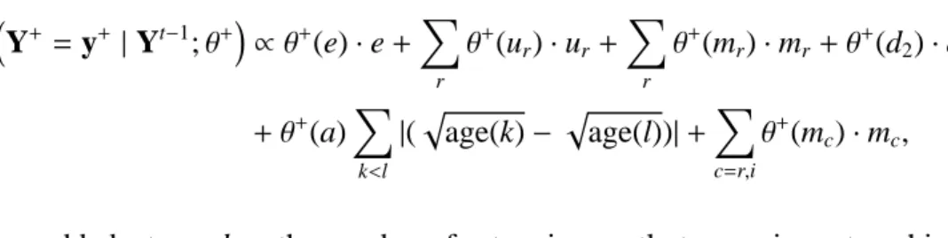
Figure 2 shows the standardized deviations of the simulated cross-sectional network statistics from their target values over the evolution of the network for 10,000 time steps. Counts of the total number of partnerships of nodes of a certain type are referred to as “node factor” terms, while counts of edges with both nodes of the same type are referred to as “node match” terms. Note that the node match terms for role class are excluded from the plot since they are coerced to be zero at all times. Since the simulation follows all steps of the MCMC chain without thinning, we expect to see some autocorrelation and “walks” away from the target over time; however, the observed statistics at each cross-section are largely within two standard deviations of the target. This indicates that the approximation has yielded reasonable estimates of the model parameters.
We expect, given the long duration and the analytic results above, that the approximate param-eter estimates would be adequate in this case, where the models for formation and dissolution are both relational independence models.
5
Relational dependence formation models
In this section, we extend our exploration of the approximation to a case with a dyadic dependent formation model. This case is generally more socially realistic than those we have investigated thus far, but analytical solutions to estimation are far less tractable. As Krivitsky (2012a) dis-cusses, any dyadic dependence, whether within a time step (where Yt
i j⊥⊥Y
t
i0j0|Y
t−1 = yt−1 for
(i, j) ,(i0, j0)), such as that fit by Krivitsky, or between time steps (where Yti j ⊥⊥Yti0j0|Yt−1 = yt−1
but Yt i j⊥⊥Y t−1 i0j0 |Y t−1 i j = y t−1
evo-lution of the network from being represented as in Section 4.1, with each potential tie evolving independently as a two-state Markov chain. Instead, in some cases it appears that this station-ary distribution is even less tractable than that of an intractable normalizing constant, a point ad-dressed by Hunter and Handcock (2006). Snijders (2001, Prop. 1) discusses a related result for continuous-time Markov models for network evolution: If the model is constrained to treat forma-tion and dissoluforma-tion symmetrically—that is, g+≡ g−andθ+ ≡θ−—then the stationary distribution is an ERGM, though this view of the model is less interpretable than the STERGM (Krivitsky and Handcock, 2012). Although it is not hard to imagine pathological cases in which dyadic depen-dence formation models have tractable stationary distributions—e.g., by disallowing dissolutions altogether so that basically any formation model leads eventually to a complete network—we do not consider the general theoretical question of when such models may be tractable in the current article.
Instead, we confine our attention to empirical simulation analyses, focusing on a case of undi-rected networks on 1000 nodes with a mean degree of 2. The model we choose implies that over time, an average of 20 percent of nodes should have degree 1, and 35 percent should have degree 2. In such a network, the approximate expected number of triangles is 1. We model multiple networks varying in their numbers of triangles, from 1 to 100 (at intervals of 10 except for the lowest value, 1). By increasing the number of triangles we thus create networks that depart more strongly from relational independence, and expect that these networks will be less well fit by the approximation. We fit a model including total edge count, count of nodes of degree 1 and 2, and the geometrically-weighted edgewise shared partner (GWESP) count with the parameterαset to 0.5. This last term was chosen to represent triad closure (sometimes called transitivity), since a simple count of trian-gles cannot capture empirical patterns of triad closure in networks of this size (or even moderate size) and mean degree (Hunter and Handcock, 2006; Robins et al., 2007; Goodreau et al., 2009). The degree terms and the GWESP term are all dyad dependent. Note that expected density is constant over all simulations, and there is no constraint on degrees other than 1 and 2. The model for dissolution is Bernoulli withθ−= log(d−1). We examine the effect of duration by taking the average duration of ties ranging from d =15 to 50 time steps at 5-step intervals. This yields a total
of 88 scenarios for simulation.
For each scenario, we do the following 50 times:
1. Simulate a network with appropriate degree distribution
2. Fit a cross-sectional ERGM to each
3. Find ˜θ+ by subtracting θ− = log(d− 1) from the coefficient on edge count, as discussed in Section 4.1 for relational independence models
4. Use ˜θ+as initial values for a dynamic model fit using gradient descent (Krivitsky, 2012a)
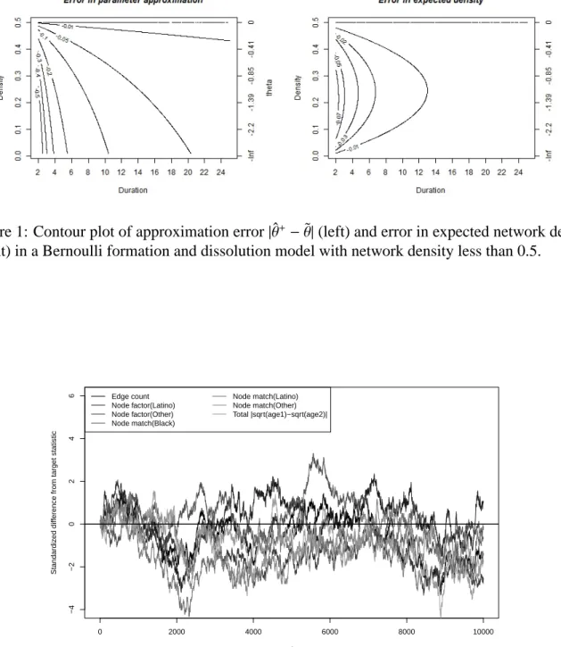
Figure 3 gives the mean of the differences between the approximated and estimated STERGM parameters. We see that the differences are generally largest for short duration and very high number of triangles. The former is to be expected given the asymptotic nature of our results, and the latter indicates that models that depart more from relational independence are indeed less well fit by the approximation methods. In general, the magnitudes of the differences for edges and degree terms are under 0.2 for models with at least moderate duration, regardless of the target number of triangles. The GWESP term exhibits differences of a larger magnitude when duration is short and the number of triangles is extreme.
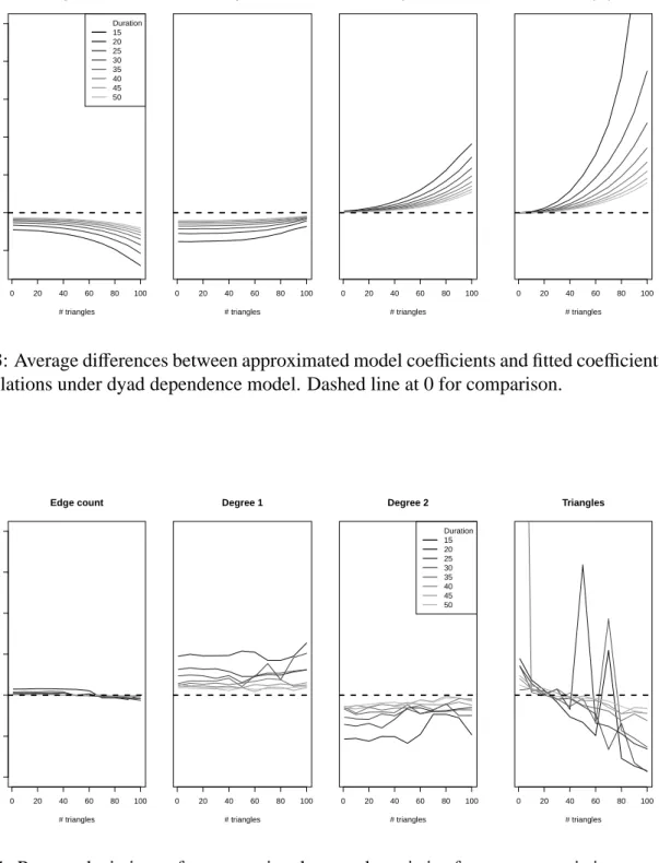
The question remains, however, whether the observed differences are large enough to impact the characteristics of networks simulated from the model, which can be used either as a measure of goodness-of-fit of the model or for simulation studies. To examine this, we simulated networks for 5000 time steps from a randomly selected vector of the approximated parameter estimates. Figure 4 shows the percent difference between the mean network statistics from the last 4000 time steps (the first 1000 were discarded as burn-in) and the target statistics for each network.
We can see that the bias in the cross-sectional network statistics decreases consistently with longer duration, regardless of the number of triangles, as we would expect given the asymptotic results for dyad independence models. On the other dimension, the bias in the number of triangles is more noisy, but shows a clear trend toward increasing downward bias as the number of triangles increases. Thus, the approximation can be quite bad for short durations, but for the majority of
would have durations even as short as those we use in this simulation, and often much longer, making it more likely that the use of the approximation method will be satisfactory.
In a case where the approximation is not statisfactory, however, using the estimates from the approximation results in radically improved fitting time for the STERGM. For example, in an analogous case to these simulations with a mean duration of 5 time steps and just one triangle, we see that the simulated network statistics using the approximated values are offby 10–30%, so we would likely not want to use the approximation itself as our parameter estimates. If we run a traditional STERGM estimation approach for this case, it takes over five hours to complete the fitting process. If, however, we use the approximated values as the starting point for the fitting algorithm, the fit completes in 1.7 minutes.
5.1
Application: Modeling the spread of HIV among MSM in the US,
revis-ited
In Section 4.2, we demonstrated the use of the adjustment to the static ERGM fit as model param-eters in a relational independence model. In reality, the degree distribution is of vital importance when modeling sexual networks, particularly when modeling the spread of disease over said net-works. We would like to add a term for the number of men in two simultaneous relationships to control for the tendency for or against forming concurrent partnerships.
The new formation model is then given by
PrY+= y+|Yt−1;θ+∝ θ+(e)∙e+X r θ+(u r)∙ur+ X r θ+(m r)∙mr+θ+(d2)∙d2 +θ+(a)X k<l |(page(k)− page(l))|+X c=r,i θ+(m c)∙mc,
where we have added a term d2=the number of actors in exactly two main partnerships at a given
time. Note that this is a dyad dependent term. The model also enforces a constraint of no more than two main partnerships at a time, another form of dependence.
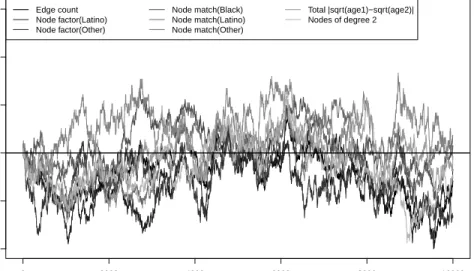
from their target values over the evolution of the network for 10,000 time steps using the relational dependence model. The parameter values used for network simulation here are those given by the approximation to the full dynamic model fit given in Section 4.1. In this case, the simulated network including the dyad dependent degree 2 term has fewer extreme deviations from the target statistics than were observed in the dyad independence case. This should not be over-interpreted, since each simulation is only one realization of a stochastic process. We can say, however, that the network evolution over time is consistent with the cross-sectional data used to generate the target network statistics when using the approximation in place of a full dynamic model fit.
6
Conclusion
This paper introduces a useful approximation method to generate estimates of the STERGM dy-namic model parameters that is much less computationally intensive than the full algorithm used for estimation in the dynamic model, when modeling cross-sectional or egocentric network data with independent data on the duration of relationships. Using this type of data to model network evolution requires an assumption that the stochastic process driving network evolution has reached a stationary distribution. It would be inappropriate, therefore, in a situation where the underlying rules of the stochastic process are changing, such as in the midst of an intervention on network attributes (e.g., rate of partner change), or where marginal distributions of network statistics are changing (because the process has not yet reached equilibrium).
We assume that dissolution parameters are fixed as a function of the average durations of re-lationships, and approximate the STERGM formation parameters by subtracting these dissolution parameters from the corresponding elements of the vector of parameter estimates obtained by esti-mating the formation model with a cross-sectional ERGM. Even in cases where the approximation itself is inadequate as an estimator, using the approximation estimates as a starting point for the algorithm greatly increases the likelihood of convergence in the estimation procedure. This ap-proach is implemented in the tergm package for modeling dynamic networks in the statnet suite of packages.
The proofs given in this paper assume relational independence models and that the model terms are categorical. However, network modelers, and particularly those using ERGMs, are typically most interested in cases that involve relational dependence, as these are the instances in which an explicit network approach has the most to offer over other frameworks. We were prevented from obtaining tractable proofs in the case of models with relational dependence either within or be-tween time steps, wherein the stationary distribution can only being defined recursively. However, as we see in the examples, the approximation works well even for non-categorical terms and de-pendence models in many cases, under the same conditions as when it worked well for categorical and independence models (long durations, small density). This holds true as well in the many additional cases that we have explored in practice, which have used a wider array of dependence terms than those we show in this paper. We thus hope that this work will serve as a starting point for further theoretical and empirical exploration of this method.
The asymptotic nature of the results suggests that they are most useful for duration sufficiently long and density sufficiently small. In one sense, it is quite easy to deal with the issue of duration; since duration here refers to MCMC steps, we could in theory rescale the relational duration so that one MCMC step equals an arbitrarily small unit of real time. Since θ− andθ+ must balance
each other to maintain the density and other targeted features of the network, this will be limited in reality to a range where θ+ does not approach −∞, however the assumptions necessary for
the approximation should be satisfied well before this level of resolution in time is reached. An additional advantage of equating an MCMC step to a small unit of time is improved plausibility of the assumption of separability of the formation and dissolution processes within MCMC steps. This poses computational difficulties, however, if the model is to be used to simulate dynamically evolving networks, as it increases the number of simulation steps needed to produce a particular duration proportionately. In some cases, such as the example used in the application, there may be an external reason why equating an MCMC step to a particular time unit is necessary. Given the likelihood of computational or other constraints, further work is needed to ascertain in exactly which cases it is appropriate to use the approximation method, and when it is advisable to fit the STERGM.
As we demonstrate in the HIV modeling examples, it is important when using this approxima-tion to perform model diagnostics by simulating one or more dynamic networks from the model parameters and checking to see that the cross-sectional network statistics are varying stochastically about the target statistics. Doing so is a minimum check that the approximation has adequately captured the sufficient statistics that a full estimation would be guaranteed to capture, and does not preclude additional diagnostics to assess model fit, e.g. those in Hunter et al. (2008a). This check is particularly important if one wishes to use the approximation as a final parameter estimate instead of merely a starting point for a full dynamic model fit.
The initial development of ERGMs offered enormous promise as a generalized framework for the statistical modeling of cross-sectional social networks. However, years of research and de-velopment were needed to identify and overcome a variety of issues to ensure that their practical application lived up to this promise. The recently proposed STERGM class of models offers sim-ilar promise for dynamic social networks. Since STERGMs build upon ERGMs, there is reason to hope that most of the issues that will arise in their application will parallel those that have al-ready been investigated, and thus will be quick to resolve. At least one new issue has alal-ready arisen, however—the particularly high computational burden needed to fit these models under cer-tain conditions—which this paper explains and then identifies a solution to. We hope that resolving this issue will position STERGMs to be of as great general applicability and usefulness as ERGMs have proven. Our concurrent and successful application of STERGMs in a number of ongoing re-search projects, made possible by the work laid out in the paper, suggest to us that this will indeed be the case.
Acknowledgments
This work is supported by NIH grants R01–GM083603, R01–HD068395, and R01–AI083060. We are grateful to Martina Morris, Skye Bender-deMoll, and the rest of the University of Washington network modeling team for helpful discussions.
References
Aral, S., Muchnik, L., and Sundararajan, A. (2009). Distinguishing influence-based contagion from homophily-driven diffusion in dynamic networks. Proceedings of the National Academy of
Sciences of the United States of America, 106(51):21544–21549.
Doreian, P. and Stokman, F. N., editors (1997). Evolution of social networks. Routledge.
Frank, O. (1991). Statistical analysis of change in networks. Statistica Neerlandica, 45(3):283– 293.
Frank, O. and Strauss, D. (1986). Markov graphs. Journal of the american Statistical association, 81(395):832–842.
Goodreau, S., Cassels, S., Kasprzyk, D., Montao, D., Greek, A., and Morris, M. (2010). Concur-rent partnerships, acute infection and hiv epidemic dynamics among young adults in zimbabwe.
AIDS and Behavior, pages 1–11. 10.1007/s10461-010-9858-x.
Goodreau, S. M., Carnegie, N. B., Vittinghoff, E., Lama, J. R., Sanchez, J., Grinsztejn, B., Koblin, B. A., Mayer, K. H., and Buchbinder, S. P. (2012). What drives the US and Peruvian HIV epidemics in men who have sex with men (MSM)? PLoS ONE, 7(11):e50522.
Goodreau, S. M., Kitts, J. A., and Morris, M. (2009). Birds of a feather, or friend of a friend? using exponential random graph models to investigate adolescent social networks. Demography, 46(1):103–125.
Hall, H. I., Song, R., Rhodes, P., Prejean, J., An, Q., Lee, L. M., Karon, J., Brookmeyer, R., Kaplan, E. H., McKenna, M. T., and Janssen, R. S. (2008). Estimation of HIV incidence in the United States. JAMA, 300(5):520–529.
Handcock, M. S., Hunter, D. R., Butts, C. T., Goodreau, S. M., and Morris, M. (2008). statnet: Software tools for the representation, visualization, analysis and simulation of network data.
Hanneke, S., Fu, W., and Xing, E. P. (2010). Discrete temporal models of social networks.
Elec-troninc Journal of Statistics, 4:585–605.
Holland, P. W. and Leinhardt, S. (1977). A dynamic model for social networks. Journal of
Math-ematical Sociology, 5(1):5–20.
Hummel, R. M., Hunter, D. R., and Handcock, M. S. H. (2012). Improving simulation-based algorithms for fitting ERGMs. Journal of Computational and Graphical Statistics, 21(4):920– 939.
Hunter, D. R., Goodreau, S. M., and Handcock, M. S. (2008a). Goodness of fit of social network models. Journal of the American Statistical Association, 103(481):248–258.
Hunter, D. R. and Handcock, M. S. (2006). Inference in curved exponential family models for networks. Journal of Computational and Graphical Statistics, 15(3):565–583.
Hunter, D. R., Handcock, M. S., Butts, C. T., Goodreau, S. M., and Morris, M. (2008b). ergm: A package to fit, simulate and diagnose exponential-family models for networks. Journal of
Statistical Software, 24(3):1–29.
Jack, S., Moult, S., and Anderson, A. R. (2010). An entrepreneurial network evolving: Patterns of change. International Small Business Journal, 28(4):315–337.
Krivitsky, P. N. (2012a). Modeling of dynamic networks based on egocentric data with durational information. Technical Report 2012-01, Pennsylvania State University Department of Statistics.
Krivitsky, P. N. (2012b). Modeling tie duration in ergm-based dynamic network models. Technical Report 2012-02, Pennsylvania State University Department of Statistics.
Krivitsky, P. N. and Handcock, M. S. (2012). A separable model for dynamic networks. Journal
of the Royal Statistical Society: Series B.
Krivitsky, P. N., Handcock, M. S., and Morris, M. (2011). Adjusting for network size and composi-tion effects in exponential family random graph models. Statistical Methodology, 8(4):319–339.
Mercken, L., Snijders, T. A., Steglich, C., and de Vries, H. (2009). Dynamics of adolescent friendship networks and smoking behavior: Social network analyses in six european countries.
Social Science and Medicine, 69(10):1506–1514.
Morris, M. and Kretzschmar, M. (2000). A microsimulation study of the effect of concurrent partnerships on the spread of HIV in Uganda. Mathematical Population Studies, 8(2):109–133.
Morris, M., Kurth, A. E., Hamilton, D. T., Moody, J., and Wakefield, S. (2009). Concurrent partnerships and HIV prevalence disparities by race: Linking science and public health practice.
American Journal of Public Health, 99:1023–1031.
Prejean, J., Song, R., Hernandez, A., Ziebell, R., Green, T., Walker, F., Lin, L. S., An, Q., Mermin, J., Lansky, A., Hall, H. I., and HIV Incidence Surveillance Group, . (2011). Estimated HIV incidence in the United States, 2006-?2009. PLoS ONE, 6(8):e17502.
R Development Core Team (2011). R: A Language and Environment for Statistical Computing. R Foundation for Statistical Computing, Vienna, Austria. ISBN 3-900051-07-0.
Robins, G. and Morris, M. (2007). Advances in exponential random graph (p*) models. Social
Networks, 29(2):169–172.
Robins, G. and Pattison, P. (2001). Random graph models for temporal processes in social net-works. Journal of Mathematical Sociology, 25(1):5–41.
Robins, G., Snijders, T., Wang, P., Handcock, M., and Pattison, P. (2007). Recent developments in exponential random graph (p*) models for social networks. Social Networks, 29(2):192–215.
Runger, G. and Wasserman, S. (1980). Longitudinal analysis of friendship networks. Social
Networks, 2(2):143–154.
Sasovova, Z., Mehra, A., Borgatti, S. R., and Schippers, M. C. (2010). Network churn: The effects of self-monitoring personality on brokerage dynamics. Administrative Science Quarterly, 55(4):639–670.
Snijders, T. and Koskinen, J. (2013). Longitudinal models. In Lusher, D., Koskinen, J., and Robins, G., editors, Exponential Random Graph Models for Social Networks, pages 130–140. Cambridge University Press, Cambridge.
Snijders, T. A. (2001). The statistical evaluation of social network dynamics. Sociological
Method-ology, 31(1):361–395.
Snijders, T. A., Pattison, P. E., Robins, G. L., and Handcock, M. S. (2006). New specifications for exponential random graph models. Sociological Methodology, 36(1):99–153.
Snijders, T. A., Steglich, C., and Schweinberger, M. (2007). Modeling the co-evolution of networks and behavior. In Van Montfort, K., Oud, H., and Satorra, A., editors, Longitudinal models in the
behavioral and related sciences, pages 41–71. Lawrence Erlbaum, Mahwah, NJ.
Strauss, D. and Ikeda, M. (1990). Pseudolikelihood estimation for social networks. Journal of the
American Statistical Association, 85(409):204–212.
Wasserman, S. (1980). Analyzing social networks as stochastic processes. Journal of the American
Statistical Association, 75(370):280–294.
Wasserman, S. and Pattison, P. (1996). Logit models and logistic regressions for social networks. I. An introduction to Markov graphs and p*. Psychometrika, 60:401–425.
Weerman, F. M. (2011). Delinquent peers in context: A longitudinal network analysis of selection and influence effects. Criminology, 49(1):253–286.
Figure 1: Contour plot of approximation error|θˆ+−θ˜|(left) and error in expected network density
(right) in a Bernoulli formation and dissolution model with network density less than 0.5.
0 2000 4000 6000 8000 10000 −4 −2 0 2 4 6 Index Standardiz ed diff
erence from target statistic
Edge count Node factor(Latino) Node factor(Other) Node match(Black) Node match(Latino) Node match(Other) Total |sqrt(age1)−sqrt(age2)|
Figure 2: Standardized deviations of cross-sectional network statistics from target statistics over 10,000 time steps under dyad independence model.
0 20 40 60 80 100 −0.2 0.0 0.2 0.4 0.6 0.8 1.0 Edge count # triangles Diff erence Duration 15 20 25 30 35 40 45 50 0 20 40 60 80 100 Degree 1 # triangles 0 20 40 60 80 100 Degree 2 # triangles 0 20 40 60 80 100 GWESP(0.5) # triangles
Figure 3: Average differences between approximated model coefficients and fitted coefficients over 50 simulations under dyad dependence model. Dashed line at 0 for comparison.
0 20 40 60 80 100 −0.10 −0.05 0.00 0.05 0.10 0.15 0.20 Edge count # triangles Diff erence 0 20 40 60 80 100 Degree 1 # triangles 0 20 40 60 80 100 Degree 2 # triangles Duration 15 20 25 30 35 40 45 50 0 20 40 60 80 100 Triangles # triangles
Figure 4: Percent deviations of cross-sectional network statistics from target statistics over 4,000 time steps under dyad dependence model. Dashed line at 0 for comparison.
0 2000 4000 6000 8000 10000 −4 −2 0 2 4 6 Index Standardiz ed diff
erence from target statistic
Edge count Node factor(Latino) Node factor(Other) Node match(Black) Node match(Latino) Node match(Other) Total |sqrt(age1)−sqrt(age2)| Nodes of degree 2
Figure 5: Standardized deviations of cross-sectional network statistics from target statistics over 10,000 time steps under dyad dependence model.