Backtesting Expected Shortfall via Multi-Quantile Regression

HAL Id: halshs-01909375

https://halshs.archives-ouvertes.fr/halshs-01909375v3

Submitted on 28 Nov 2019

HAL is a multi-disciplinary open access archive for the deposit and dissemination of sci-entific research documents, whether they are pub-lished or not. The documents may come from teaching and research institutions in France or abroad, or from public or private research centers.

L’archive ouverte pluridisciplinaire HAL, est destinée au dépôt et à la diffusion de documents scientifiques de niveau recherche, publiés ou non, émanant des établissements d’enseignement et de recherche français ou étrangers, des laboratoires publics ou privés.

Backtesting Expected Shortfall via Multi-Quantile

Regression

Ophélie Couperier, Jérémy Leymarie

To cite this version:

Ophélie Couperier, Jérémy Leymarie. Backtesting Expected Shortfall via Multi-Quantile Regression. 2019. �halshs-01909375v3�

Backtesting Expected Shortfall

via Multi-Quantile Regression

Ophélie Couperier

Jérémy Leymarie

November 28, 2019

Abstract

In this article, we propose a new approach to backtest Expected Shortfall (ES) ex-ploiting the definition of ES as a function of Value-at-Risk (VaR). Our methodology examines jointly the validity of the VaR forecasts along the tail distribution of the risk model, and encompasses the Basel Committee recommendation of verifying quantiles

at risk levels 97.5%, and 99%. We introduce four easy-to-use backtests in which we

regress the ex-post losses on the VaR forecasts in a multi-quantile regression model, and test the resulting parameter estimates. Monte-Carlo simulations show that our tests are powerful to detect various model misspecifications. We apply our backtests on S&P500 returns over the period 2007-2012. Our tests clearly identify misleading ES forecasts in this period of financial turmoil. Empirical results also show that the detection abilities are higher when the evaluation procedure involves more than two quantiles, which should accordingly be taken into account in the current regulatory guidelines.

Keywords: Banking regulation; Financial risk management; Forecast evaluation;

Hypoth-esis testing; Tail risk.

JEL classification: C12, C52, G18, G28, G32

∗_{Ensae (CREST, UMR CNRS 9194), 5 avenue Henry Le Chatelier, 91120 Palaiseau, France. Email:}

[email protected]

†_{University of Orléans (LEO, FRE CNRS 2014), 11 rue de Blois, 45067 Orléans, France. Email:}

1

Introduction

In response to the market failures revealed by the global 2007-2008 financial crisis, the Basel Committee on Banking Supervision (BCBS) has adopted the Basel III accords to improve the banking sector’s ability to absorb shocks arising from financial and economic stress (BCBS, 2010). Among the number of fundamental reforms that must be implemented until January 1st, 2022 (BCBS, 2019), the BCBS has substituted Value-at-Risk (VaR) by Expected Shortfall (ES) for the calculation of market risk capital requirements. Expected Shortfall, also referred to as Conditional VaR (CVaR) or Tail VaR (TVaR), measures the expected loss incurred on an asset portfolio given that the loss exceeds VaR. That is, if Ltis

the (integrable) ex-post loss on a portfolio at time t, Ωt−1 is the information at time t−1,

and QLt(.) is the quantile function of Lt, the τ-level ES and VaR are given by

ESt(τ) =E[Lt | Lt≥V aRt(τ) ; Ωt−1],

V aRt(τ) = QLt(τ; Ωt−1).

As an alternative tail risk measure, ES offers a number of appealing properties that overcomes the deficiencies of the more-familiar VaR. In particular, ES is coherent meaning that it satisfies the properties of monotonicity, sub-additivity, homogeneity, and translational invariance (see Artzner et al., 1999; Acerbi and Tasche, 2002). Furthermore, ES provides information about the expected size of the potential loss given that a loss bigger than VaR is experienced, while VaR only captures the likelihood of an incurred loss, and tells us nothing about tail sensitivity. In its revised standards for market risk, the BCBS emphasizes the important role of ES in place of VaR "to ensure a more prudent capture of "tail risk" and

capital adequacy during periods of significant financial market stress" (BCBS, 2016, page 1).

Although ES is now considered as the new standard for risk management and regulatory requirements, there are still outstanding questions about the modeling of ES (see e.g. Taylor,

2019; Patton et al., 2019), and the validation of the ES forecasts, or backtesting. Jorion (2006) defines backtesting as a formal statistical framework that consists in verifying if actual losses are in line with projected losses. Because ES is unobservable, its evaluation cannot be performed conventionally as a direct comparison of the observed value with its forecast, and thus generally relies on the elicitability property. A risk measure is said to be

elicitable if there exists a loss function such that the solution of minimizing the expected

loss is the risk measure itself. However, it has been established that, in contrast to VaR, ES does not meet the general property of elicitability (Gneiting, 2011), but satisfies narrower properties such as conditional elicitability (Emmer et al., 2015), or joint elicitability with VaR (Acerbi and Szekely, 2014; Fissler and Ziegel, 2016), making its evaluation trickier than VaR in practice. Several contributions are tied to these properties, and provide backtests by making explicit reference of the ES forecasts in the testing procedure (McNeil and Frey, 2000; Acerbi and Szekely, 2014; Nolde and Ziegel, 2017; Bayer and Dimitriadis, 2019).

To circumvent the lack of elicitability of ES, several alternative testing strategies have been proposed in the literature. Following the recent classification of Kratz et al. (2018), these backtests enter the category ofimplicit backtests, as they focus on the tail distribution characteristics of the model rather than directly on ES. They generally exploit the fact that ES can be expressed as a function of VaR, which itself is elicitable. Assume the law of Lt

is continuous. Definition of a conditional probability and a change of variable yield a useful representation of ES in terms of VaR

ESt(τ) = 1 1−τ Z 1 τ V aRt(u)du. (1)

Based on this analogy, Costanzino and Curran (2015) derive a coverage backtest for spectral risk measures such as ES in the spirit of the traditional VaR coverage backtests. Du and Escanciano (2017) define a cumulative violation process for ES that generalizes the violation

process for VaR and propose two backtests of ES. Starting with the same process, Löser et al. (2019) develop a backtest of ES that is theoretically valid in finite out-of-sample size and that can be easily extended to a multivariate setting. Costanzino and Curran (2018) provide a Trafic Light backtest for ES which extends the so-called Traffic Light backtest for VaR. More largely, several additional techniques have been proposed to assess the whole return distribution encompassing ES as a special case (Berkowitz, 2001; Kerkhof and Melenberg, 2004; Wong, 2008). See the survey of Argyropoulos and Panopoulou (2016) for more details. In this article, we also propose to exploit the relationship that prevails between ES and VaR, but contrary to the existing literature, our procedure aims at focusing on a finite number of VaRs. Definition of a Riemann sum gives a handy approximation of ES,

ESt(τ)≈ 1 p p X j=1 V aRt(uj),

where the risk leveluj is defined byuj =τ+(j−1)1−_pτ forj = 1,2, . . . , p. This representation

suggests that p quantiles with appropriate risk levels would be convenient to assess the performance of an ES model. In other words, an estimate/forecast ofESt(τ) issued from a

given model could be considered valid if the sequence ofV aRt(uj) estimates/forecasts issued

from the same model is itself valid. This testing strategy is fully consistent with the general recommendation of financial supervisors, indicating that "Backtesting requirements [for ES] are based on comparing each desk’s 1-day static value-at-risk measure [...] at both the 97.5th

percentile and the 99th percentile" (BCBS, 2016, page 57).

The main contribution of this article is to propose an original backtesting methodology to ES based on the theory of multi-quantile regression. We develop a multivariate framework, focusing on multi-quantile regression, to jointly assess VaR at multiple levels in the tail distribution of the risk model. The method extends the seminal idea of Gaglianone et al. (2011) to evaluate the validity of a single VaR relying on a single quantile regression.

Our backtesting procedure has many advantages. First, our approach encompasses the regulatory standards that consist of verifying the validity of two given quantiles. Second, our validation strategy offers flexibility since the risk manager or the supervisor may select both the number of risk levels and their magnitude depending on the objective in mind (regulatory guidelines, ES statistical approximation, etc.). Third, our testing strategy enters the category of regression-based backtests and complements the existing literature on regression-based risk forecast evaluation (see Engle and Manganelli, 2004; Christoffersen, 2011; Bayer and Dimitriadis, 2019, among others). Finally, our approach represents an alternative to the multiple VaR exceptions backtests (see Colletaz et al., 2013; Kratz et al., 2018).

Formally, we show that the parameters of the multi-quantile regression model have spe-cific properties under the hypothesis of valid ES forecasts. We propose four backtests which correspond to various linear restrictions on these parameters. These restrictions are im-plications of a Mincer-Zarnowitz representation (Mincer and Zarnowitz, 1969). Then, we test the resulting parameter restrictions using Wald-type inference. Finally, we introduce a procedure deduced from our regression framework to adjust the invalid risk forecasts.

Several approaches to estimation and statistical inference in multi-quantile regression are suggested. Our baseline procedure is to apply the QML estimation method (White et al., 2008, 2015), and then, to implement a pairs bootstrap algorithm (Freedman, 1981) in order to correct the finite sample size distortions of our backtests. A second approach is to consider the estimation method of Jun and Pinkse (2009) which is designed to improve estimation efficiency in presence of correlated generalized errors and to apply the pairs bootstrap. An ultimate approach, although only available for single quantile models, consists of applying the procedure of Chernozhukov and Fernández-Val (2011) based on the extreme value theory. Several Monte Carlo experiments are provided and an empirical application with the S&P500 series is conducted. Our backtests deliver good performances to detect misleading

ES forecasts. We also find that the use of asymptotic critical values is prone to substantial size distortions, while the implementation of bootstrap critical values provides satisfactory size performances regardless of the sample size. The latter should hence be preferred when asymptotic theory does not apply conveniently.

Our empirical results suggest an update of the regulatory guidelines. First, we show that the BCBS recommendation of assessing quantiles at risk levels 97.5% and 99% is not always sufficient to identify misspecified ES models. The use of additional quantiles is recommended to improve the soundness of the decision. Second, our results suggest to limit the number

p of quantiles in small samples (with typically p ≤ 6) and to consider higher values if the historical sample covers longer periods. Finally, we show numerically that our approximation of ES as a combination of several VaRs is close to its theoretical counterpart, which strongly supports its implementation in a risk management viewpoint.

The rest of the paper is organized as follows. In Section 2, we introduce the multi-quantile regression framework. Section 3 describes the null hypotheses of our tests, the test statistics, their asymptotic properties, and the procedure to implement the bootstrap critical values. Section 4 examines the finite sample performance of the proposed backtests through a set of Monte Carlo experiments. In Section 5, we apply our backtesting methodology on the S&P500 index and introduce the procedure to adjust the imperfect ES forecasts. This section also contains a number of robustness checks with alternative estimation and statistical inference approaches. Finally, we conclude the paper in Section 6.

2

Multi-quantile regression framework

This section describes our proposed multi-quantile regression approach. In the first part, we discuss the usefulness of approximating ES via a finite sum of VaRs. In a second part, we describe the multi-quantile regression model that we employ in our testing strategy. The

last part is devoted to the description of the estimation method and the asymptotic theory.

2.1

ES as an approximation of VaRs

Our backtesting procedure exploits the relationship between VaR and ES. We suppose that ES can be approximated as an average of VaRs. This assertion stems from the representation of ES as the limit of a Riemann sum when the partition becomes infinitely fine.

Definition 1 (ES approximation). Let τ ∈ ]0,1[ denote the coverage level. The τ-level ES

approximation is defined as a finite Riemann sum involving p VaRs such as

ESt(τ)≈ 1 p p X j=1 V aRt(uj), (2)

where risk levels uj, j = 1,2, . . . , p, satisfy uj = τ + (j−1)1−_pτ, and p denotes the number

of subdivisions taken in the definite integral.

Our approximation of ES averages VaRs in the upper tail distribution of the risk model. The number of quantiles involved in the sum is given bypand characterizes the approxima-tion accuracy. In particular,p= 1 involves a single VaR at coverage levelτ, while increasing

p to infinity leads Equation (2) to converge to the theoretical ES. As we rely on a Riemann sum, the approximation assigns equal weights 1/pto each element in the sum, and the risk levels uj, j = 1,2, . . . , p, are determined so that the interval is equally partitioned between

the two boundariesτ and 1. Several alternatives for the approximation of a definite integral are available. Here, we rely on a Riemann sum for its simplicity and ease of implementation. We show how to derive the above formula in Appendix A.

In practice, pmay be chosen small as the interval of the definite integral is restricted to the extreme upper tail distribution. For instance, Gouriéroux and Liu (2012) identify for a large class of distributions a common linear conversion pattern between VaR and ES, so that a few VaRs are generally enough to get a good approximation of ES. Daníelsson and Zhou

(2016) empirically show that VaR and ES are in most cases related by a small constant and are hence almost equally informative. Kratz et al. (2018) provide multinomial backtests of VaRs, and show that backtesting exceptions jointly at four to eight risk levels yields a very effective test in terms of balancing simplicity and reasonable size and power properties.

Our approximation is useful for at least two reasons. First, this simple formula is ap-pealing in a regulatory and risk management viewpoint since the estimation of VaR is well-established and its computation is easier compared to ES. Secondly, and it is the purpose of this paper, the above relationship greatly simplifies the assessment of ES, by focusing on the validity of several VaRs, and is more intelligible in the context of banking regulation. This approach is fully consistent with the BCBS guidelines on ES assessment stating that " Back-testing requirements [for ES] are based on comparing each desk’s 1-day static value-at-risk

measure [...] at both the 97.5th percentile and the 99th percentile" (BCBS, 2016, page 11).

2.2

Multi-quantile regression model

In the sequel, we consider an asset or a portfolio, and denote by Lt the corresponding loss

observed at time t, for t = 1,2, . . . , T. In addition, we denote by Ωt−1 the information set

available at time t−1, with (Lt−1, Lt−2, . . .)⊆Ωt−1. Formally, the Ωt−1 conditional VaR at

level uj of the Lt distribution is the quantity V aRt(uj) such that

Pr (Lt≥V aRt(uj)|Ωt−1) =uj. (3)

A VaR model is said to be correctly specified (at coverage level uj) as soon as Equation (3)

holds for all t. In practice, VaR forecasts are assessed through the evaluation of this simple equality. Given the ES approximation introduced in Definition 1, this equality may arguably be adapted for the assessment of ES models. The chief insight is to evaluate Equation (3) for a number pof risk levels as set out in Definition 1. Accordingly, one should conclude to the appropriateness of a given ES model as soon as the sequence V aRt(uj), t= 1,2, . . . , T,

issued by the ES model satisfies Equation (3) jointly for j = 1,2, . . . , p.

We refer to the original idea of Gaglianone et al. (2011) who derive a backtest of VaR at a single coverage level, introducing VaR as a regressor of a quantile regression model. We generalize their approach for the assessment of multiple VaRs. To do so, we regress the ex-post losses {Lt, t = 1,2, . . . , T} on the p VaR forecasts {V aRt(uj), t = 1,2, . . . , T}j=1,2,...,p

in a multi-quantile regression model.

Lt=β0(uj) +β1(uj)V aRt(uj) +j,t ∀j = 1,2, . . . , p, (4)

whereβ0(uj), andβ1(uj), respectively, denote the intercept and the slope parameters at level

uj, and wherej,t is the error term at risk leveluj and time t, such that theuj-th conditional

quantile ofj,t satisfiesQj,t(uj; Ωt−1) = 0. This specification could be interpreted as a

multi-quantile regression version of Koenker and Xiao (2002). More specifically, the representation is tightly related to the multi-quantile CaViAR model (MQ-CaViAR) of White et al. (2008, 2015) which allows a joint modeling of multiple conditional VaRs. Given the multi-quantile regression model of Equation (4), the uj-th conditional quantile of Lt is defined as

QLt(uj; Ωt−1) =β0(uj) +β1(uj)V aRt(uj) ∀ j = 1,2, . . . , p. (5)

This equation is central for our backtesting methodology as it establishes a direct link be-tween the VaR forecasts (issued from the external ES model), with the true unknown condi-tional quantile (issued from the ex-post observed losses). Our procedure consists in verifying if there exists a perfect match between V aRt(uj) and QLt(uj; Ωt−1). Consistently with

Gaglianone et al. (2011), we rely on the regression parameters, and test if the intercept parameter β0(uj), and the slope parameterβ1(uj), are respectively equal to zero, and one,

for j = 1,2, . . . , p. For these values, and given Definition 1, the risk model is accepted as a valid proxy of the true unknown data generating process to deliver the ES forecasts.

2.3

Parameter estimation and asymptotic properties

Our backtesting procedure requires to consistently estimate the parameters β0(uj), and

β1(uj), for j = 1,2, . . . , p. Under the hypothesis that a sequence of VaR is valid, coefficients

satisfy β0(uj) = 0, and β1(uj) = 1, for j = 1,2, . . . , p. In what follows, we denote by

β(uj) = (β0(uj), β1(uj))

0

the vector of parameters for the uj-th quantile index, and we

write β = β(u1) 0 , β(u2) 0 , . . . , β(up) 00

the stacked vector of 2p coefficients. We assume that the sequence {uj, j = 1,2, . . . , p} is ordered in the sense that u1 < u2 < . . . < up <1.

In order to estimate β, we consider the QML estimator proposed by White et al. (2008, 2015) dedicated to multi-quantile regression, given by

b β =arg min β∈R2p T −1 T X t=1   p X j=1 ρuj(Lt−β0(uj)−β1(uj)V aRt(uj))  ,

whereρuj(x) =xψuj(x) is the standard "check function", andψuj(x) = uj−1(x≤0) is the

usual quantile step function. Under suitable regularity conditions, White et al. (2008, 2015) show that this estimator is consistent and asymptotically normally distributed. The condi-tions are described in Appendix B and a discussion is provided on how these assumpcondi-tions are fulfilled in our context. However, in case of correlated generalized errors ψ(j,t) between

different quantiles, the QML estimator is not necessarily efficient. The procedure of Jun and Pinkse (2009) is designed to improve efficiency in the presence of dependent cross-equation errors. An application to this procedure is provided in Section 5.2 to gauge potential interest. Under Assumptions A0-A2 in Appendix B, the asymptotic distribution of the QML estimator is given by

√

T βb−β _d

→ N(0,Σ),

where Σ denotes the asymptotic covariance matrix which takes the form of a Huber (1967) sandwich. Its expression is given by Σ = A−1V A−1, with V = E[ηtηt0], ηt =

Pp j=1∇QLt(uj; Ωt−1)ψuj(j,t), A = Pp j=1E[fj,t(0)∇QLt(uj; Ωt−1)∇ 0_Q Lt(uj; Ωt−1)], where

∇QLt(uj; Ωt−1) denotes the 2p gradient vector differentiated with respect to β, j,t =

Lt−QLt(uj; Ωt−1), and fj,t(0) denotes the pdf of j,t evaluated at zero. In Appendix C,

we provide a consistent estimator Σ of Σ that will be used to compute our test statistics.b

Finally, Appendix D provides a discussion on the rate of convergence and interplay of

p and T when T tends to infinity. Under this asymptotic framework, we show that p is increasing with T. Then, we consider a simple illustration assuming p takes the form of a power function. Under this assumption, T needs to diverge faster than p to preserve the asymptotic theory of White et al. (2008, 2015). This condition is not importantly restrictive but suggests the existence of an (asymptotic) upper limit for pwhich depends on the sample size. Section 4 provides several Monte-Carlo experiments with various values for pand T to give guidelines on how to choose these parameters jointly in finite samples.

3

Backtesting ES

In this section, we present our backtests for ES. Our procedures assess whether the parame-ters β0(uj) and β1(uj) coincide with their expected values for risk levels uj, j = 1,2, . . . , p.

To this end, we propose four backtests that analyze various settings on the regression co-efficients. In the sequel, we introduce the null hypotheses, the test statistics, and establish their asymptotic properties. Finally, we discuss the use of finite sample critical values and provide a bootstrap algorithm when the asymptotic theory does not apply conveniently.

3.1

The backtests

Formally, our goal is to test β0(uj) = 0, and β1(uj) = 1, for j = 1,2, . . . , p. As highlighted

by Gaglianone et al. (2011) for a unique quantile regression, the aforementioned set of re-strictions retains a Mincer and Zarnowitz (1969) interpretation for each quantile regression in (4). Here, we propose to test various implications of these coefficient restrictions by taking

into consideration four distinct null hypotheses based on a reduced number of constraints. Many backtests test implications of a more general hypothesis. In this context, Du and Escanciano (2017) assess two implications for the martingale difference sequence of their cumulative violation process. McNeil and Frey (2000) and Nolde and Ziegel (2017) propose to test the zero mean hypothesis of their residuals which more largely behave as white noise.

Definition 2 (Null hypotheses). Denote by J1, J2, I, and S, the four backtests. The

corre-sponding null hypotheses H0,J1, H0,J2, H0,I, H0,S, are defined as follows:

H0,J1 : p X j=1 (β0(uj) +β1(uj)) =p, (6) H0,J2 : p X j=1 β0(uj) = 0, and, p X j=1 β1(uj) =p, (7) H0,I : p X j=1 β0(uj) = 0, (8) H0,S : p X j=1 β1(uj) = p, (9)

where notations J1 and J2 indicate the "joint" backtests, and where I and S refer to the

"intercept" backtest and to the "slope" backtest, respectively.

Equations (6)-(9) of Definition 2 gives the null hypotheses H0,J1,H0,J2,H0,I,H0,S. They

are devised to assess various implications that the regression coefficients should satisfy when the ES forecasts are valid. The coefficients are summed across risk levelsuj, j = 1,2, . . . , p.

This aggregation substantially reduces the number of constraints. H0,J2 is hence

charac-terized by two constraints, and H0,J1, H0,I, H0,S involve a single constraint. Furthermore,

aggregating coefficients along the quantile curve allows addressing the quantile crossing prob-lem that appears when multiple quantiles are jointly estimated. As stressed by Chernozhukov et al. (2010), quantile crossing is a problem when the ultimate goal of a researcher is model-ing the quantile curve. Alternately our testmodel-ing procedure focuses on the parameter estimates of the quantile models. As the procedure of Chernozhukov et al. (2010) does not require any

re-estimation ofβ0(uj) and β1(uj), the statistics J1, J2,I,S, remain unchanged.

Our null hypotheses analyze various settings on the regression coefficients. The null of the joint backtests, H0,J1 and H0,J2, look at the expected value of both the intercept and

slope parametersβ0(uj) andβ1(uj) forj = 1,2, . . . , p. H0,J1 sums the two types of coefficient

together, while H0,J2 sums the coefficients separately depending on whether they are slope

parameters or intercept parameters. Finally, the null hypotheses of the intercept backtest and the slope backtest,H0,I andH0,S, focus solely on one of the two parameter components. H0,I

is built to examine the intercept parameters β0(uj), j = 1,2, . . . , p, and H0,S is devoted to

the analysis of the slope parametersβ1(uj),j = 1,2, . . . , p. These additional null hypotheses

complement the joint backtests to identify the nature of the misspecification. If the joint hypotheses are rejected, separate tests for these two types of measurement error should be considered. They are inspired by the prediction-realization framework of Mincer and Zarnowitz (1969). When H0,I is rejected, the intercept parameters, β0(uj), j = 1,2, . . . , p,

do not sum to 0, and hence, the average of VaR forecasts either underestimate or overestimate the true quantiles, if the sign of the sum is positive or negative, respectively. The rejection ofH0,S indicates that the sum of the slope parametersβ1(uj), j = 1,2, . . . , p, does not equal

p, which highlights correlation between the forecasting errors and the quantile series.

Definition 3(Wald-test statistics). Let us denote by W ∈ {J1, J2, I, S}the generic notation

for the test statistic, and consider the classical formulation of a Wald-type test such as H0,W:

RWβ =qW. The general expression of the test statistics is given by

W =T RWβb−q_W 0 RWΣbR0 W −1 RWβb−q_W , (10)

where T is the out-of-sample size, and Σb denotes a consistent estimator of the asymptotic

covariance matrix.

Defini-tion 3 gives the general expression of the test statistics. According to our notaDefini-tions, substitut-ingW byJ1,J2,I, andS, yields the four test statistics. For ease of presentation, the null

hy-potheses are now presented in a classical formulation, such thatH0,W :RWβ =qW. Given the

null hypotheses of Definition 2, the quantities RW and qW are as follows: RJ1 =ιp⊗

1 1, qJ1 =p, RJ2 =ιp ⊗I2, qJ2 = 0 p0, RI = ιp⊗ 1 0, qI = 0, RS =ιp ⊗ 0 1, qS =p,

where ιp is a p-row unit vector, and I2 denotes the identity matrix of size 2.

Proposition 1 (Chi-squared distribution). Consider the multi-quantile regression model in

Equation (4), Assumptions A0-A3 in Appendix B, and the null hypotheses of Definition 2,

the test statisticsJ1,I, andS, converge to a chi-squared distribution with 1 degree of freedom,

and the test statistic J2 converges to a chi-squared distribution with 2 degrees of freedom.

Proposition 1 gives the asymptotic distribution of the Wald statistics J1, J2,I, S under

their respective null hypotheses H0,J1, H0,J2, H0,I, H0,S. As a result of coefficients’

aggre-gation, the asymptotic distributions are based on a small and fixed number of degrees of freedom no matter howp is chosen. Thus, the four backtests have unchanged critical values whatever the number of quantiles considered in the ES approximation. Finally, we provide in Appendix E the proof for consistency of the tests under fixed untrue hypothesis.

3.2

Finite sample inference

Our four backtests are asymptotically chi-squared distributed and we can employ them if the asymptotic conditions are fulfill for realistic sample sizes. However, in the case of ES assessment, the focus is on the extreme tail distribution, that is for risk levels above the regulatory coverage level, i.e. τ = 0.975. This may induce scarce information and affect the inference when the sample size is not large enough. Furthermore, the asymptotic framework of White et al. (2008, 2015) implicitly assumes that (1−up)T diverges to infinity, where

Chernozhukov and Fernández-Val (2011) provide a refinement of this assumption based on the extreme value theory allowing (1−up)T →k < ∞. However, to date this literature has

only considered single quantile models and it is not obvious how the results for the single quantile models extend to multi-quantile models. To overcome these typical deficiencies, we implement a bootstrap procedure to adjust the critical values of our test statistics in finite samples.

In the following, we propose a pairs bootstrap algorithm (Freedman, 1981) in order to correct the finite sample size distortions of our backtests. This is a fully non-parametric procedure that can be applied to a very wide range of models, including quantile regression model (Koenker et al., 2018). This approach consists in resampling the data, keeping the dependent and independent variables together in pairs. The procedure is valid for any sample sizes T, and large levels uj, j = 1,2, . . . , p, and ideally applies in our case when the

constraints of the null hypothesis are linear in the parameters. The algorithm is as follows: 1. Estimateβand Σ on the original data{Lt, V aRt(uj)}j=1,2,...,p,t= 1,2, . . . , T, to obtain

b

β and Σ, and compute the unconstrained test statisticb W given by

W =T RWβb−q_W 0 RWΣbR0_W −1 RWβb−q_W .

2. Build a bootstrap sample by drawing with replacement T pairs of observations from the original data {Lt, V aRt(uj)}j=1,2,...,p,t = 1,2, . . . , T.

3. Estimate the model on the bootstrap sample, to obtain βbb and Σbb, and compute the

bootstrapped test statistic Wb under the null hypothesis as follows:

Wb =T RWβbb−R_Wβb 0 RWΣbbR0_W −1 RWβbb−R_Wβb .

4. RepeatB−1 times steps 2 and 3, to obtain the bootstrap statisticsWb,b= 1,2, . . . , B. Two remarks should be made about the algorithm. First, when we use the pairs

boot-strap we cannot impose the null hypothesis on the bootboot-strap data generating process since imposing restrictions on β is unfeasible. To overcome this issue, we calculate the bootstrap statistics by considering the differenceRWβ−RWβbrather thanR_Wβ−q. Since the estimate

of β from the bootstrap samples should, on average, be equal to βb, at least asymptotically,

the null hypothesis tested by Wb becomes "true" for the pairs bootstrap data generating process. Second, the critical valuecα is obtained as theα-quantile of the bootstrap statistics

Wb, b= 1,2, . . . , B. The decision rule is as follows. If the original test statisticW is greater than the α-level bootstrapped critical value cα, we conclude to the rejection of the null

hypothesis. In addition, we compute the p-value of the test as P =B−1PB b=11

Wb > W.

4

Simulation study

In this section, we provide Monte Carlo simulations to illustrate the finite sample properties (empirical size and power) of our four backtests. The simulation study is performed on 5000 replications, and we consider sample sizes T = 250,500,1000,2500. The results associated with the bootstrap critical values are based on B = 1000 bootstrap samples. Finally, the backtests are computed withτ = 0.975 that is the current banking regulation coverage level. Beyond the traditional size and power analysis, a second important objective of this section is to characterize the influence of the number p of quantiles used to assess the ES forecasts. We aim at examining whether an ES backtest based on a large number of quantiles may provide better performances than a backtest based on a small number of quantiles, as it is recommended by the current BCBS guidelines. For that, we consider different choices for the number of risk levels, namely p = 1,2,4,6,8,10,12. The p risk levels u1, u2, . . . , up

are computed in accordance with Definition 1. Notice that p = 1 coincides with the VaR backtest at level τ of Gaglianone et al. (2011). With p = 2 risk levels, our backtests are in accordance with the number of quantiles of the regulatory guidances. Finally, the casep= 4

corresponds to the framework considered by Emmer et al. (2015).

The correct data generating process is given by the AR(1)-GARCH(1,1) specification with Student innovations. This model has been widely used for assessing tail risk measures (see e.g. McNeil and Frey, 2000; Du and Escanciano, 2017; Löser et al., 2019, among others). The ex-post portfolio loss Lt,t = 1,2, . . . T, is given by

Lt=δ0+δ1Lt−1+t,

t=σtηt, ηt∼tv,

σ2_t =γ0+γ1t2−1+γ2σ2t−1,

(11)

wheretv denotes the Student’s t distribution withv degrees of freedom. Given the model in

Equation (11), the true ES and VaR at coverage level τ are given by

ESt(τ) =δ0+δ1Lt−1+σtm(τ), (12)

V aRt(τ) = δ0+δ1Lt−1+σtFv−1(τ), (13)

with m(τ) = E[ηt|ηt≥Fv−1(τ)], and where F

−1

v (τ) denotes the τ-quantile of the Student

distribution with v degrees of freedom. As a robustness check of the above model, Ap-pendix F provides simulation results for the simple case of a GARCH(1,1) model that excludes the conditional mean component with Lt = t where t is as in Equation (11).

Both models are calibrated using the opposite of the daily log-returns of the S&P500 index over the period from January 2, 2013 to December 29, 2017, with δb₀,δb₁,

b

γ0,γb1,γb2,vb

= (−0.085,−0.093,0.034,0.214,0.748,5) and (γb0,γb1,γb2,vb) = (0.034,0.197,0.763,5),

respec-tively for the AR(1)-GARCH(1,1) model and the GARCH(1,1) model. Finally to investigate the power, we consider several misspecified alternatives for Lt:

A1 : AR(1)-GARCH(1,1) model with underestimated conditional variances: Lt is as Equation

(11), with σ_t2 =γ0 +γ12t−1+γ2σ2t−1

A2 : GARCH in mean model: Lt =κ×σt2+t, t=σtηt, σ2t =γ0+γ12t−1+γ2σ2t−1, ηt∼tv,

where κ= +2.5,−2.5, respectively.

A3 : AR(1)-GARCH(1,1) model with mixed normal innovations: Lt satifies Equation (11), with

ηt∼

0.5X++ 0.5X−/√10, where X+ ∼ N(3,1) andX− ∼ N(−3,1).

A4 : 12-month historical simulation model : VaR and ES are given by their empirical counterparts

from the 250 previous trading days such that V aRt(τ) = percentile {Lt−i}250i=1,100τ , and ESt(τ) = 1 P250 i=11(Lt−i≥V aRt−i(τ)) 250 X i=1 Lt−i×1(Lt−i≥V aRt−i(τ)).

In A1, the conditional variance of the series σt is alternately underestimated of 25%,

50%, and 75% to examine whether our tests are able to detect an underestimation of ES stemming from a misleading appreciation of volatility. In A2, the misspecification occurs

in the conditional mean by assuming a GARCH in mean model. In A3, the distribution

of the innovations ηt is incorrect and should imply misleading ES predictions compared to

the t-distribution. Finally in scenario A4, the time-varying dynamics is incorrectly captured

by the historical simulation method. It should be noticed that our alternatives are in line with the existing literature on tail risk assessment. Bayer and Dimitriadis (2019) look at an alternative close to A1 by varying the coefficients related to the GARCH component. A2

and A3 were applied by Du and Escanciano (2017) to illustrate the performance of their

unconditional and conditional ES backtests. Finally, scenario A4 was extensively studied by

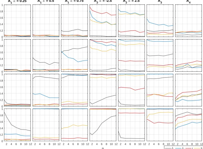
Kratz et al. (2018), Bayer and Dimitriadis (2019), Gaglianone et al. (2011), among others. Figure 1 displays graphically empirical sizes of the tests at 5% significance level. The first row reports the results of the asymptotic tests and the second row embeds those of the bootstrap based tests. Each column is for a given sample size T, and the results are shown as a function of p for comparison. As previously discussed, the use of asymptotic critical values (based on a χ2 distribution) induces important size distortions. For instance, with

Figure 1: Empirical size of the tests at 5% significance level (AR(1)-GARCH(1,1) model) 0.1 0.2 0.3 0.4 T=250 T=500 J 1 J2 I S T=1000 T=2500

Asymptotic critical values

2 4 6 8 10 12 0.04 0.06 0.08 0.1 Rejection frequencies 2 4 6 8 10 12 p 2 4 6 8 10 12 2 4 6 8 10 12

Bootstrap critical values

Note: Size of the four backtests are displayed as a function ofp. The first row reports the results computed with the asymptotic critical values, and the second row those computed with the bootstrap critical values. The columns correspond to different sample sizesT.

sample size T = 500, and p = 6, the four test statistics J1, J2, I, and S, display empirical

sizes equal to 0.126, 0.273, 0.165, 0.216, respectively. These distortions are caused by poor inference made on regression parameters in the extreme upper tail when the sample size is not sufficiently large. On the contrary, the backtests based on bootstrap critical values display empirical sizes that are close to the nominal size of 5% for all reported sample sizes and risk levels. For large coverage levels and moderate samples, we thus recommend to use bootstrap critical values rather than asymptotic ones.

In reply to questions concerning the link between p and T, we note that the size of the four bootstrap-based backtests slightly deteriorates for p > 6 with T = 250 and T = 500 revealing that the tests are sensitive to the choice ofpin small samples. In details, the slope backtest is the most affected by these distortions, while the J1 backtest is well-sized most

of the time. On the contrary, for larger sample sizes, typically T = 1000 and T = 2500, these distortions are negligible. Our recommendation is hence to restrict the number p of quantiles when applying the tests in small samples, with typically p ≤ 6, and to consider higher values if the historical sample covers longer periods.

To provide robustness check of these results, Figure 7 in Appendix F reports empirical sizes when the data generating process is given by a GARCH(1,1) model. We observe the same findings as those provided with the AR(1)-GARCH(1,1) model. The asymptotic tests are largely oversized, while the bootstrap tests are close to the nominal size of 5% for all reported sample sizes and risk levels. Finally, there is also an asymptotic refinement of the empirical sizes as T goes to infinity for both asymptotic and bootstrap tests.

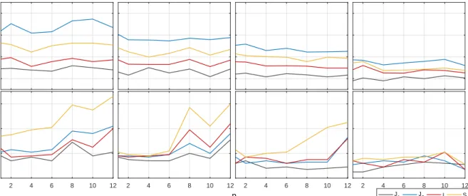
Figure 2: Empirical power of the tests at 5% significance level (AR(1)-GARCH(1,1) model, bootstrap critical values)

0 0.2 0.4 0.6 0.8 1 A₁κ = 0.25 0 0.2 0.4 0.6 0.8 1 0 0.2 0.4 0.6 0.8 1 Rejection frequencies 2 4 6 8 10 12 0 0.2 0.4 0.6 0.8 1 A 1κ = 0.5 2 4 6 8 10 12 A 1κ = 0.75 2 4 6 8 10 12 A 2κ = -2.5 2 4 6 8 10 12 p A 2κ = 2.5 2 4 6 8 10 12 A 3 2 4 6 8 10 12 A 4 T = 250 T = 500 T = 1000 2 4 6 8 10 12 T = 2500 J₁ J₂ I S

Note: Power of the four backtests are displayed as a function ofp. The rows correspond to different sample sizesT, and the columns to the different misspecified alternativesA1-A4. Reported powers are size corrected.

Figure 2 reports the empirical powers (size-corrected) associated with our seven alter-natives. Here, we only present the simulation results associated with the bootstrap critical values. The simulation results obtained with the asymptotic critical values are overall the

same (see Figure 6 in Appendix F). Overall, the tests correctly detect the misspecified alter-natives A1, A2, A3, A4, and we verify that there is a general improvement of powers as the

sample size T increases (from row 1 to row 4), suggesting that these tests are consistent for these alternatives. For instance, with T = 500, and p= 4, the test statistic J1 identifies the

misleading scenario A3 in 49.3% of times, while it reaches 98.1% of times with T = 2500.

Second, the joint test statistics, J1 and J2, generally deliver higher power performances

compared to the intercept and slope test statistics I and S. This finding comes from the definition of the joint null hypotheses that focus on both intercept and slope coefficients and are thus more conservative than the null of the intercept and slope backtests. In details for the two joint tests, we find thatJ1 performs generally better to detectA1 andA4, whileJ2 more

often identifiesA2 and A3, which suggests complementarity between the two joint backtests.

Although the intercept and slope backtests exhibit lower power performances, they provide useful informations on the type of misspecification. In details, the slope backtest performs better in alternatives A1 and A3, while the intercept backtest is superior for alternativeA4.

Thus, A1 and A3 mainly affect the expected value of the slope parameters meaning that

the errors are correlated and proportional to the true quantiles. In contrast, alternative A4

induces distortions in the expected value of the intercept coefficients suggesting that the origin of errors is more global as they are not related to the true quantiles.

Third, we observe that the selection of the number p of risk levels is difficult to link with the rejection frequencies in alternatives A1, A2, A3, since reported powers are slightly

affected by p in general. This finding may be explained by the nature of these alternatives for which the misspecification is relatively uniform along the tail, and does not require many levels. On the contrary, in alternative A4, we conclude that an increase of p is beneficial

for detecting the misleading one-year historical simulation method as power is unequivocally increasing withp, especially whenT is large. This is due to the fact that, for this alternative,

the error made along the tail is more irregular and requires the use of additional levels. Thus, it is helpful to consider,p= 1,2, . . . , pmax, successively, with typicallypmax= 12 as provided

above. This may come in handy for improving the statistical decision.

Finally, we provide a robustness check of the powers with the GARCH(1,1) model (see Figures 8 and 9 in Appendix F). The rejection frequencies are very close to those associated with the AR(1)-GARCH(1,1) model. Consequently, the decision whether to introduce or not a conditional mean in the risk model does not affect the power performances.

5

Empirical application

In this section, we apply our backtests to the daily returns of the S&P500 index. In addition, we provide a method for the adjustment of imperfect forecasts relying on our backtesting framework. In the sequel, we set τ = 0.975 to coincide with the regulatory ES coverage level. The probability levels uj, j = 1,2, . . . , p, are calculated accordingly with Definition

1. In addition, we consider the risk levels suggested by the BCBS, i.e. u1 = 0.975, and

u2 = 0.990, respectively. Finally, for comparison purposes and to provide useful backtesting

recommendations, we consider several values p= 1,2,4,6,8,10,12.

5.1

Data

We consider the daily adjusted closing prices of the S&P500 index over the period January 1, 1997 - December 31, 2012. The in-sample period spans from January 1, 1997 to June 30, 2007, and we use two out-of-sample periods (1) from July 1, 2007 to June 30, 2009, corresponding to the subprime mortgage crisis, and (2) from July 1, 2007 to December 31, 2012, which pools the subprime mortgage crisis and the European sovereign debt crisis, two major episodes of financial instability. We compute the daily log-returns and denote by Lt

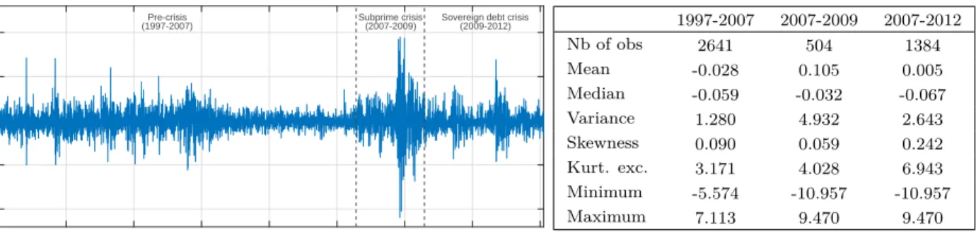
Figure 3: S&P500 daily losses (%), and descriptive statistics 0 500 1000 1500 2000 2500 3000 3500 4000 Observations -10 -5 0 5 10 Ex-post losses

Pre-crisis Subprime crisis Sovereign debt crisis

(1997-2007) (2007-2009) (2009-2012) 1997-2007 2007-2009 2007-2012 Nb of obs 2641 504 1384 Mean -0.028 0.105 0.005 Median -0.059 -0.032 -0.067 Variance 1.280 4.932 2.643 Skewness 0.090 0.059 0.242 Kurt. exc. 3.171 4.028 6.943 Minimum -5.574 -10.957 -10.957 Maximum 7.113 9.470 9.470

Note: The sample covers the period from January 1, 1997 to December 31, 2012. Source: finance.yahoo.comwebsite.

The S&P500 series is depicted in Figure 3 with the three aforementioned sub-periods. The in-sample period (1997-2007) is weakly volatile, while the out-of-sample crisis periods (2007-2009 and 2007-2012) display more severe levels of volatility, with several extreme events. Figure 3 also provides some descriptive statistics. The variance and the average ex-post losses are higher in the out-of-sample periods than in the in-sample period, especially for the period 2007-2009. In addition, the series is right-skewed and has a kurtosis excess.

To predict the ES risk measure, we fit an AR(1)-GARCH(1,1) model with Student inno-vations, as defined in (11), using the S&P500 daily losses of the in-sample period. The ES and VaR forecasts are defined as in Equations (12) and (13), respectively. The set of unknown parameters is estimated by maximum likelihood. We obtain the following coefficient esti-mates nδb₀,δb₁,

b

γ0,γb1,bγ2,vb o

={−0.057,−0.032,0.007,0.060,0.936,9}. As a robustness check, we also fit a GARCH(1,1) model on the same period as defined in the simulation study and for which we obtain the following estimates {γb0,γb1,γb2,vb}={0.007,0.059,0.937,9}.

5.2

Empirical results

We start by evaluating the relevancy of the ES approximation of Definition 1, consisting in averaging several quantiles in the tail of the risk model. To do so, we compare the approximation considering p = 1,2,4,6,8,10,12 quantiles, with what we refer to as "exact ES". The latter corresponds to an ES which is computed via an exact method of calculation.

The technique relies on simulations and is described in Appendix G.

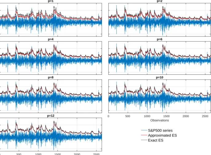
Figure 4: In-sample ES estimates issued from the approximation and the exact calculation method (AR(1)-GARCH(1,1) model)

-5 0 5 p=1 p=2 -5 0 5 p=4 p=6 -5 0 5 Ex-post losses p=8 0 500 1000 1500 2000 2500 Observations p=10 0 500 1000 1500 2000 2500 Observations -5 0 5 p=12 S&P500 series Approximated ES Exact ES

Figure 4 reports the in-sample ES estimates obtained with the approximation and the exact calculation method. Two remarks should be made here. First, the ES forecasts issued from the approximation and the exact method strongly correlate regardless of the value p. The approximation performs very well to capture the ex-post losses information. Second, we observe that the approximation is substantially improved when p slightly increases and coincides almost completely with the exact ES using six (or more) quantiles.

Because the approximation is obtained by combining VaRs, our finding is in accordance with several papers. Gouriéroux and Liu (2012) study the relationship between VaR and ES and show that they are related through their risk levels by some link function. Daníelsson

and Zhou (2016) argue that the two measures of risk are related by a small constant and are conceptually equally informative. This similarity also comes from the structure of the model used to compute the risk measure. For instance, VaR and ES issued by an AR(1)-GARCH(1,1) model have common conditional mean and variance across risk levels implying that these risk measures are closely related (see Equations (12) and (13)). Finally, Figure 10 in Appendix H displays the same results using a GARCH(1,1) model. Removing the condi-tional mean component does not affect the approximation accuracy as the two computation methods match almost perfectly forp≥6. For its ease of implementation and accuracy, the approximation is appealing to compute and evaluate the performance of ES forecasts.

Table 1: p-values of the backtesting tests (AR(1)-GARCH(1,1) model)

p J₁(b) J₂(b) I(b) _S(b) Panel A. 2007-2009 1 0.035 0.051 0.125 0.949 2 0.014 0.041 0.038 0.200 4 0.009 0.040 0.023 0.103 6 0.009 0.038 0.021 0.123 8 0.099 0.049 0.154 0.564 10 0.029 0.061 0.053 0.432 12 0.023 0.052 0.038 0.223 2(regulatory levels) 0.024 0.047 0.053 0.351 Panel B. 2007-2012 1 0.056 0.040 0.176 0.554 2 0.004 0.013 0.014 0.215 4 0.002 0.004 0.003 0.096 6 0.004 0.005 0.009 0.196 8 0.008 0.008 0.041 0.538 10 0.007 0.010 0.021 0.410 12 0.004 0.006 0.008 0.245 2(regulatory levels) 0.006 0.012 0.032 0.448

Note: p-values of the four backtests computed withp= 1,2,4,6,8,10,12 risk levels successively, and the two regulatory levels u1= 0.975,u2= 0.990. Reported p-values are obtained using bootstrap critical values. Panel A gives the results for the period

2007-2009 and Panel B provides results for the period 2007-2012.

Table 1 reports the p-values of the backtests. For a sake of clarity, we only report the p-values obtained with the bootstrap critical values and the results are discussed at 5% significance level. Panel A provides the results over the sample 2007-2009. The test statistic

J1 leads to reject the validity of the ES predictions regardless of the number p of quantiles

observe that the larger p, the smaller the p-value until p= 6, indicating that the rejections are more severe when the number of risk levels increases until an optimal number p. This supports the existence of an upper limit for p which depends on the sample size since T is relatively small (T = 504), and thus, p should not be chosen too large. The test statistic

J2 displays higher p-values in general. The backtest based on a single VaR no longer rejects

the validity of the ES predictions, and the p-value based on the regulatory levels of the BCBS is close to 5%, making the decision rule more unclear for those number of risk levels. Finally, given the p-values of the test statistic I for p = 2,4,6,12, we tend to reject the expected value on the intercept coefficients, and as a result, there is a global bias in the quantile estimates issued by the ES model. On the contrary, the test statisticS leads to the conclusion that the slope parameters are as expected under the null hypothesis, and thus, the magnitude of errors is not related to the true quantiles. Panel B contains the p-values for the period 2007-2012. Overall, we obtain similar results, but the rejections are found more severe in this enlarged sample. Interestingly, the rejections ofJ1are now experienced at a 1%

significance level and even for p >6, as opposed to panel A. This highlights the underlying link between p and T as panel B usesT = 1384 observations enabling a larger number p of quantiles to be used. Table 3 of Appendix H displays the p-values of the backtests when applying a GARCH(1,1) model. The results are similar. Note however, for p = 1, that the p-values are generally higher with the GARCH(1,1) model than for the AR(1)-GARCH(1,1) model. For instance, the p-value of the statistic J1 in panel B equals 0.056 with the

AR(1)-GARCH(1,1) model, while it reaches 0.199 with the AR(1)-GARCH(1,1) model. For that model, additional quantiles are indicated to increase the rejection abilities of the tests.

In sum, we should be cautious in using a single quantile to assess the tail distribution of the risk model. Such procedures may lead market practitioners to select a model that generates mistaken ex-post forecasts. Furthermore, the results issued from the regulatory

guidelines are contrasted. Two risk levels are not always enough to provide a sound conclusion about the correctness of the ES forecasts. We recommend the use of additional risk levels beyond the regulatory coverage level τ = 0.975 to improve the reliability of the decision.

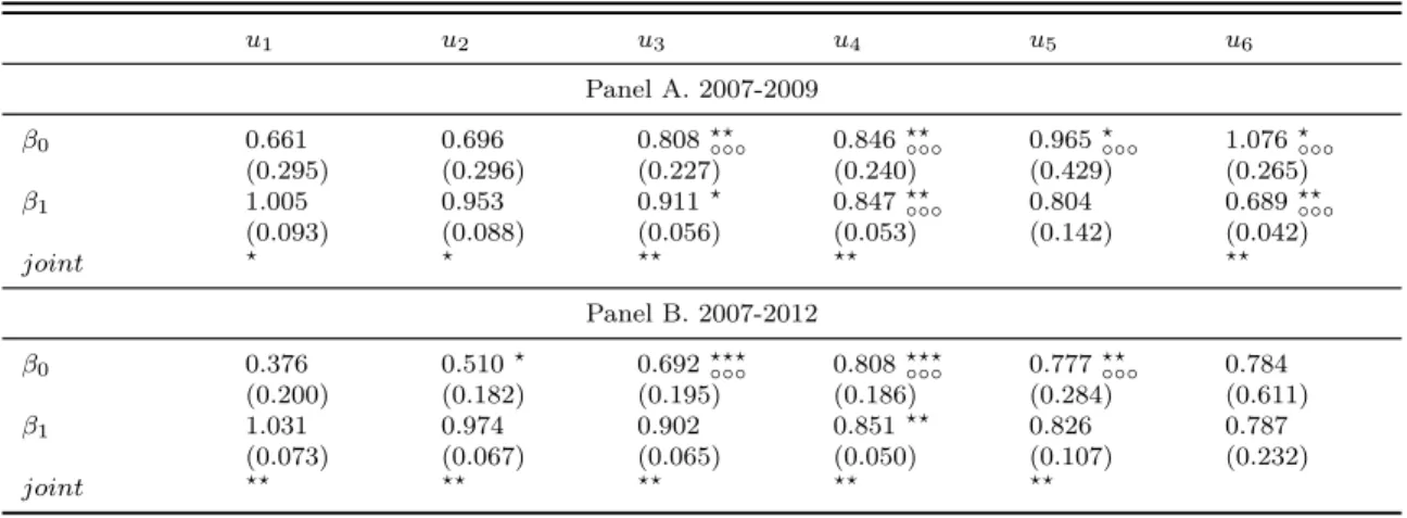
Table 2: QML coefficient estimates (p= 6, AR(1)-GARCH(1,1) model)

u1 u2 u3 u4 u5 u6 Panel A. 2007-2009 β0 0.661 0.696 0.808??◦◦◦ 0.846??◦◦◦ 0.965?◦◦◦ 1.076?◦◦◦ (0.295) (0.296) (0.227) (0.240) (0.429) (0.265) β1 1.005 0.953 0.911? 0.847??◦◦◦ 0.804 0.689??◦◦◦ (0.093) (0.088) (0.056) (0.053) (0.142) (0.042) joint ? ? ?? ?? ?? Panel B. 2007-2012 β0 0.376 0.510? 0.692???◦◦◦ 0.808???◦◦◦ 0.777??◦◦◦ 0.784 (0.200) (0.182) (0.195) (0.186) (0.284) (0.611) β1 1.031 0.974 0.902 0.851?? 0.826 0.787 (0.073) (0.067) (0.065) (0.050) (0.107) (0.232) joint ?? ?? ?? ?? ??

Note: Standard errors are reported in parentheses.?,??, and???indicate statistical significance at the 10%, 5% and 1% level, respectively, and are obtained with the pairs bootstrap algorithm. ◦_,◦◦_{, and}◦◦◦_{, indicate statistical significance at the same}

levels and are obtained with the procedure of Chernozhukov and Fernández-Val (2011). Panel A gives estimation results for the period 2007-2009 and Panel B provides estimation results for the period 2007-2012.

Table 2 displays the coefficient estimates of the multi-quantile regression of Equation (4) for p = 6 risk levels, to help understand the reasons that explain the rejections of the ES forecasts. Panel A and B provide the results for periods 2007-2009 and 2007-2012, respectively. It must be recalled that, if the risk model is correctly specified, the intercept coefficientβ0and the slope coefficientβ1take values zero and one, respectively. We observe in

both panels that the coefficientsβ0are overestimated for all the risk levelsu1, u2, . . . , u6, while

the coefficientβ1 is overestimated for the first levelu1, and it becomes underestimated for all

the remaining risk levelsu2, u3, . . . , u6. The average errors ofβ0andβ1 are respectively equal

to 0.84 and -0.13 in panel A, and 0.66 and -0.10 in panel B, indicating that the magnitude of errors is more important in panel A than in panel B, and that the intercept coefficients are more affected than the slope coefficients. Finally, we observe that the distortion of the regression coefficients with respect to their expected values is more pronounced for the

highest risk levels suggesting that the errors are more severe far in the tail.

Furthermore, we provide in Table 2 one by one inference on the regression parameters with the pairs bootstrap algorithm. The results are depicted with the symbol "∗" and are discussed at a 5% significance level. We observe that the intercept parameters are statistically not equal to zero for the intermediary levels u3 and u4 in panel A, and the additional u5

risk level is also significantly different from zero in panel B. For the slope coefficients, the

u4 and u6 order quantiles are statistically different from one in panel A, and only the level

u4 is misspecified in panel B. In addition, we report joint inference, i.e. looking at both

the intercept and slope coefficients. The results are provided in the row labeled as "joint" (bottom of the panels). Similarly to the previous findings, we find that the intermediary, and highest order quantiles u3, u4 and u6 are misleading in panel A, whereas in panel B, all the

quantiles are misspecified (except for the highest, presumably because the coefficients have large standard errors), meaning that the entire tail distribution is incorrectly estimated.

Next, we propose a variety of robustness checks to our baseline estimation method. Sev-eral alternatives to the QML estimator (White et al., 2008, 2015) and pairs bootstrap (Freed-man, 1981) are available and should be regarded as well. In the sequel, we suggest a number of avenues to be explored. First, we apply the procedure of Chernozhukov and Fernández-Val (2011) based on the extreme value theory (EVT) that allows testing individual restrictions. The results are depicted in Table 2 with the symbol "◦". Overall, we find similar results between EVT and pairs bootstrap. Rejection of the null is mostly experienced at the same levels in panel A and panel B. However, we observe that the procedure of Chernozhukov and Fernández-Val (2011) is generally more powerful than pairs bootstrap at the highest risk levels. For instance, the expected value of the intercept parameters β0(uj) in panel A

is rejected at level 1% for j = 3,4,5,6 with the EVT procedure, while the pairs bootstrap rejects the null at larger levels (5% or 10%). This illustrates the superiority of EVT in

multi-quantile regression models. A robustness check of these results is provided with the GARCH(1,1) model where we overall get the same results (see Table 4 in Appendix H).

Second, we apply the seemingly unrelated regressions (SUR) estimation method for quan-tile models of Jun and Pinkse (2009). The procedure is designed to improve estimation efficiency in presence of correlated generalized errors. In our framework, the risk levels uj,

j = 1,2, . . . , p, are closed to each other, and the correlation may be important between different quantiles. Consequently, the QML estimation method may loose a lot in accuracy. In the sequel, we compute the backtesting tests based on the quantile regression parameter estimates of Jun and Pinkse (2009). Table 5 of Appendix H reports the corresponding boot-strap p-values. The test statistics J1, J2, I, lead to reject the validity of the ES estimates

while the statistic S does not. These findings are similar with those of the QML estimates (see Table 1). Our conclusions are not affected by the choice of the estimation method (SUR vs. QML estimation). Table 6 of Appendix H displays the coefficient estimates computed with the SUR-estimation procedure. We observe that the SUR estimates βb₀ and βb₁ are

close to the QML ones, explaining why our conclusions of our backtests are robust. Second, we note that the asymptotic standard errors of the SUR-estimator are not always close to those of the QML estimation method. The largest differences occur at risk levels u5 for

the slope parameter (in panels A and B) and u6 for both parameters (in panel B), where

standard errors are typically more than twice lower than those of the QML estimator. This confirms the efficiency improvement achieved by the SUR-estimator. Our conclusions with the GARCH(1,1) model are the same (see Tables 7 and 8 in Appendix H).

5.3

Adjusted ES forecasts

In what follows, we exploit our testing strategy to provide adjusted ES forecasts. Our routine is designed to take into account both misspecification and estimation uncertainty,

without having to change the misspecified risk model. Furthermore, the procedure may serve to identify whether the model overestimates, or underestimates the true unknown ES, by comparing the initial forecast with its adjusted counterpart, which appears useful in a risk management and regulatory viewpoint.

The correction of imperfect risk forecasts is not a novel concept in the financial literature. Gouriéroux and Zakoïan (2013) propose to adjust the VaR forecasts affected by estimation uncertainty. Similarly, Boucher et al. (2014) adjust imperfect VaR forecasts based on back-testing frameworks, and recently Lazar and Zhang (2019) apply the same strategy to adjust imperfect ES forecasts. The method typically consists in modifying the coverage level τ of the risk measure so as to meet the null hypothesis of valid risk forecasts. The originality of our technique stems from the fact that we employ a regression-based framework to cor-rect the ex-ante forecasts, while available techniques are generally based on the concept of violation. This allows us to directly adjust the risk forecasts by application of a regression model, without having to rescale the coverage level τ.

For ease of notation, we assume the parameters of the multi-quantile regression to be known. Formally, the adjusted VaR forecast at leveluj, and timet, is defined as the ex-ante

prediction of the multi-quantile regression model, namelyQLt(uj; Ωt−1). In view of Equation

(5), the initial imperfect VaR forecast is subsequently weighted by the regression parameters

β0(uj) and β1(uj), which provides an adjustment corresponding to the global bias caused

by misspecification and estimation uncertainty. The adjusted ES forecast at coverage level

τ and time t is derived from the ES approximation as follows:

ES_t∗(τ) = 1 p p X j=1 QLt(uj; Ωt−1).

The adjusted ES forecasts are robust to model risk, as they meet the desirable properties on the regression coefficients. Indeed, if we compute the backtesting procedure with the

sequence{QLt(uj; Ωt−1)} p

j=1instead of the initial misleading{V aRt(uj)}pj=1, the parameters

would exactly coincide with the expected values under the null hypothesis, i.e. β0(uj) = 0,

and β1(uj) = 1, for the risk levelsu1, u2, . . . , up.

Figure 5: ES forecasts and adjusted ES forecasts over the period 2007-2009 (AR(1)-GARCH(1,1) model) 2 4 6 8 10 12 p=1 p=2 2 4 6 8 10 12 p=4 p=6 2 4 6 8 10 12 ES forecasts p=8 0 50 100 150 200 250 300 350 400 450 500 Observations p=10 0 50 100 150 200 250 300 350 400 450 500 Observations 2 4 6 8 10 12 p=12 ES forecasts Adjusted ES forecasts

Figure 5 reports the ES predictions and adjusted ES predictions for the period 2007-2009. The forecasts are built using the approximation withp= 1,2,4,6,8,10,12. We observe that the AR(1)-GARCH(1,1) model generally provides underestimated forecasts compared to the adjusted predictions. The underestimation is more pronounced for the smallest predictions, the error being more severe when the risk forecasts are originally small. Thus, our procedure serves at identifying whether the model generates overestimates or underestimates, the latter case being more worrisome in a financial stability perspective. Finally, the ES forecasts are

slightly overestimated when the variance of the series is larger, suggesting that the risk model may overestimate the true volatility in turbulent financial times. This is due to the volatility persistence in the GARCH component. Our findings are robust to (1) the use of a simple GARCH(1,1) model, (2) the use of the two BCBS regulatory levels, and (3) the extended period 2007-2012 (see Figures 11, 12, 13, and 14 in Appendix H).

6

Conclusion

The financial crisis of 2007-2008 and its aftermath has led to a reassessment of risk-management practices and financial market regulation through the Basel III accords (BCBS, 2010). Among the number of fundamental reforms for the market risk, the BCBS has adopted ES in place of VaR as the new standard for risk management. One of the major obstacle to its implementation was the deficit of simple tools for the evaluation of its forecasts. This ar-ticle introduces four easy-to-use regression-based backtests of ES. Our econometric approach consists in regressing the ex-post losses on the VaRs forecasts in a multi-quantile regression model, and then, testing the resulting parameter estimates using Wald-type inference.

Several simulation studies are provided. We find that the use of asymptotic critical values may lead to important size distortions if the sample size is not large enough. We propose a pairs bootstrap algorithm to correct these small-sample biases (Freedman, 1981) and show that our regression-based tests are reasonably sized within this bootstrap framework. We consider several misleading alternatives in line with the existing literature on risk assessment (Gaglianone et al., 2011; Du and Escanciano, 2017; Bayer and Dimitriadis, 2019; Kratz et al., 2018, etc.). Our methodology detect misspecifications in all considered simulation experiments. In particular, they identify the most frequent inaccuracies in risk modeling, namely mean, variance, tail, and dynamic misspecifications.