Bayesian Learning of Impacts of Self-Exciting Jumps
in Returns and Volatility
Andras Fulop, Junye Li, and Jun Yu
January 2012
Bayesian Learning of Impacts of Self-Exciting Jumps
in Returns and Volatility
∗Andras Fulop, Junye Li, and Jun Yu
First Version: May 2011; This Version: December 2011
Abstract
The paper proposes a new class of continuous-time asset pricing models where negative jumps play a crucial role. Whenever there is a negative jump in asset re-turns, it is simultaneously passed on to diffusion variance and the jump intensity, generating self-exciting co-jumps of prices and volatility and jump clustering. To properly deal with parameter uncertainty and in-sample over-fitting, a Bayesian learning approach combined with an efficient particle filter is employed. It not only allows for comparison of both nested and non-nested models, but also gener-ates all quantities necessary for sequential model analysis. Empirical investigation using S&P 500 index returns shows that volatility jumps at the same time as neg-ative jumps in asset returns mainly through jumps in diffusion volatility. We find substantial evidence for jump clustering, in particular, after the recent financial crisis in 2008, even though parameters driving dynamics of the jump intensity remain difficult to identify.
KEY WORDS: Self-Excitation, Volatility Jump, Jump Clustering, Extreme Events, Parameter Learning, Particle Filters, Sequential Bayes Factor, Risk Man-agement
JEL Classification: C11, C13, C32, G12
∗Andras Fulop, Finance Department, ESSEC Business School, Paris-Singapore, Cergy-Pontoise
Cedex, France 95021. Junye Li, Finance Department, ESSEC Business School, Paris-Singapore, 100 Victoria Street, Singapore 188064. Jun Yu, Sim Kee Boon Institute for Financial Economics, School of Economics, and Lee Kong Chian School of Business, Singapore Management University, 90 Stamford Road, Singapore 178903. We thank the Risk Management Institute at National University of Singapore for providing us the computing facility. Fulop and Li’s research is funded by ESSEC Research Center.
1
Introduction
The financial meltdown of 2008 and the recent European debt crisis in 2011 raise
ques-tions about how likely extreme events are and how extreme events can be modeled
as they have already impacted financial markets worldwide and have had far-reaching
consequences for the world economy. Understanding dynamics of extreme events thus
becomes crucial to many financial decision makings, including investment decision,
hedging, policy reaction and rating. An important class of models is the
continuous-time diffusions (Hull and White, 1986; Heston, 1993), which can effectively capture
stochastic volatility and volatility clustering. However, empirical explorations have
found that extreme events in asset prices are very unlikely to happen under standard
diffusion models and a jump component is needed to capture discontinuous movements
in asset prices. Both parametric and nonparametric studies provide strong and
con-vincing evidence on significance of jumps in asset returns1.
However, only stochastic volatility and jumps in asset returns may not capture
the real dynamics of asset prices and therefore cannot generate enough probability of
extreme events. It has been recognized that a big jump, in particular a big negative
jump in asset prices, tends to be associated with an abrupt move in asset volatility,
i.e., co-jumps of prices and volatility. Furthermore, market turmoils seem to tell that
an extreme movement in markets tends to be followed by another extreme movement,
resulting in jump clustering. To document these facts, Table 1 reports the S&P 500
index returns and the corresponding standard deviations computed using the previous
22-day returns during the four turbulent periods, covering the Black Monday in 1987,
the crash of the Internet Bubble in 2002, the bankruptcy of Lehman Brothers during
the global financial crisis in 2008, and the European debt crisis in 2011. In all turbulent
periods, extreme price movements are accompanied by high volatility and both extreme
events and volatility are cluttered.
1Parametric studies include Bates (1996, 2000), Bakshi, Cao, and Chen (1997), Pan (2003), Eraker,
Johannes and Polosn (2003), Eraker (2004), among others, whereas nonparametric works include Barndorff-Nielson and Shephard (2007), A¨ıt-Sahalia and Jacod (2009, 2011), Cont and Mancini (2008), and Lee and Hannig (2010)
— Table 1 around here —
Obviously, diffusion-based multi-factor volatility models are not good enough for
capturing co-jumps of prices and volatility and jump clustering as there is no
mech-anism to trigger extreme movements in asset returns and volatility during a turmoil.
Not surprisingly, Bates (2000) and Chernov et al. (2003) have found that the two-factor
volatility model does not offer substantial improvements over the single-factor volatility
model. In the literature, two strands, which have pursued to accommodate co-jumps
of prices and volatility and jump clustering, co-exist. One strand uses synchronized
Poisson process to model asset returns and diffusion volatility (Duffie, Pan, and
Sin-gleton, 2000; Eraker, Johannes, and Polson, 2003; Eraker, 2004). In this framework,
a jump arrives in returns and diffusion volatility that not only moves price but also
pushes up diffusion volatility. Since the process for diffusion volatility is persistent,
another large volatility value is expected in the next period. Consequently, another
extreme movement in asset price is highly likely to be followed, even if there is no jump
arrival. Another strand proposes a mechanism whereby jumps in asset returns feedback
to the jump intensity, leading to self-excitation (A¨ıt-Sahalia, Cacho-Diaz, and Laeven,
2010; Carr and Wu, 2010). Here, large jumps in asset returns increase the likelihood of
extreme events in future asset returns and generate aggregate volatility jumps through
the jump intensity.
While both approaches can generate co-jumps of prices and volatility and a
correla-tion structure in extreme price movements, the implicacorrela-tions of them are different. First,
the propagating mechanism of extreme events is different. In particular, the correlation
in extreme events is driven by the correlation in the high volatility regime in the former
approach but by the correlation in the intensity in the latter. Second, the amount of
conditional kurtosis generated by the two approaches is likely to be different. As the
sampling interval gets smaller, it is expected that the impact of diffusion volatility on
the kurtosis is smaller than that of jumps. Thus the amount of short-term tail risk
after a market crash is likely to differ in the two cases. These differences inevitably
is important to empirically examine the relative importance of these two alternative
mechanisms.
In the present paper, we propose a new class of continuous-time asset pricing
mod-els where both channmod-els of co-jumps of prices and volatility and jump clustering are
allowed. In our specification, negative jumps play crucial roles. Whenever there is
a negative jump in asset returns, it is simultaneously passed on to diffusion variance
and the jump intensity. Therefore, the likelihood of the future extreme events can be
enhanced through jumps in diffusion volatility or jumps in the jump intensity or both.
The importance of negative jumps can be motivated from empirical observations in
Table 1 where in all cases turmoils start with negative jumps. It is also consistent
with our understanding of financial markets where investors are more sensitive to
ex-treme downside risk. Our model has closed-form conditional expectation of volatility
components, making it easy to use in volatility forecasting and risk management.
The new model contains multiple dynamic unobserved factors including diffusion
volatility, the jump intensity, and (negative and positive) jumps. Since a richer model
framework is adopted here, we are naturally concerned about parameter uncertainty
and in-sample over-fitting inherent in batch estimation. To deal with these issues, we
introduce a Bayesian learning approach for the proposed model. In practice, sequential
estimation of both parameters and latent factors is much more relevant than batch
estimation as we cannot obtain future information and need to update our belief
when-ever new observations arrive. First, to filter the unobserved states and estimate the
likelihood for a given set of model parameters, we develop an efficient hybrid particle
filter. It efficiently disentangles the diffusion component and the positive and negative
jumps. The algorithm performs much better than the conventional bootstrap sampler
for outliers that are an integral part of the financial data and of our model. Second,
we turn to a sequential Bayesian procedure to conduct joint inference over the dynamic
states and fixed parameters. In particular, we employ the marginalized resample-move
effort from users2. The essence of the approach is to approximately marginalize out
the hidden states by running a particle filter for fixed parameter sets. Then a recursive
resample-move algorithm is used on the marginalized system. The algorithm provides
marginal likelihoods of individual observations that are crucial for sequential model
analysis with respect to information accumulation over time. It is important to point
out that the simulated samples obtained at any time only depend on past data so the
approach is free from hindsight bias.
We use S&P 500 index returns ranging from January 2, 1980 to October 30, 2011
(in total, 8,033 observations) to empirically investigate our self-exciting models. This
dataset is long enough and contains typical market behaviors: the 87’s market crash, the
98’s Asian financial crisis, the 02’s dot-com bubble burst, the 08’s global financial crisis,
the 11’s European debt crisis, and calm periods in between. We find that both sources of
co-jumps in volatility and returns help explain our dataset. The evidence for the channel
through diffusion volatility is robust ever since the 1987 market crash. The parameter
driving the feedback from negative return jumps to diffusion volatility is well identified
and less than one. In contrast, the self-exciting jump intensity becomes important at the
onset of the 08’s global financial crisis. The out-of-sample model diagnostics suggest
that the data call for co-jumps in returns and jump intensities, but the parameters
driving the intensity dynamics remain hard to identify. The substantial uncertainty
about the jump dynamics is mirrored in large uncertainty about the magnitude of
jump intensities during the recent financial crisis.
Our results have important implications for risk management. As diffusion volatility
jump is a necessary component in modeling the stock market index and volatility
co-jumps at the same time as negative co-jumps in asset returns, traditional hedging strategies
such as only using the underlying assets and/or using both underlying and derivatives
are no longer workable. We show that different models have different VaR requirements,
2There has already been progress towards tackling parameter learning in general state-space models.
See Liu and West (2001), Gilks and Berzouini (2001), Storvik (2002), Flury and Shephard (2009), and Carvalho et al. (2010). For discussion of these methods, see Fulop and Li (2010). For a similar and concurrent contribution, see Chopin et al. (2011).
especially at financial crises. Models with diffusion volatility jumps are capable of
generating high enough values of VaR when extreme events happen. Furthermore,
the big uncertainty in the jump intensity may lead to important risk management
implications in the form of substantially higher tail risk measures.
The paper makes three separate contributions to the literature. First, a new class
of continuous-time asset pricing models is proposed. It provides a nice framework
to investigate where volatility jump is from and how it interacts with jumps in asset
returns. Second, a generic econometric approach is developed that allows us to perform
joint sequential inference over the states and the parameters with respect to information
accumulation over time. Third, we provide new insights to extreme price movements
and co-jumps of prices and volatility.
Our work is related to previous studies. Jacod and Todorov (2010) and Bandi and
Reno (2011) find that asset returns and their volatility jump together. Their results are
based on high frequency data that become available only after 1990s. The use of daily
data allows us to go much further back into the history. One advantage of using a longer
time span is that we can have more jumps and hence potentially more episodes of jump
clustering. Focusing completely on the volatility dynamics, Wu (2011) and Todorov and
Tauchen (2011) show that volatility does jump. Our results are in accord with them
but we go further and allow two different channels through diffusion volatility and the
jump intensity. This also differentiates us from existing papers where either only the
diffusion channel is present (Eraker, Johannes, and Polson, 2003; Eraker, 2004) or only
the jump intensity is affected by return jumps (A¨ıt-Sahalia, Cacho-Diaz, and Laeven,
2010; Carr and Wu, 2010). We find that the diffusion channel is more important and
remains significant even when the jump channel is allowed. As of the jump channel,
our results are weaker than in A¨ıt-Sahalia, Cacho-Diaz, and Laeven (2010) and Carr
and Wu (2010). This may be either due to the differences in the samples, or to the fact
that our specification is more general.
The rest of the paper is organized as follows. Section 2 builds the self-exciting
introduces our Bayesian learning algorithm. Section 4 presents empirical results and
discuss their implications using S&P 500 index returns. Finally, section 5 concludes
the paper. Detailed algorithms of the particle filter and Bayesian learning are given in
Appendices.
2
Self-Exciting Asset Pricing Models
Under a probability space (Ω,F, P) and the complete filtration{Ft}t≥0, the asset price
St has the following dynamics
lnSt/S0 = ∫ t 0 µsds+ ( WT1,t −kW(1)T1,t ) + ( JT2,t−kJ(1)T2,t ) , (1)
whereµt is the instantaneous mean,W is a Brownian motion, J is a jump component,
andkW(1) andkJ(1) are convexity adjustments for the Brownian motion and the jump
process and can be computed from their cumulant exponents: k(u) ≡ 1tln
(
E[euLt] )
,
where Lt is eitherWt orJt.
The dynamics (1) indicates two distinct types of shocks to asset returns: small
continuous shocks, captured by a Brownian motion, and large discontinuous shocks,
modeled in this paper by the Variance Gamma process of Madan, Carr, and Chang
(1998), a stochastic process in the class of infinite activity L´evy processes. The jump
component is important for generating the return non-normality and capturing extreme
events. The empirical study by Li, Wells, and Yu (2008) shows that the infinite activity
L´evy models outperform the affine Poisson jump models. Furthermore, the recent
nonparametric works by A¨ıt-Sahalia and Jacod (2009, 2011), Cont and Mancini (2008),
and Lee and Hannig (2010) provide strong evidence on infinite activity jumps in asset
returns.
The Variance Gamma process can be constructed through subordinating a Brownian
motion with drift using an independent subordinator
where ˜Wtis a standard Brownian motion, andStis a subordinator that has the Gamma
process St = Γ(t; 1, v) with unit mean rate and variance rate v. Alternatively, it can
be decomposed into the upside component,Jt+, and the downside component,Jt−, such
that
Jt = Jt++Jt−,
= Γu(t;µu, vu)−Γd(t;µd, vd), (3)
where Γu is a Gamma process with mean rate µu and variance ratevu, Γd is a Gamma
process with mean rate µd and variance rate vd, and
µu = 1 2 (√ ω2+ 2η2/v+ω ) , vu =µ2uv, (4) µd = 1 2 (√ ω2+ 2η2/v−ω ) , vd=µ2dv. (5)
Ti,t defines a stochastic business time (Clark, 1973; Carr et al., 2003; Carr and Wu,
2004), which captures the randomness of the diffusion variance (i= 1) or of the jump
intensity (i= 2) over a time interval [0, t]
Ti,t =
∫ t 0
Vi,s−ds,
which is finite almost surely. Vi,t, which should be nonnegative, is the instantaneous
variance rate (i = 1) or the jump arrival rate (i = 2), both of them reflecting the
intensity of economic activity and information flow. Stochastic volatility or stochastic
jump intensity is generated by replacing calendar time t with business time Ti,t. The
time-changed jump component has the decomposition of JT2,t = J
+ T2,t +J
−
T2,t and its
convexity adjustment term iskJ(1)T2,t =
(
k+J(1) +kJ−(1)
) T2,t.
following stochastic differential equations
dV1,t = κ1(θ1−V1,t)dt+σ11
√
V1,tdZt−σ12dJT−2,t, (6) dV2,t = κ2(θ2−V2,t)dt−σ2dJT−2,t, (7)
Equation (6) captures stochastic variance of the continuous shocks, whereZ is a
stan-dard Brownian motion and is allowed to be correlated toW with a correlation parameter
ρin order to accommodate the diffusion leverage effect. Diffusion variance also depends
on the negative jumpsJ−, indicating that there will be an abrupt increase in V1,t once
there is a negative jump in asset price. If κ1 is positive and small, Equation (6)
sug-gests a persistent autoregressive structure inV1,t. An abrupt increase inV1,t would then
imply that the future diffusion variance tends to be high and decays exponentially at
the speedκ1. Equation (7) models the stochastic intensity of jumps. Whenκ2 >0, it is
a mean-reverting pure jump process. The specification implies that the jump intensity
relies only on the negative jumps in asset returns.
The conditional expectation of the jump intensity (7) can be found as follows3
E[V2,t|V2,0] = κ2θ2 κ2−σ2µd ( 1−e−(κ2−σ2µd)t ) +e−(κ2−σ2µd)tV 2,0, (8)
from which its long-run mean can be obtained by lettingt →+∞,
¯
V2 =
κ2θ2
κ2−σ2µd
. (9)
Solutions (8) and (9) indicate that the conditional expectation of the jump intensity is
a weighted average between the current intensity,V2,0, and its long-run mean, ¯V2. Using
(8) and (9), the conditional expectation of diffusion variance (6) can also be analytically
3Definef(t) =eκ2tE[V
2,t|V2,0]. f(t) can be analytically found by solving the ODE
f′(t) =σ2µdf(t) +κ2θ2eκ2t,
found E[V1,t|V1,0] = e−κ1tV1,0+θ1 ( 1−e−κ1t ) +σ12µd [1−e−κ1t κ1 ¯ V2 +e −(κ2−σ2µd)t−e−κ1t κ2−σ2µd−κ1 ( ¯ V2−V2,0 )] , (10)
and its long-run mean is given by
¯
V1 =θ1+
σ12
κ1
µdV¯2. (11)
The conditional expectation of diffusion variance composes of two parts, one arising
from the square-root diffusion part (the first two terms on the right-hand side in (10))
and the other from negative return jumps (the last term on the right-hand side in
(10)). If the jump intensity is constant, the contribution of jumps to the conditional
diffusion variance becomes constant over time. In what follows, we normalize θ2 to be
one in order to alleviate the identification problem because the jump component, J,
has non-unit variance.
Dependence of diffusion variance and the jump intensity only on negative jumps in
asset returns is a consistent observation obtained from Table 1 where turmoils always
start with negative jumps. It is also consistent with the well documented empirical
reg-ularity in financial markets that react more strongly to bad macroeconomic surprises
than to good surprises (Andersen et al., 2007). This is because the stability and
sus-tainability of future payoffs of an investment are largely determined by extreme changes
in economic conditions, and investors are more sensitive to the downside movements in
the economy.
The above model (hereafterSE-M1) indicates that time-varying aggregate volatility
is contributed by two sources: one arises from time-varying diffusion volatility and
the other from the time-varying jump intensity. Whenever there is a negative jump
in asset return, diffusion volatility and the jump intensity move up significantly and
captured through two channels: (i) a negative jump in asset return pushes up the jump
intensity, which in turn triggers more jumps in future asset returns; (ii) a negative jump
in asset return makes diffusion volatility jump, and this high diffusion volatility tends to
entertain big movements in future asset returns. In contrast, existing literature allows
only one of these channels at a time. In particular, Eraker, Johannes, and Polson (2003)
and Eraker (2004) allow co-movement of return jumps and diffusion volatility through
a synchronized Poisson process, while A¨ıt-Sahalia, Cacho-Diaz, and Laeven (2010) and
Carr and Wu (2010) link only the jump intensity to jumps in asset returns.
The central questions we are concerned about in the present paper are the dynamic
structure of extreme movements and how asset return jumps affect total volatility. In
order to explore these issues, we also investigate the following nested models: (i)
SE-M2: the self-exciting model where diffusion volatility does not jump, and the total
volatility jump and the the jump clustering are from the time-varying jump intensity;
(ii) SE-M3: the model where the jump intensity is constant, and the total volatility
jump and the self-exciting effect are only from the diffusion volatility process; and (iii)
SE-M4: no volatility jumps and no self-exciting effects. Obviously, the SE-M4 model
is nested by the SE-M2 model and the SE-M3 model. However, the SE-M2 model and
the SE-M3 model do not nest each other.
3
Econometric Methodology
In this section, we present our Bayesian learning method. Section 3.1 develops an
efficient hybrid particle filter, which provides us more accurate likelihood estimate and
separates the diffusion component, positive jumps and negative jumps. Section 3.2
briefly presents the parameter learning algorithm for model estimation.
3.1
An Efficient Hybrid Particle filter
Our model can be cast into a state-space model framework. After discretizing the return
equation lnSt= lnSt−τ+ ( µ− 1 2V1,t−τ −k(1)V2,t−τ ) τ +√τ V1,t−τwt+Ju,t +Jd,t, (12)
where wt is a standard normal noise, and Ju,t and Jd,t are the upside and downside
jumps.
We take the diffusion varianceV1,t, the jump intensityV2,t, and the upside/downside
jumps Ju,t/Jd,t as the hidden states. Diffusion variance and the jump intensity follow
(6) and (7), and the upside/downside jumps are gammas. After discretizing, we have
the state equations as follows
V1,t = κ1θ1τ+ (1−κ1τ)V1,t−τ+σ11 √ τ V1,t−τzt−σ12Jd,t, (13) V2,t = κ2θ2τ+ (1−κ2τ)V2,t−τ−σ2Jd,t, (14) Ju,t = Γ(τ V2,t−τ;µu, vu), (15) Jd,t = −Γ(τ V2,t−τ;µd, vd), (16)
whereztis a standard normal noise, which is correlated towtin (12) with the correlation
parameter ρ.
For a given set of model parameters, Θ, filtering is a process of finding the
pos-terior distribution of the hidden states based on the past and current observations,
p(xt|y1:t,Θ), where xt={V1,t, V2,t, Ju,t, Jd,t}, and y1:t ={lnSs}ts=1. Because this
poste-rior distribution in our model does not have analytical form, we turn to particle filters
to approximate it. Particle filters are simulation-based recursive algorithms where the
posterior distribution is represented by a number of particles drawn from a proposal
density ˆ p(xt|y1:t,Θ) = M ∑ i=1 ˜ w(ti)δ ( xt−x (i) t ) , (17)
where ˜w(ti) = ωt(i)/∑Mj=1ωt(j) with ωt and ˜wt being the importance weight and the
the Dirac delta function.
Particle filters provide an estimate of the likelihood of the observations
ˆ p(y1:t|Θ) = t ∏ l=1 ˆ p(yl|y1:l−1,Θ), (18) where ˆ p(yl|y1:l−1,Θ) = 1 M M ∑ i=1 wl(i). (19)
Importantly, the approximated likelihood (18) is unbiased: E[ˆp(y1:t|Θ)] =p(y1:t|Θ) (Del
Moral, 2004), where the expectation is taken with respect to all random quantities used
in particle filters.
The most commonly used particle filter is the bootstrap filter of Gordon, Salmond,
and Smith (1993), which simply takes the state transition density as the proposal
density. However, the bootstrap filter is known to perform poorly when the observation
is informative on the hidden states. Our model has this feature because when we observe
a large move in asset price, the jump can be largely pinned down by the observed return.
On the other hand, when the return is small, it is almost due to the diffusion component
and contains litter information on the jump. Hence, to provide an efficient sampler, we
use an equally weighted two-component mixture as the proposal on the jump: the first
component is a normal draw, equivalent to sampling from the transition density of the
diffusion component, and the second component involves drawing from the transition
law of the jump. We need this second component to stabilize the importance weights
for small observed returns. Otherwise, we would compute the ratio of a normal and
a gamma density in the importance weights which is unstable around zero. When
the return is positive, we use this mixture as the proposal for the positive jump and
the transition density for the negative jump, and vice-versa. See Appendix A for the
3.2
A Parameter Learning Algorithm
While particle filters make state filtering relatively straightforward, parameter learning,
i.e., drawing from p(Θ|y1:t) sequentially, remains a difficult task. Simply including the
static parameters in the state space and applying a particle filter overp(Θ, xt|y1:t) does
not result in a successful solution due to the time-invariance and stochastic singularity
of the static parameters that quickly leads to particle depletion. In what follows, we use
a generic solution to the parameter learning problem proposed by Fulop and Li (2010).
The key to this algorithm is that particle filters provide an unbiased estimate of the true
likelihood, so that we can run a recursive algorithm over the fixed parameters using the
sequence of estimated densities, ˆp(Θ|y1:t)∝
∏t
l=1pˆ(yl|y1:l−1,Θ)p(Θ), fort= 1,2, . . . , T.
Define an auxiliary state space by including all the random quantities produced by
the particle filtering algorithm. In particular, denote the random quantities produced
by the particle filter in steplbyul ={x (i) l , ξ
(i)
l ;i= 1, . . . , M}. Then at timet, the filter
will only depend on the population of the state particles in step t−1, so we can write
ψ(u1:t|y1:t,Θ) = t
∏
l=1
ψ(ul|ul−1, yl,Θ), (20)
whereψ(u1:t|y1:t,Θ) is the density of all the random variables produced by the particle
filter up to t. Furthermore, the predictive likelihood of the new observations can be
written as
ˆ
p(yt|y1:t−1,Θ) ≡pˆ(yt|ut, ut−1,Θ). (21)
We then construct an auxiliary density, which has the form
˜ p(Θ, u1:t|y1:t)∝p(Θ) t ∏ l=1 ˆ p(yl|ul, ul−1,Θ)ψ(ul|ul−1, yl,Θ). (22)
The unbiasedness property in likelihood approximation means that the original target,
p(Θ|y1:t), is the marginal distribution of the auxiliary density. If we can sequentially
draw from the auxiliary density, we automatically obtain samples from the original
Assume that we have a set of weighted samples that represent the target distribution, ˜ p(Θ, u1:t−1|y1:t−1), at timet−1: {( Θ(n), u(n) t−1,pˆ(y1:t−1|Θ)(n) ) , s(tn−)1;n= 1, . . . , N } , where
st−1 denotes the sample weight. Notice that for each n, the relevant part of u (n) t−1
are M particles after resampling representing the hidden states {x(ti,n);i = 1, . . . , M}. Therefore, in total we have to maintain M ×N particles of the hidden states. The following recursive relationship holds between the target distributions at t−1 and t,
˜
p(Θ, u1:t|y1:t)∝pˆ(yt|ut, ut−1,Θ)ψ(ut|ut−1, yt,Θ)˜p(Θ, u1:t−1|y1:t−1), (23)
from which we can arrive to a set of samples representing the target distribution,
˜
p(Θ, u1:t|y1:t), at time t through the marginalized resample-move approach developed
by Fulop and Li (2010). See Appendix B for an outline of the algorithm.
The marginalized resample-move approach has a natural byproduct of the marginal
likelihood of the new observation
p(yt|y1:t−1) ≡
∫
p(yt|y1:t−1,Θ)p(Θ|y1:t−1)dΘ, (24)
from which a sequential Bayes factor can be constructed for sequential model
compari-son. For any models M1 and M2, the Bayes factor at time t has the following recursive
formula BFt≡ p(y1:t|M1) p(y1:t|M2) = p(yt|y1:t−1, M1) p(yt|y1:t−1, M2) BFt−1. (25)
Our particle learning algorithm naturally has the marginal likelihood estimate (29),
which can be used in (25) for model assessment and monitoring over time.
4
Empirical Results
In this section, we present estimation results and discuss their empirical implications.
Models are estimated using the Bayesian learning approach discussed in Section 3. In
of parameter particles to be 2,000. The thresholds N1 and N2 are equal to 1,000.
These tuning-parameters are chosen such that the acceptance rate at the move step is
relatively high and the computational cost is reasonable. Section 4.1 presents the data
used for model estimation, and Section 4.2 discusses the empirical results.
4.1
Data
The data used to estimate the models are the S&P 500 stock index ranging from January
2, 1980 to October 30, 2011 in daily frequency, in total 8,033 observations. This dataset
contains typical financial market behaviors: the recent European debt crisis, the global
financial crisis in the late 2008, the market crash on October 19, 1987 (-22.9%), the
volatile market and relatively tranquil periods. Table 2 presents descriptive statistics
of index returns. The annualized mean of index returns in this period is around 7.8%
and the annualized historical volatility is about 18.4%. A striking feature of the data
is high non-normality of the return distribution with the skewness of -1.19 and the
kurtosis of 29.7. The Jarque-Bera test easily rejects the null hypothesis of normality
of returns with a very small p-value (less than 0.001). The index returns display very
weak autocorrelation. The first autocorelation is about -0.03, while the sixth one is as
small as 0.008.
— Table 2 around here —
Figure 1 plots S&P 500 index returns and standard deviations computed from the
previous 22-day returns at each time. The companion of abrupt moves in volatility
to extreme events in returns is very clear, and turbulent periods tend to be realized
through many consecutive large up and down return moves. What is hard to gauge is
the extent to which these are due to high diffusion volatility or persistent fat tails. The
model estimates that follow will shed more lights on this issue.
4.2
Estimation and Empirical Implications
A. Model Monitoring and Diagnostics
In a Bayesian context, model comparison can be made by the Bayes factor, defined
as the ratio of marginal likelihoods of models4. Table 3 presents the overall Bayes
factors (in log) for all models investigated using all available data. We find that the
SE-M1 model and the SE-M3 model, both of which allow negative return jumps to
affect diffusion volatility, outperforms the SE-M2 model and the SE-M4 model that
exclude this channel. For example, the log Bayes factors between the SE-M1 model
and the SE-M2/SE-M4 models are about 18.4 and 19.2, respectively, and the log Bayes
factors between the SE-M3 model and the SE-M2/SE-M4 models are about 14.3 and
15.1, respectively. Thus, there is considerable evidence in the data for negative return
jumps affecting diffusion volatility and co-jumps of returns and volatility. Furthermore,
there seems to be evidence for return jumps affecting the jump intensity. Comparing
the SE-M1 model where both self-exciting channels are allowed to the SE-M3 model
where only diffusion volatility is influenced by return jumps, the former is preferred
with a log Bayes factor of 4.11.
— Table 3 around here —
The above batch comparison does not tell us how market information accumulates
and how different models perform over time. Does one model outperform the other one
at a certain state of economy, but underperforms it at another state of economy? Our
Bayesian learning approach has a recursive nature and produces the individual marginal
likelihood of each observation over time. One can then construct the sequential Bayes
factors and use them for real-time model monitoring and analysis.
Figure 2 presents the sequential Bayes factors (in log) that gives us a richer picture
on model performance over time. We notice from the upper panels that in the beginning
when market information is little, both the SE-M1 model and the SE-M3 model, which
4In Bayesian statistics, for two modelsM
1andM2, if the value of the log Bayes factor ofM1toM2
is between 0 and 1.09,M1is barely worth mentioning; if it is between 1.09 and 2.3,M1is substantially
better thanM2; if it is between 2.3 and 3.4, M1 is strongly better than M2; if it is between 3.4 and
are the two best models according to the Bayes factor in Table 3, perform nearly the
same as the SE-M2 model and the SE-M4 model. As market information accumulates
over time, in particular after the 87’s market crash, the SE-M1 model and the SE-M3
model begin to outperform the other two models. The lower left panel of Figure 2
shows that the SE-M1 model with the time-varying jump intensity begins to dominate
the constant jump-intensity model, the SE-M3 model, at the onset of the 2008 financial
crisis. In this respect, the last three years of the sample differ from the previous data
where these two models perform similarly. Interestingly, as for the SE-M2 model and
the SE-M4 model, both of which shut down the diffusion volatility jump component, at
the beginning the two models perform nearly the same as log sequential Bayes factors
vary around zero. At the 87’s market crash the log Bayes factor of the SE-M2 model
to the SE-M4 model moves abruptly to a level above 2 and almost stays there till
2002 dot-com bubble burst. Afterwards, the Bayes factor decreases gradually to a
value around 1. This result indicates that the diffusion volatility jump is necessary
component in modeling S&P 500 index and models shutting down this component are
clearly misspecified.
— Figure 2 around here —
B. Information Flow and Parameter Learning
Table 4 presents the parameter estimates (5%, 50%, and 95% quantiles) of all models
using all available data. Focusing on parameter estimates in the SE-M1 model and the
SE-M3 model that are two best models according to the sequential Bayes factors, we find
that the jump-size related parameters and the diffusion volatility-related parameters
have narrow 90% credible intervals, indicating that it is easy to identify these parameters
using all available data. In particular, the self-exciting effect parameter σ12 has the
posterior mean of about 0.51 and the 90% credible interval of 0.32-0.65 in the SE-M1
model, and it has the posterior mean of about 0.49 and the 90% credible interval of
0.35-0.64 in the SE-M3 model. These narrow credible intervals imply that diffusion volatility
sequential model comparison indicates that the time-varying jump intensity model
(SE-M1) is better than the constant jump intensity model (SE-M3), in particular since
the 08’s global financial crisis, the parameter estimates of the jump intensity-related
parameters (κ2 and σ2) in the SE-M1 model have large credible intervals, indicating
that it is hard to identify these parameters only using the time-series of underlying
index data.
— Table 4 around here —
In the SE-M1 and SE-M3 models, we find that the posterior mean of ω is negative
(about -0.07) and its 90% credible interval is narrow and in negative side, indicating
that index returns jump downward more frequently than jump upward. The jump
structure parameter v has a posterior mean of about 0.86 and a 90% credible interval
of [0.39,1.57] in the SE-M1 model, and it has a posterior mean of about 0.96 and a 90%
credible interval of [0.37,1.86] in the SE-M3 model, implying that in general, small/tiny
jumps happen with a very high frequency and large/huge jumps occur only occasionally.
The mean-reverting parameter estimateκ1 of the diffusion volatility process is a little
bit larger in the SE-M1 model than in the SE-M3 model (4.68 vs. 4.16), but both
estimates of θ1 and σ11 are very similar in both models. The negative estimate of ρ,
which is about -0.6 in both models, reveals existence of the diffusion leverage effect.
The long-run means of diffusion volatility and the jump intensity are given by (11) and
(9), respectively, in the SE-M1 model. Using the estimates in Table 4, they are 0.028
and 1.127, respectively. In the SE-M3 model, the long-run mean of diffusion volatility
is given by ¯V1 =θ1+σ12µd/κ1, which is about 0.029 using the corresponding parameter
estimates in Table 4. Thus, the model-implied unconditional return volatility is 18.4%
in the SE-M1 model and 18.3% in the SE-M3 model, both of which are close to the
historical return volatility (18.4%).
Our Bayesian learning approach provides us more than parameter estimates
them-selves. It gives us the whole picture of how parameters evolve over time with respect to
diffusion volatility-related parameters in the SE-M1 model. Clearly, all parameters have
big variations at the beginning when market information is very little. With respect
to accumulation of information, the credible intervals become narrower and narrower.
We find that the jump-related parameters, the mean-reverting parameter, and the
self-exciting effect parameter usually take long time to reach reliable regions, indicating
information on these parameters accumulates very slowly, and in practice we need long
dataset to obtain accurate estimates. Similar results can also be obtained from the
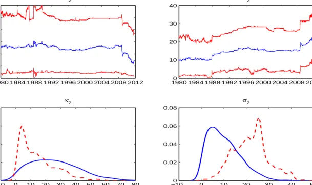
parameter learning in the SE-M3 model. Figure 4 presents the jump intensity-related
parameter learning (κ2 andσ2). We find from the upper panels that credible intervals of
these two parameters are barely narrowing down over time. Only from the 08’s financial
crisis on, we observe a little narrowing-down of their credible intervals, indicating jump
clustering becomes important when incorporating this new information. The lower
pan-els plot the prior and posterior distributions (solid and dashed lines, respectively) of
these two parameters. The dispersions of both priors and posteriors are very big. This
result indicates that the information we have is not enough to well identify these two
parameters.
— Figure 3 around here —
— Figure 4 around here —
C. Volatility and Jump Filtering
Embedded in our learning algorithm is an efficient hybrid particle filter. One merit
of this particle filter is that it can separate positive jumps and negative jumps. This
separation is important from both the statistical and the practical perspectives.
Sta-tistically, it makes our self-exciting models feasible to estimate since both diffusion
volatility and the jump intensity depend only on the negative jump. Practically,
in-vestors are mostly concerned about negative jumps. The ability to disentangle negative
jumps provides us an important tool for risk management.
Figure 5 presents the filtered diffusion volatility and the filtered jump intensity in
volatility and the jump intensity abruptly move up to a high level. However, there are
some important differences between the two state variables. Diffusion volatility is well
identified with a tight 90% credible interval. In contrast, our ability to pin down the
jump intensity is much more limited as we can see that its credible intervals are wide
during crisis periods. Further, there seems to be an abrupt change in the behavior of
this latent factor since the 2008 crisis. Prior to this episode, after widening the credible
intervals of jump intensities during crisis periods, they quickly revert to their long-run
mean, whereas they have remained consistently high and wide since the 08’s financial
crisis. It suggests that as far as the tails are concerned, the recent crisis is special, with
a sustained probability of large extreme events going forward.
We have seen that the parameters driving the jump intensity have large 90% credible
intervals. It is interesting to examine the extent to which these results are due to
pa-rameter uncertainty. For this purpose, Figure 6 depicts the filtered dynamic states when
the full-sample posterior means of the fixed parameters are plugged into the particle
filter. In the case of diffusion volatility (the upper panle), the picture does not change
much, consistent with the relatively tight posteriors on most diffusion parameters. The
only notable difference is a smaller peak around the 1987 crash. This can be explained
by the large uncertainty at this point on the parameter driving the volatility feedback,
σ12. The real-time posterior contains larger values that give rise to a more pronounced
volatility feedback phenomenon. However, when looking at the lower panel, we observe
much larger difference. First, fixing the parameters considerably shrinks the credible
intervals, suggesting that a large part of the uncertainty in jump intensities observed
before in Figure 5 is the result of parameter uncertainty. Second, the peak in jump
intensities in 1987 is bigger than before, a mirror image of what we have observed for
diffusion volatility. Finally, when parameters are fixed, even after 2008, the jump
in-tensities revert back to their long run mean fairly quickly and the credible interval does
not stay wide. Thus, the large uncertainty about the tails in the future seems mainly
related to the lack of precise knowledge about the parameters driving the dynamics of
— Figure 5 around here —
— Figure 6 around here —
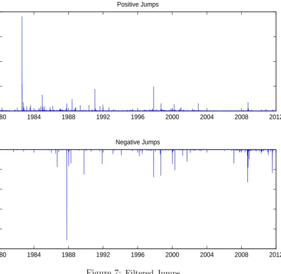
The filtered negative jumps in the lower panel of Figure 7 can effectively capture
all market turmoils such as the 87’s market crash, the 98’s Asian financial crisis, the
08’s financial crisis and the 11’s European debt crisis. However, as shown in the upper
panel of Figure 7, the filtered positive jumps are very small. This is a new and
poten-tially important empirical result, suggesting that whenever jump in volatility is taken
into account, the positive jump component in index returns is not so important and
the positive movements in index returns can be captured by the diffusion component.
This finding reinforces our choice of giving negative jumps more prominence. Similar
implications are also revealed by the SE-M3 model.
— Figure 7 around here —
D. Learning, Volatility Jumps, and Risk Management
Both sequential model analysis and parameter learning point to the fact that the
SE-M1 model and the SE-M3 model are the two best candidates in modeling S&P
500 index returns. Therefore, the following results can be reached. First, diffusion
volatility does jump at the same time as negative jumps in index returns; Second, there
is substantial evidence of jump clustering, in particular after the 08’s financial crisis
even though the jump intensity-related parameters are still hard to be identified.
These results have important implications for risk management. As diffusion
volatil-ity jump is a necessary component in modeling the stock market index and volatilvolatil-ity
co-jumps at the same time as negative jumps in asset returns, traditional hedging
strategies such as only using the underlying assets and/or using both underlying and
derivatives are no longer workable. Furthermore, the big uncertainty in the jump
inten-sity may lead to important risk management implications in the form of substantially
higher tail risk measures.
Here we investigate different Value-at-Risk (VaR) measures implied by our models
Value-at-Risk numbers both for the full sample and the recent financial crisis period,i.e.,
the sample after Lehmans’ bankruptcy on September 15, 2008. We have the following
interesting findings. First, look at the 1% VaR, a frequently used day-to-day measure of
“normal” risk. We find that the difference across the different models in the average VaR
numbers is moderate. They are about -0.024 for the one-day measure and are about
-0.076 for the one-week measure. However, we do observe that the minimum VaR’s
in the full sample are much more extreme for the models with the jump feedback to
diffusion volatility (SE-M1/SE-M3). For example, the minimum one-day VaR’s implied
by the SE-M1 and SE-M3 models are about -0.110, while those impled by the SE-M2
and SE-M4 models are about -0.076. Similar results can also been noticed in one-week
minimum VaR’s. These mainly reflect the fact that the SE-M2 and SE-M4 models
miss the peak in volatility after the 1987 crash. Next, let us check what the 0.1% VaR
numbers convey. These can be interpreted as a measure of tail risk. Here for the full
sample minimum VaR’s we find again large differences across the models but the division
lies between the models with and without self-exciting jumps, i.e., SE-M1/SE-M2 vs.
SE-M3/SE-M4, with the former exhibiting much larger tail risk. For example, the full
sample one-day minimum VaR’s implied by the SE-M1/SE-M2 models are about -0.30,
much larger than those implied by SE-M3/SE-M4 models. Overall these results suggest
that both feedback channels are important but their risk management implications are
somewhat different, with self-exciting jumps exerting their influence deeper in the left
tail.
— Table 5 around here —
5
Concluding Remarks
We introduce a new class of self-exciting asset pricing models where negative jumps play
important roles. Whenever there is a negative jump in asset return, this negative jump
is simultaneously passed on to diffusion variance and the jump intensity, generating
employing a Bayesian learning approach. Using S&P 500 index returns ranging from
January 2, 1980 to October 31, 2011, we find that negative jumps in asset returns lead to
jumps in total volatility mainly through diffusion variance. We find substantial evidence
of jump clustering even though parameters driving the jump intensity remain difficult
to identify. Our results have important risk management implications in practice.
There are several interesting research directions that our results open up. First,
it would be interesting to examine what we can find if option prices are included in
the dataset. This should have the potential to better identify the jump intensity
pro-cess. Second, the sequential nature of our joint parameter and state estimation routine
promises several practical applications like derivative pricing or portfolio allocation.
Appendix A. A Hybrid Particle Filter
The algorithm of the proposed hybrid particle filter consists of the following steps:
• Step 1: Initialize at t = 0: set initial particles to be
{ V1(,i0) =θ1;V (i) 2,0 = 1;J (i) u,0 = 0;Jd,(i0) = 0 }M
i=1 and give each set of particles a weight 1/M;
• Step 2: For t= 1,2, . . . ⋆ IfRt= lnSt−lnSt−τ >0,
– draw Jd,t(i) from its transition law (16);
– draw Ju,t(i) both from its transition law (15) and its conditional posterior
dis-tributionJu,t = lnSt−lnSt−τ−(µ−12V1,t−τ−k(1)V2,t−τ)τ−Jd,t−
√
τ V1,t−τwt,
which is normally distributed. Equal weights are attached to particles
ob-tained from the transition law and the conditional posterior;
– compute the particle weight by
wt(i) = p(lnSt|J (i) u,t, J (i) d,t, V (i) 1,t−τ, V (i) 2,t−τ)p(J (i) u,t|V (i) 2,t−τ) 0.5p(Ju,t(i)|V2(,ti)−τ) + 0.5ϕ(¯µ,σ¯) ,
where ϕ(·,·) represents the normal density with mean ¯µ= lnSt−lnSt−τ −
(µ−12V1(,ti)−τ −k(1)V2(,ti)−τ)τ −Jd,t(i) and standard deviation ¯σ=
√
τ V1(,ti)−τ;
⋆ Otherwise, if Rt= lnSt−lnSt−τ <0,
– draw Ju,t(i) from its transition law (15);
– draw Jd,t(i) both from its transition law (16) and its conditional posterior
dis-tributionJd,t= lnSt−lnSt−τ−(µ−12V1,t−τ−k(1)V2,t−τ)τ−Ju,t−
√
V1,t−τwt,
which is normally distributed. Equal weights are attached to particles
ob-tained from the transition law and the conditional posterior;
– compute the particle weight by
wt(i) = p(lnSt|J (i) u,t, J (i) d,t, V (i) 1,t−τ, V (i) 2,t−τ)p(J (i) d,t|V (i) 2,t−τ) 0.5p(Jd,t(i)|V2(,ti)−τ) + 0.5ϕ(¯µ,σ¯) ,
where ϕ(·,·) represents the normal density with mean ¯µ= lnSt−lnSt−τ −
(µ−12V1(,ti)−τ −k(1)V2(,ti)−τ)τ −Ju,t(i) and standard deviation ¯σ=
√
τ V1(,ti)−τ;
⋆ Normalize the weight: ˜wt(i) =wt(i)/∑Mj w(tj);
• Step 3: Resample (Stratified Resampling)
– Draw the new particle indexes by inverting the CDF of the multinomial
char-acterized by ˜w(ti)at the stratified uniforms i+MU(i) whereU(i) are iid uniforms;
– reset the weight to 1/M;
• Step 4: Update the diffusion variance and the jump intensity particles using (13) and (14), wherezt=ρwt+
√
1−ρ2z˜
twith ˜z being an independent standard
normal noise.
In implementation, when drawing Gamma random numbers, we sample from an
approximate Gamma distribution using proposals from the rejection sampling
the algorithm parallel, instead of rejection sampling, we attach importance weights to
account for the difference between the proposal and the target gamma.
Appendix B. The Marginalized Resample-Move
Ap-proach
As discussed in the text, we have the following recursive relationship between the target
distributions at t−1 and t,
˜
p(Θ, u1:t|y1:t)∝pˆ(yt|ut, ut−1,Θ)ψ(ut|ut−1, yt,Θ)˜p(Θ, u1:t−1|y1:t−1), (26)
from which we can arrive to a set of samples representing the target distribution,
˜
p(Θ, u1:t|y1:t), at time t through the following three steps:
Augmentation Step. For each Θ(n), run the particle filtering algorithm on the new
observation, yt. This is equivalent to sampling from ψ(ut|u (n)
t−1, yt,Θ(n)). Reweighting Step. The incremental weights are equal to ˆp(yt|u
(n) t , u (n) t−1,Θ(n)), leading to new weights s(tn) =st(n−)1×pˆ(yt|u (n) t , u (n) t−1,Θ (n) ), (27)
and the estimated likelihood of the fixed parameters is updated as
ˆ p(y1:t|Θ)(n)= ˆp(y1:t−1|Θ)(n)×pˆ(yt|u (n) t , u (n) t−1,Θ (n)). (28)
Then, the weighted sample
{( Θ(n), u(tn),pˆ(y1:t|Θ)(n) ) , s(tn);n = 1, . . . , N } is distributed
according to our target ˜p(Θ, u1:t|y1:t). The normalized weight is given byπt(n)= s(tn)
∑N k=1s
(k)
t
and the effective sample size is ESSt = ∑N 1 k=1(π
(k)
t )2
observation, essential for model comparison, can be computed as f(yt|y1:t−1) ≡ ∫ p(yt|y1:t−1,Θ)p(Θ|y1:t−1)dΘ ≈ N ∑ k=1 πt(−k)1s(tk). (29)
Notice that the steps so far do not enrich the set of the fixed parameters represented
by the particles. As the target distribution is changing, this will lead to a gradual
deterioration of the performance of the algorithm. To deal with this issue, whenever the
effective sample size falls below some fixed value B1, we implement a resample-move
step in the sense of Gilks and Berzouini (2001) and Chopin (2002). The
resample-move approach is a hybrid of particle methods and MCMC. Here, the population is
first resampled proportional to the weights to multiply particles with high probability.
Then, the set of particles is enriched by passing the particles through a
Metropolis-Hasting kernel that does not change the target distribution, but improves its support
and diversity.
Resample-Move Step. If ESSt < B1, we further consider the following two steps.
(1)Resample the particles proportional toπt(n) and provide an equally-weighted sample
{Θ(n), u(tn),pˆ(y1:t|Θ)(n);n= 1, . . . , N}. (2) Move each particle through a Markov kernel
with a stationary distribution ˜p(Θ, u1:t|y1:t) while the number of unique particles is
below some threshold B2. Here we use marginal particle MCMC kernels from Andrieu
et al (2010) with a proposal distribution of the form
h(Θ, u1:t|Θ′) = ht(Θ|Θ′)ψ(u1:t|Θ), (30)
where ht(Θ|Θ′) is a proposal that can be adapted to the past of the algorithm. For
example, it can be an independent multivariate normal proposal with its mean and
covariance fitted to the sample posterior covariance of Θ. Proposing from ψ(u1:t|Θ)
simply entails the running of a particle filter through the entire data-set at Θ.
The acceptance probability of a new proposed particle (Θ∗, u∗1:t,pˆ(y1:t|Θ)∗) is min { 1; p(Θ ∗)ˆp(y 1:t|Θ)∗ p(Θ(n))ˆp(y 1:t|Θ)(n) ht(Θ(n)|Θ∗) ht(Θ∗|Θ(n)) } . (31)
Notice that we can actually obtain a joint sample fromp(Θ, xt|y1:t) from our learning
algorithm by drawing one particle of the hidden states for each Θ(n) at any time t.
Alternatively, we can use the full particle population and approximate any expectation
E [ f(Θ, xt)|y1:t ] as E [ f(Θ, xt)|y1:t ] ≈ N ∑ n=1 M ∑ i=1 π(tn)f(Θ(n), x(ti,n)). (32) REFERENCES
Ahrens, J.H, Dieter,U. (1974), “Computer methods for sampling from gamma, beta, poisson and bionomial distributions”, Computing 12, 223-246.
A¨ıt-Sahalia, Y., Cacho-Diaz, J., and Laeven, R. (2010), “Modeling Financial Contagion Using Mutually Exciting Jump Processes”, Working Paper.
A¨ıt-Sahalia, Y., and Jacod, J. (2009), “Estimating the degree of activity of jumps in high frequency data”,Annals of Statistics 37, 2202-2244.
A¨ıt-Sahalia, Y., and Jacod, J. (2011), “Testing Whether Jumps Have Finite or Infinite Activ-ity”,Annals of Statistics, 39, 1689-1719.
Andersen, T., Bollerslev, T., Diebold, F.X., and Vega, C. (2007). “Real-Time Price Discovery in Stock, Bond and Foreign Exchange Markets.” Journal of International Economics 73, 251-277.
Andersen, T., Benzoni, L., and Lund, J. (2002). “Towards an Empirical Foundation for Continuous-Time Equity Return Models.” Journal of Finance 57, 1239-1284.
Andrieu, C., Doucet, A., and Holenstein, R. (2010), “Particle Markov Chain Monte Carlo (with Discussions)”,Journal of the Royal Statistical Society: Series B 72, 269-342. Bakshi, G., Cao, C., Chen, Z., 1997. Empirical performance of alternative option pricing
Bandi, F. and Reno, R. (2011), “Price and Volatility Co-jump”. Manuscript.
Barndorff-Nielsen, O., and Shephard, N. (2007), “Variation, Jumps, Market Frictions and High-Frequency Data in Financial Econometrics”, inAdvances in Economics and
Econo-metrics. Theory and Applications, eds. R. Blundell, T. Persson, and W. Newey, New York:
Cambridge University Press.
Bates, David S. (1996), “Jumps and stochastic volatility: Exchange rate processes implicit in Deutsche Mark options”,Review of Financial Studies 9, 69-107.
Bates, David S. (2000), “Post-’87 crash fears in the S&P 500 futures option market”.Journal
of Econometrics 94, 181-238.
Carr, P., Geman, H., Madan, D.B., and Yor, M. (2003), “Stochastic Volatility for L´evy Pro-cesses”, Mathematical Finance 13, 345-382.
Carr, P., and Wu, L. (2004), “Time-changed L´evy Processes and Option Pricing”,Journal of
Financial Economics 71, 113-141.
Carr, P., and Wu, L. (2010), “Leverage Effect, Volatility Feedback, and Self-Exciting Market Disruptions”, Working Paper.
Carvalho, C., Johannes, M., Lopes, H., and Polson, N. (2010), “Particle Learning and Smooth-ing”,Statistical Science 25, 88-106.
Chernov, M., Gallant, A.R., Ghysels, E., and Tauchen, G. (2003), “Alternative Models for Stock Price Dynamics”, Journal of Econometrics 116, 225-257.
Chopin, N. (2002), “A Sequential Particle Filter Method for Static Models”,Biometrika 89, 539-551.
Chopin,N., Jacob, P.E. and Papaspiliopoulos, O. (2011) “ SM C2: A sequential Monte Carlo algorithm with particle Markov chain Monte Carlo updates”, Working Paper
Clark, P.K. (1973). “A Subordinated Stochastic Process Model with Fixed Variance for Spec-ulative Prices.” Econometrica 41, 135-156.
Cont, R., and Mancini, C. (2008). “Nonparametric tests for analyzing the fine structure of price fluctuations”, Working Paper, University of Florence.
Cox, J. C., Ingersoll, J.E., and Ross, S.A. (1985), “A Theory of the Term Structure of Interest Rates”, Econometrica 53, 385-408.
Duffie, D., Pan, J., and Singleton, K. (2000), “Transform Analysis and Asset Pricing for Affine Jump-Diffusions”,Econometrica 68, 1343-1376.
Eraker, B. (2004), “Do Stock Prices and Volatility Jump? Reconciling Evidence from Spot and Option Prices”, Journal of Finance 59, 1367-1403.
Eraker, B., Johannes, M., and Polson, N. (2003), “The Impact of Jumps in Equity Index Volatility and Returns”, Journal of Finance 58, 1269-1300.
Flury, T., and Shephard, N. (2009), “Learning and Filtering via simulation: Smoothly Jittered Particle Filters”, Technical Report, Oxford University.
Fulop, A., and Li, J. (2011), “Robust and Efficient Learning: A Marginalized Resample-Move Approach”, Working Paper.
Gilks, W., and Berzuini, C. (2001), “Following a Moving Target-Monte Carlo Inference for Dynamic Bayesian Models”,Journal of the Royal Statistical Society: Series B 63, 127-146. Gordon, N., Salmond, D., and Smith, A. (1993), “Novel Approach to Nonlinear and
Non-Gaussian Bayesian State Estimation”,IEEE Proceedings-F 140, 107-113.
Heston, S.L., 1993. A closed-form solution for options with stochastic volatility with applica-tions to bond and currency opapplica-tions. Review of Financial Studies 6, 327-343.
Hull, J., and White, A. (1987), “The Pricing of Options on Assets with Stochastic Volatilities”,
Journal of Finance 42, 281-300.
Jacod, J., and Todorov, V. (2010), “Do Price and Volatility Jump Together?”, Annals of
Applied Probability 20, 1425-1469.
Lee, S., and Hannig, J. (2010), “Detecting Jumps from L´evy Jump Diffusion Processes”,
Journal of Financial Economics 96, 271-290.
Liu, J., and West, M. (2001), “Combined Parameter and State Estimation in Simulation-Based Filtering”, In Sequential Monte Carlo Methods in Practice, eds. A. Doucet, N. de Freitas and N. Gordon, New York: Springer.
Madan, D., Carr, P., and Chang, E. (1998), “The Variance Gamma Process and Option Pricing”, European Finance Review 2, 79-105.
Marsaglia, G, Tsang, W.W. (2000), “A simple method for generating gamma variables”ACM
Merton, R.C. (1976), “Option pricing when underlying stock returns are discontinuous”,
Jour-nal of Financial Economics 3, 125-144.
Pan, J., 2002. “The Jump-Risk Premia Implicit in Options: Evidence from an Integrated Time-Series Study”. Journal of Financial Economics 63, 3-50.
Storvik, G. (2002), “Particle Filters for State-Space Models with the Presence of Unknown Static Parameters”,IEEE Transactions on Signal Processing 50, 281-289.
Todorov, V., and Tauchen, G. (2011), “Volatility Jumps”,Journal of Business and Economic
Statistics, forthcoming.
Wu, L. (2011), “Variance dynamics: joint evidence from options and high-frequency returns”,
T able 1: S&P 500 Index Returns and V olatilit y in F our T urbulen t P erio ds P erio d 1 P erio d 2 P erio d 3 P erio d 4 Date Return V ol Date Return V ol Date Return V ol Date Return V ol Oct 16, 1987 -5.30 28.4 Jul 18, 2002 -2.74 28.0 Sep 15, 2008 -4.83 27.4 Aug 4, 2011 -4.90 23.3 Oct 19, 1987 -22.9 82.6 Jul 19, 2002 -3.91 31.0 Sep 16, 2008 1.74 28.0 Aug 5, 2011 -0.06 23.3 Oct 20, 1987 5.20 84.4 Jul 22, 2002 -3.35 32.5 Sep 17, 2008 -4.83 32.4 Aug 8, 2011 -6.90 32.8 Oct 21, 1987 8.71 89.3 Jul 23, 2002 -2.74 33.5 Sep 18, 2008 4.24 35.0 Aug 9, 2011 4.63 36.3 Oct 22, 1987 4.00 89.8 Jul 24, 2002 5.57 38.0 Sep 19, 2008 3.95 37.4 Aug 10, 2011 -4.52 38.9 Oct 23, 1987 -0.01 89.8 Jul 25, 2002 -0.56 38.0 Sep 22, 2008 -3.90 39.6 Aug 11, 2011 -4.53 41.8 Oct 26, 1987 -8.64 94.4 Jul 26, 2002 1.67 38.1 Sep 23, 2008 -1.58 39.9 Aug 12, 2011 0.52 41.8 Note: The table rep orts the S&P 500 index returns and corresp onding v olatilit y , whic h is pro xied b y the standard deviation computed using the previous 22-da y returns at eac h time during the four turbulen t p erio ds including the Blac k Monda y in 1987, the crash of the In ternet Bubble in 2002, the bankruptcy of Lehman Brothers during the global financial crisis in 2008, and the recen t Europ ean debt crisis in 2011. Both returns and standard deviations are in p ercen tage.
Table 2: Summary Statistics of S&P Index Returns
Returns Mean Std. Skewness Kurtosis Min Max 0.078 0.184 -1.193 29.73 -0.229 0.110
ACF ρ1 ρ2 ρ3 ρ4 ρ5 ρ6
-0.028 -0.044 -0.004 -0.015 -0.016 0.008
Note: The table presents descriptive statistics of data for model estimation and empirical analysis. Data are from January 2, 1980 to October 31, 2011 in daily frequency. In total, there are 8,033 observations. Mean and standard deviation are annualized. ρ’s stand for autocorrelations.