Low Complexity Precoding
Schemes for Massive MIMO
Systems
Yulong Chen
School of Engineering
Newcastle University
A thesis submitted for the degree of
Doctor of Philosophy
In order to deal with the challenges of the exponentially growing com-munication traffic and spectrum bands with wider bandwidth, massive MIMO technology was been proposed, which employs an unprecedented number of base station antennas simultaneously to serve a smaller num-ber of user terminals in the same channel. Although the very large antenna arrays for massive multiple-input multiple-output (MIMO) sys-tems lead to unprecedented data throughputs and beamforming gains to meet these data traffic demands, they also lead to prohibitively high energy consumption and hardware complexity. In terms of precoding schemes, the conventional linear precoding entirely processes the com-plex signals in the digital domain and then upconverts to the carrier frequency after passing through radio frequency (RF) chains, which can achieve near-optimal performance with the large antenna arrays. How-ever, it is infeasible because with fully digital precoding, every antenna element needs to be coupled with one RF chain, including the digital-to-analog convertors, mixers and filters, which is accountable for excessively high hardware cost and power consumption. This thesis focuses on the design and analysis of low complexity precoding schemes.
The novel contributions in this thesis are presented in three sections. First, a low complexity hybrid precoding scheme is proposed for the downlink transmission of massive multi-user MIMO systems with a finite dimensional channel model. By analysing the structure of the channel model, the beamsteering codebooks are combined with extracting the
RF precoder, which thereby harvests the large array gain achieved by an unprecedented number of base station antennas. Then a baseband pre-coder is designed based on the equivalent channel with zero forcing (ZF) precoding. In addition, a tight upper bound on the spectral efficiency is derived and the performance of hybrid precoding is investigated.
Second, based on successive refinement, a new iterative hybrid precod-ing scheme is proposed with a sub-connected architecture for mmWave MIMO systems.In each iteration, the first step is to design the RF pre-coder and the second step is to design the baseband prepre-coder. The RF precoder is regarded as an input to update the baseband precoder until the stopping criterion is triggered. Phase extraction is used to obtain the RF precoder and then the baseband precoder is optimized by the orthog-onal property. This algorithm effectively optimizes the hybrid precoders and reduces the hardware complexity with sub-connected architecture. A closed-form expression of upper bound for the spectral efficiency is derived and the energy efficiency and the complexity of the proposed hybrid precoding scheme are analyzed.
Finally, the use of low-resolution digital-to-analog converters (DACs) for each antenna and RF chain is considered. Moreover, in a more practical scenario, the hardware mismatch between the uplink and the downlink for the channel matrix is a focus, where the downlink is not the trans-pose of the uplink in time-division duplex mode. The impact of one-bit DACs on linear precoding is studied for the massive MIMO systems with hardware mismatch. Using the Bussgang theorem and random matrix theorem, a closed-form expression for the signal to quantization, inter-ference and noise ratio with consideration of hardware mismatch and one-bit ZF precoding is derived, which can be used to derive the
achiev-signal-to-noise ratio (SNR) region, which is related to the ratio of the number of base station antennas and the number of mobile users , and the statistics of the circuit gains at the base station.
In conclusion, analytical and numerical results show that the proposed techniques are able to achieve close-to-optimal performances with low hardware complexity, thus the low complexity precoding schemes can be valid candidates for practical implementations of modern communication systems.
First and foremost, I would like to express my sincerest gratitude to my supervisor Prof. Said Boussakta, who has provided me with valuable guidance and unconditional support throughout my years in Newcastle University. I truly appreciate his patience and countless hours he spent with me, discussing my research. I am also thankful to my second super-visor Dr. Charalampos Tsimenidis for his time and great advice during my PhD period. Special thanks are also extended to Prof. Jonathon Chambers for his constructive comments and professional suggestions to my research progression.
I feel very happy to be part of Communications, Sensors, Signal and Information Processing Research Group, the colleagues here are so nice and kind. I would like to thank Zhen Mei, Pengming Feng, Jamal Ahmed Hussein, Wael Abd Alaziz, Achonu Adejo, Jiachen Yin, Yang Sun, Zeyu Fu, Safaa Nash’at Awny, Haicang Li and Yang Xian. The friendship between us is the most unforgettable memory during the past few years in Newcastle.
Additionally, my deepest gratitude is also expressed to my parents for their selfless support and encouragement. Even though we were far apart, their caring warms my heart all the way.
Finally, I would like to express my love to my wife Yu Hong, and my daughter Grace Chen. During my PhD study, my wife has been there for me and gave me all the love. Little Grace is the most precious gift
Contents
List of Figures ix
List of Tables xii
List of Acronyms & Symbols xiii
1 Introduction 1
1.1 Introduction . . . 1
1.2 Motivation and Challenges . . . 3
1.3 Aims and Objectives . . . 4
1.4 Summary of Contributions . . . 5
1.5 Organization of the Thesis . . . 6
1.6 Publications Related to the Thesis . . . 7
2 Literature Review 8 2.1 MIMO Communications . . . 8
2.2 Massive MIMO . . . 10
2.2.1 Multi-user Channel . . . 11
2.2.2 Millimetre Wave Channel . . . 15
2.2.2.1 Propagation Characteristics . . . 17
2.2.2.2 Channel Model . . . 18
2.2.3 Potentials and Challenges . . . 20
2.2.3.2 Challenges . . . 22
2.3 MIMO Precoding . . . 26
2.3.1 Linear Precoding . . . 26
2.3.2 Non-linear Precoding . . . 30
2.3.3 Hybrid Precoding . . . 35
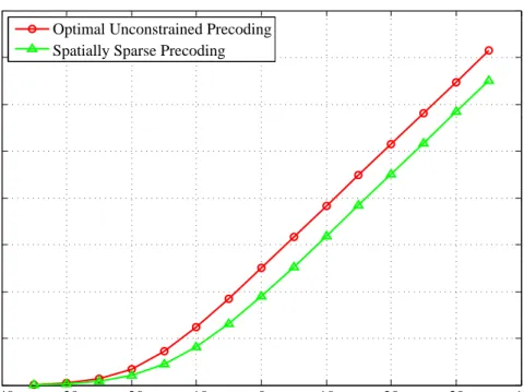
2.3.3.1 Spatially Sparse Precoding . . . 37
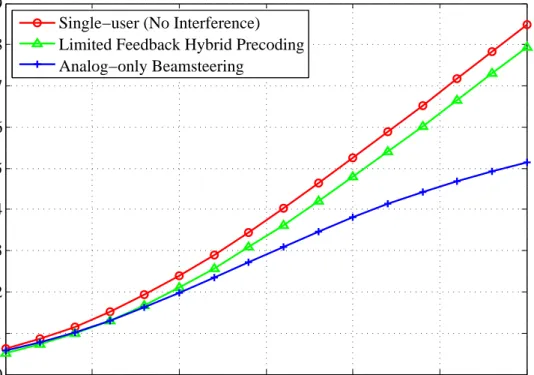
2.3.3.2 Limited Feedback Hybrid Precoding . . . 42
2.4 Summary . . . 45
3 Low Complexity Hybrid Precoding in Finite Dimensional Channel for Massive MIMO Systems 46 3.1 System Model . . . 48
3.2 Channel Model . . . 49
3.3 Proposed Hybrid Precoding Scheme . . . 50
3.3.1 RF Precoder Design . . . 51
3.3.2 Baseband Precoder Design . . . 52
3.4 Analysis of Spectral Efficiency . . . 53
3.5 Simulation Results . . . 56
3.6 Summary . . . 61
4 Energy Efficient Iterative Hybrid Precoding Scheme with Sub-Connected Architecture for Massive MIMO Systems 62 4.1 Introduction . . . 62
4.2 System Model . . . 64
4.3 Channel Model . . . 66
4.4 Problem Formulation . . . 66
4.5 The design of the hybrid precoding with sub-connected architecture . 68 4.5.1 RF Precoder Design . . . 68
4.5.3 Successive Refinement . . . 73
4.6 Analysis of Spectral Efficiency . . . 74
4.7 Energy Efficiency . . . 77
4.8 Analysis of Complexity . . . 78
4.9 Results and Discussion . . . 79
4.10 Summary . . . 86
5 Performance Analysis of Linear Quantized Precoding for the Mul-tiuser Massive MIMO Systems with Hardware Mismatch 87 5.1 Introduction . . . 87
5.2 System Model and Quantized Precoding . . . 90
5.2.1 System Model . . . 90
5.2.2 Linear Quantized Precoding . . . 92
5.3 Analysis of One-bit Quantized Precoding Using Bussgang Theorem . 93 5.4 Analysis of Achievable Rate . . . 96
5.5 Results and Discussion . . . 103
5.6 Summary . . . 109
6 Conclusions and Further Work 110 6.1 Conclusions . . . 110
6.2 Further Work . . . 112
List of Figures
2.1 Point-to-point MIMO system. . . 9 2.2 Multiuser massive MIMO system. . . 11 2.3 The block diagram of TH precoding based on LQ decomposition. . . 31 2.4 The comparison between conventional precoding and hybrid
precod-ing schemes. . . 36 2.5 Spectral efficiency achieved by spatially sparse precoding for mmWave
massive MIMO systems whereNt = 128,Nr = 8, NtRF =Ns = 4. . . . 42
2.6 Spectral efficiency achieved by limited feedback hybrid precoding for mmWave massive MIMO systems where Nt= 64, Nr =K = 4. . . 44
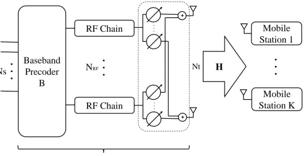
3.1 System diagram of massive multi-user MIMO systems with hybrid precoding for a finite dimensional channel. . . 48 3.2 Spectral efficiency achieved by different precoding schemes with
infi-nite resolution in downlink massive MU-MIMO systems where Nt=
128, K =NRF = 4 and the finite dimension M is 64. . . 56
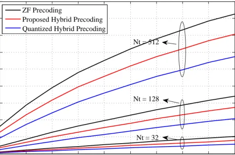
3.3 Spectral efficiency achieved by different quantized precoding schemes with 4 bits of precision in downlink massive MU-MIMO systems where
Nt= 128, K =NRF = 4 and the finite dimension M is 64. . . 57
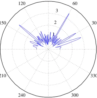
3.4 Spectral efficiency of precoding schemes versus the geometric attenu-ation and shadow fading coefficients. . . 57 3.5 Beam pattern with optimal ZF precoding whereNt= 64, K =NRF =
3.6 Beam pattern with proposed hybrid precoding where Nt = 64, K =
NRF = 4 and SNR is 5dB. . . 59
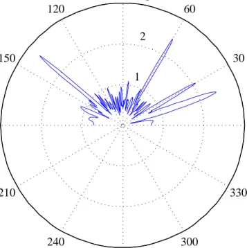
3.7 Beam pattern with quantized proposed hybrid precoding with 4 bits of precision where Nt= 64, K =NRF = 4 and SNR is 5dB. . . 60
3.8 BER comparison of the proposed hybrid precoding with optimal ZF precoding, spatially sparse precoding and limited feedback hybrid pre-coding whereNt = 128, K =NRF = 4 and the finite dimensionM = 16. 61
4.1 Hybrid precoding scheme with sub-connected architecture for mmWave massive MIMO systems. . . 64 4.2 Spectral efficiency achieved by different precoding schemes with
in-finite resolution in mmWave massive MIMO systems where Nt =
128, Nr = 8, NRF = 4. . . 80
4.3 Spectral efficiency achieved by different quantized precoding schemes with 4 bits of precision in mmWave massive MIMO systems where
Nt= 128, Nr = 8, NRF = 4. . . 81
4.4 Spectral efficiency achieved by different precoding schemes with in-finite resolution in mmWave massive MIMO systems where Nt =
128, Nr =NRF= 4. . . 82
4.5 Spectral efficiency achieved by different precoding schemes with in-finite resolution in mmWave massive MIMO systems where Nt =
128, Nr =NRF= 4. . . 82
4.6 The average chordal distance as a function of the number of RF chains where Nt= 120, Nr = 20 and SNR = 0 dB. . . 83
4.7 Energy efficiency of the fully-connected and sub-connected architec-tures against the number of RF chains where Nt= 120, Nr = 20 and
4.8 BER comparison of the proposed hybrid precoding with optimal un-constrained precoding, spatially sparse precoding and SIC-based pre-ocidng where Nt= 128, Nr = 8, NRF= 4. . . 85
5.1 Hardware mismatch for the downlink and uplink transmissions. . . . 90 5.2 Diagram of linear quantized precoding. . . 93 5.3 Achievable rates of one-bit ZF precoding with and without hardware
mismatch, where N = 100. . . 104 5.4 Achievable rates of one-bit ZF precoding with and without hardware
mismatch, where α= 2. . . 104 5.5 Achievable rates of one-bit ZF precoding with hardware mismatch,
where N = 100. . . 105 5.6 Performance approximation of one-bit ZF precoding with hardware
mismatch, where N = 100 and K = 5. . . 106 5.7 Performance approximation of one-bit ZF precoding with hardware
mismatch, where N = 100 and K = 20. . . 107 5.8 SER of unquantized ZF precoding with and without hardware
mis-match, where N = 100. . . 107 5.9 SER of one-bit ZF precoding with and without hardware mismatch,
where N = 100. . . 108 5.10 SER of unquantized and quantized ZF precoding with hardware
List of Tables
2.1 The Comparison of Available Bandwidth at Microwave and MmWave Frequencies . . . 16
List of Acronyms & Symbols
Symbols
(·)∗ Complex Conjugate Operation
(·)H Hermitian transpose of a vector or matrix
(·)T Transpose of a vector or matrix
(·)−1 Inverse of a matrix
∀ For all
= Imaginary component of a complex number
∈ X∈Y indicates that X takes values from the setY
d·e Ceiling Operation
C Set of complex numbers
E[·] Expectation Operation
Q(·) Non-linear quantizer-mapping function
R Set of real numbers
CN(·,·) Complex normal statistical distribution
O(·) Complexity order
M
< Real component of a complex number
σ2
n The variance of the Gaussian noise
IN N byN identity matrix
angle{·} Phase Extraction
det(·) Determinant of a matrix diag(·) Diagonal of a matrix sign(·) Sign of arguments Tr(·) Trace of a matrix
| · | Absolute value of a complex number
k · k2 2 norm of a vector or matrix
k · kF Frobenius norm of a vector or matrix
rank(·) Rank of a matrix
Acronyms/Abbreviations
4G Fourth Generation
5G Fifth Generation
ADE Asymptotic Deterministic Equivalent
BD Block Diagonalization
BER Bit Error Rate
CAGR Compound Annual Growth Rate
CSI Channel State Information
DPC Dirty Paper Coding
FDD Frequency-Division Duplexing
IP Internet Protocol
LTE Long Term Evolution
MF Matched Filter
MIMO Multiple-Input Multiple-Output
MMSE Minimum Mean Square Error
mmWave Millimetre Wave
OFDM Orthogonal Frequency Division Multiplexing
QPSK Quadrature Phase Shift Keying
RF Radio Frequency
SER Symbol Error Rate
SIC Successive Interference Cancellation
SISO Single-Input Single-Output
SNR Signal-to-Noise Ratio
SQINR Signal-to-Quantization-Interference-Noise Ratio
SVD Singular Value Decomposition
TDD Time-Division Duplexing
TH Tomlinson-Harashima
ULA Uniform Linear Array
WiMAX Worldwide Interoperability for Microwave Access
Chapter 1
Introduction
1.1
Introduction
In the past few years, 4G wireless systems, which were standardized in 2012, have provided improved service quality in terms of throughput, spectral efficiency and latency [1]. There are two 4G candidate systems commercially deployed, the Mobile WiMAX 2.0 and the LTE Advanced [1]. The common feature of both candidate sys-tems is that they will provide All-IP connectivity with flexible bit rates and quality of service guarantees for multiple classes of services including voice, mainly using voice over IP, data and video services. This offers theoretical speeds of up to 1.5 Gbps, but the current crop of LTE Advanced networks have a maximum potential speed of 300 Mbps with real world speeds falling a lot lower. With the benefits of 4G networks, wireless internet connectivity will be faster and more affordable. How-ever, with the development of the information and communication technology, recent studies predict that the number of mobile-connected devices is expected to reach 11.6 billion by 2021, including machine-to-machine modules. According to a white paper from Cisco [2], mobile data traffic will grow at a compound annual growth rate (CAGR) of 47 percent from 2016 to 2021, reaching 49 exabytes per month by 2021. Consequently, 5G wireless systems are proposed to deal with the challenges of the exponentially growing communication traffic and spectrum bands with wider
bandwidth [3–5]. In order to achieve high array gain and high spatial multiplex-ing gain, massive MIMO [6–8] employs an unprecedented number of base station antennas simultaneously to serve a small number of single-antenna user terminals in the same channel. Based on the massive MIMO systems, research on hardware complexity and energy consumption has captured the attention of researchers all over the world.
Massive MIMO technology brings huge improvements in spectral efficiency and energy efficiency with the employment of very large antenna arrays at the base sta-tions. Compared with conventional MIMO, massive MIMO can increase the spectral efficiency 10 times or more and simultaneously improve the energy efficiency on the order of 100 times [4]. Additionally, massive MIMO can reduce the latency, simplify the multiple access layer and increase the robustness against interference and inten-tional jamming [4]. Although massive MIMO systems offer huge advantages, there are still challenges ahead for practical implementation, such as hardware require-ments and signal processing [7]. Conventional MIMO systems process the complex signals digitally in the digital domain and then upconvert to the carrier frequency, thus every antenna element needs to be coupled with one RF chain, which includes the digital-to-analog convertors, mixers and power amplifiers. When the number of antennas at the base station is very large, a large number of RF chains will re-sult in excessively high hardware cost and power consumption [9]. Because of these considerations, this thesis focuses on the design of novel hybrid precoding schemes to overcome the constraints of limited number of RF chains. Moreover, in terms of the spectral efficiency, the performance of low complexity precoding schemes is analyzed.
1.2
Motivation and Challenges
With an increase in the number of antennas at the base station, traditional linear precoding schemes such as ZF and minimum mean square error (MMSE) are able to achieve near optimal performance achieved by the dirty paper coding in the downlink communication [6] [8]. However, when the antenna size scales large, traditional schemes require a large number of RF chains. Due to the tremendous number of RF chains, massive MIMO systems will suffer from huge fabrication cost and energy consumption [10]. In order to deal with this problem, cost-effective variable phase shifters are employed to handle the mismatch between the number of RF chains and of antennas. Variable phase shifters with high-dimensional phase-only RF processing are exploited to control the phases of the upconverted RF signal [11–13], which are digitally controlled and changed in a reasonably low time scale for variable channels. Therefore, hybrid precoding schemes are proposed [10,14–16], which exploit a phase-only RF precoder in the analog domain and a baseband precoder in the digital domain. Although the hybrid precoding contributes to reduce power consumption and increase energy efficiency, it leads to the performance degradations. The efficient hybrid precoding schemes should be developed to achieve the best tradeoff between performance and hardware complexity.
Moreover, the millimetre wave (mmWave) frequencies have been put forward as prime candidates for future generation cellular systems, with the potential band-width reaching 10 GHz [17] [18]. Thanks to the decrease in the wavelength of mmWave MIMO systems, the large scale antenna arrays at the transmitters can provide significant beamforming gains to overcome path loss. The hybrid baseband and RF processing is particularly appropriate for mmWave MIMO systems, because the mmWave systems rely heavily on RF processing and the hybrid processing can effectively reduce the excessive cost of RF chains. In order to further reduce the hardware complexity, the number of phase shifters in use can also be reduced. There-fore, the hybrid precoding architectures can be categorized into the fully-connected
and sub-connected architectures [19]. In the fully-connected architecture, each RF chain is connected to all transmitting antennas via phase shifters, while in the sub-connected architecture, each RF chain is sub-connected to only a subset of transmitting antennas [20]. Although the sub-connected architecture sacrifices some beamforming gain, it can significantly reduce the hardware implementation complexity without obvious performance loss.
Likewise, another approach to reduce the power consumption is the use of low-resolution DACs for each antenna and RF chain [21] [22]. The power consumption of the DACs grows linearly with increases in bandwidth and exponentially with the number of quantization bits [23]. With a large number of required DACs in massive MIMO systems, the systems will suffer from prohibitively high power consumption. Therefore, the resolution of DACs must be limited to make the power consumption acceptable. It is worth studying the impact of quantized precoding for the downlink massive MIMO systems.
1.3
Aims and Objectives
The aim of this thesis is to provide a framework to achieve efficient massive MIMO systems with low computational and hardware complexity through the introduc-tion of proposed hybrid precoding schemes. Moreover, the performance of different precoding schemes will be explored and analyzed. The objectives of this thesis are:
• To design the hybrid precoding scheme with fully-connected architecture for the finite dimensional channel in massive MIMO systems.
• To design the hybrid precoding scheme with sub-connected architecture for mmWave massive MIMO systems.
• To analyze the performance of the low complexity precoding schemes in terms of spectral efficiency and bit error rate (BER).
1.4
Summary of Contributions
The contributions of this thesis are focused on the design and performance analysis of novel low complexity precoding schemes for massive MIMO systems. The following list highlights and summarizes the main contributions of this thesis:
In Chapter 3, a low complexity hybrid precoding scheme is proposed for the downlink transmission of massive multi-user MIMO systems with a finite dimen-sional channel model. A tight upper bound on the spectral efficiency is derived and the performance of hybrid precoding is investigated. Simulation results show that the proposed hybrid precoding achieves spectral efficiency close to that achieved by the optimal ZF precoding and performs better than existing hybrid precoding schemes from the literature.
In Chapter 4, based on successive refinement, a new iterative hybrid precod-ing scheme is proposed with a sub-connected architecture for mmWave massive MIMO systems. Then an upper bound on the spectral efficiency is derived with a closed-form expression. The energy efficiency and the complexity of different hybrid precoding schemes are analyzed. Numerical results demonstrate that the proposed hybrid precoding scheme approaches the performance of the optimal unconstrained singular value decomposition (SVD) and has higher energy efficiency and better BER performance than the fully-connected architecture.
In Chapter 5, the impact of one-bit ZF precoding is studied for massive MIMO systems with the uplink and downlink hardware mismatch. The Bussgang theorem and random matrix theorem are used to derive the closed-form expressions for the achievable rate, through the evaluation of expectations and asymptotic deterministic equivalents (ADEs) of a series of random variables. The numerical simulations indicate the validation of the accuracy of the approximation expressions.
1.5
Organization of the Thesis
This thesis is organized as follows:
Chapter 2 provides the background theory and current research related to this work. The fundamentals of massive MIMO are introduced and millimetre wave communications are presented in detail. In addition, a comprehensive survey of the precoding schemes is described, such as, linear precoding, non-linear precoding and hybrid precoding, where the theoretical and methodological contributions to the MIMO precoding are summarized.
Chapter 3 introduces a hybrid precoding design for an M-dimensional channel model. By analyzing the structure of the channel model, the beamsteering code-books are combined with extracting the phase of the conjugate transpose of the fast fading matrix to design the RF precoder. Then the baseband precoder is designed with ZF precoding based on the equivalent channel obtained from the product of the RF precoder and the channel matrix. With perfect channel state information, the spectral efficiency is analyzed and the performance of the proposed hybrid precoding scheme is evaluated in simulation.
Chapter 4 presents an iterative hybrid precoding scheme with a sub-connected architecture. Based on successive refinement, in each iteration, the first step is to design the RF precoder and the second step is to design the baseband precoder. The RF precoder is regarded as an input to update the baseband precoder until the stopping criterion is triggered. Phase extraction is used to obtain the RF precoder and then the baseband precoder is optimized by the orthogonal property. A com-prehensive performance analysis is then carried out in terms of spectral efficiency, energy efficiency and computational complexity.
Chapter 5 studies the impact of one-bit ZF precoding for massive MIMO systems with the uplink and downlink hardware mismatch. With the use of low-resolution DACs for each antenna and RF chain, the hardware complexity can be reduced ef-fectively. Moreover, in more practical scenario, the hardware mismatch is considered
between the uplink and the downlink for the channel matrix, where the downlink is not the transpose of the uplink in TDD mode. Based on these, using the Buss-gang theorem and random matrix theorem, the closed-form analytical expressions are derived for the achievable rate and the performance approximation.
Chapter 6 concludes the thesis and future work in this field is also presented.
1.6
Publications Related to the Thesis
1. Y. Chen, S. Boussakta, C. Tsimenidis, J. Chambers and S. Jin, “Low com-plexity hybrid precoding in finite dimensional channel for massive MIMO sys-tems”, in Proc. 25rd European Signal Processing Conference (EUSIPCO), Kos, Greece, 2017.
Chapter 2
Literature Review
2.1
MIMO Communications
MIMO communication systems were first investigated to focus on point-to-point scenarios. At the transmitter, the serial data is transformed into several parallel data sub-stream and sent by multiple transmit antennas. The multiplex signals received by multiple receive antennas are processed in space and time domain and then switched back to the serial original data at the receiver. The benefits offered by multiple antennas are mainly to harvest the spatial diversity and spatial multiplex-ing gains. The spatial diversity gain aims to enhance the communication reliability by reducing BER [24] [25] and the spatial multiplexing gain contributes to substan-tially increase the communication capacity of the system by multiplexing more data streams [26].
With the development of MIMO communication technology, multi-user MIMO is proposed [27], where a base station equipped with multiple antennas simultaneously communicates with a set of single antenna mobile terminals. In multi-user MIMO scenarios, the base station requires expensive equipment and the mobile terminals can be relatively cheap using single antenna devices. Therefore, multi-user MIMO is more practical to provide the high capacity, increased diversity and interference suppression and being deployed throughout the world.
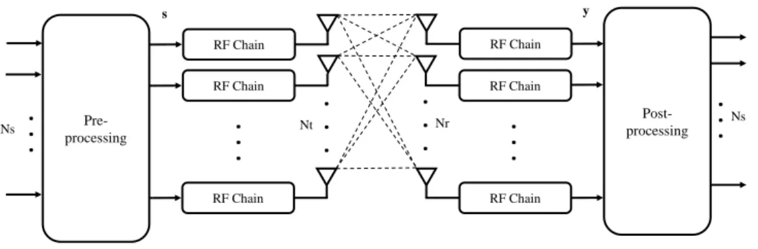
Point-to-point MIMO channel is shown in Fig. 2.1, where the numbers of the transmitter antennas and the receiver antennas are denoted as Nt and Nr,
re-spectively. It is assumed that H ∈ CNr×Nt denotes the channel matrix and n
∼
CN(0, σ2
nINr) represents an additive white Gaussian noise vector with elements
hav-ing zero mean and σ2
n variance. The processed received signal can be written as
y=Hs+n, (2.1)
where y is the CNr×1 received signal vector and s is the
CNt×1 transmitted signal vector. Pre-processing RF Chain Ns
. .
.
Nt. . .
RF Chain.
. .
RF Chain Post-processing RF Chain Ns. . .
RF Chain RF Chain H.
. .
Nr. .
.
s yFigure 2.1: Point-to-point MIMO system.
It is assumed that perfect channel state information is known at both transmitter and receiver sides, the capacity of point-to-point MIMO systems can be expressed as C = log2det I+ Pt Nsσ2n HWHH , (2.2)
where Pt is the total average transmit power, Ns is the number of transmitted
data streams and W is the power allocation matrix. W = diag{w1, w2, . . . , wNt}
with wi being different transmit power. The SVD of the channel matrix is H =
UΣVH [28], where U ∈ CNr×Nr and V ∈
CNt×Nt are unitary matrices and Σ is an Nr×Nt diagonal matrix of singular values λi in descendant order. Therefore,
channels, (2.2) can be written as C= Nmin X i=1 log2 1 + Pt Nsσn2 ˆ wiλ2i , (2.3)
whereNmin =min(Nr, Nt) is the rank of channel matrix and ˆwi is the optimal power
allocation value using the waterfilling algorithm to maximize the system capacity. ˆ wi can be given as ˆ wi = max 0, µ− Nsσ 2 n Ptλ2i , (2.4)
whereµis the waterfilling level, which is chosen to respect the total power constraint.
2.2
Massive MIMO
In recent years, massive MIMO, upgraded from the conventional MIMO technology, has been widely studied to achieve substantial improvements in spectral efficiency and energy efficiency [6] [7]. Massive MIMO was proposed by Thomas L.Marzetta in 2010 [8], which employs an unprecedented number of base station antennas simul-taneously to serve a smaller number of mobile terminals in the same channel. When the number of base station antennas grows asymptotically to infinity, the effects of uncorrelated noise, small-scale fading and intra-cell interference will be eliminated, which makes the channel between the base station and each mobile terminal near-orthogonal. Moreover, large antenna arrays can also achieve large multiplexing and array gains.
Massive MIMO depends on spatial multiplexing, which further relies on the base station to have perfect channel state information, both on the uplink and downlink. Time-division duplex (TDD) is preferred in massive MIMO system, where channel reciprocity can be exploited to get channel state information (CSI) from channel estimation for the uplink. That means the mobile terminals could obtain the same CSI directly for the downlink as it is estimated by using uplink received
pilots. Of course in practical, compared with the downlink CSI, the uplink CSI could be inaccurate or outdated as the channel is fast time-varying, which would affect the performance of the system. Unlike TDD, frequency-division duplexing (FDD), where channel reciprocity cannot be exploitable, is less used. The reason is that the overhead scales linearly with the number of antennas in FDD [29], which makes it difficult to be deployed in massive MIMO system. Nonetheless, FDD mode is still a promising research direction and many researchers have been working on it.
2.2.1
Multi-user Channel
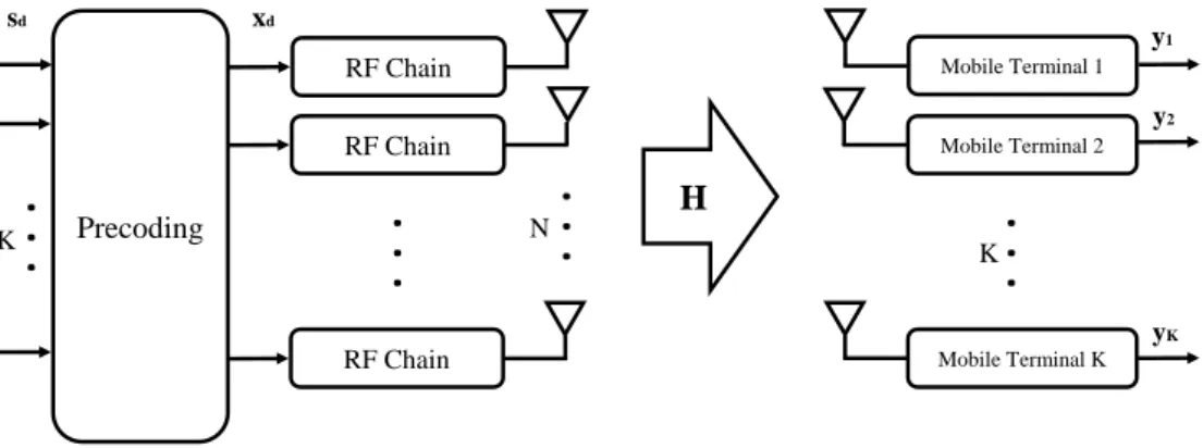
Consider a multi-user massive MIMO system in a single cell scenario shown in Fig. 2.2, where the base station is equipped with N antennas and serves K single-antenna mobile terminals. The channel coefficient is denoted from then-th antenna of the base station to the k-th mobile terminal as hk,n:
hk,n =
p
dktk,n, (2.5)
where dk represents the real large-scale fading coefficients and tk,n represents the
Precoding RF Chain
. . .
N. . .
RF Chain RF Chain Mobile Terminal 1 Mobile Terminal 2 Mobile Terminal K. . .
xd H sd y2 y1 yK. . .
K KFigure 2.2: Multiuser massive MIMO system.
complex small-scale fading coefficients. The large-scale fading accounts for path loss and shadow fading, thus the fading coefficientsD1/2 are assumed to be the same for different base station antennas. The small-scale fading coefficients T are assumed to be different for each mobile terminal and each antenna at the base station. Then,
the downlink channel matrixHfrom the base station to allK mobile terminals can be represented as the product of aK×K diagonal matrixD1/2 and aK×N matrix
T: H=D1/2T, (2.6) where D = d1 d2 . .. dK , (2.7) T= t1,1 · · · t1,N .. . . .. ... tK,1 · · · tK,N . (2.8)
In the downlink transmission, the received signal yd can be written as
yd=√ρdHxd+nd, (2.9)
wherexd= [xd1, xd2,· · · , xdN]T is the vector of the transmitted signal with E[xdxHd] =
IN, nd ∈ CK×1 represents an additive white Gaussian noise vector with elements
having zero mean and unit variance and ρd is the downlink transmit power.
The channel state information is assumed to be known at both base station and mobile terminals. Therefore, in order to maximize the sum transmission rate, the sum capacity of the downlink multi-user massive MIMO systems with power allocations is defined as [4] [30]
C = max
W log2det(IN +ρdH
where W is a positive diagonal matrix whose diagonal elements (w1, w2,· · · , wK)
represent the power allocations for each mobile terminal. The power constraint is denoted as PK
k=1wk = 1. In multi-user massive MIMO systems, the number of
base station antennas N tends to infinity [8], which exceeds the number of mobile terminals. Because the small-scale fading coefficients of T are independent for dif-ferent mobile terminals, the row-vectors of the channel matrix for difdif-ferent mobile terminals are asymptotically orthogonal, hence [31]
HHH =D1/2TTHD1/2
≈ND1/2IKD1/2
=ND. (2.11)
Then the asymptotic sum capacity can be expressed as
C ≈max
W log2det(IK+ρdNWD). (2.12)
For simplicity, matched filter (MF) precoder is used to process the vector of signal for all mobile terminals and the transmitted signal is given by
xd=PD−1/2W1/2sd
=HHD−1/2W1/2sd, (2.13)
where sd∈CK×1 is the vector of source signal and P is the precoding matrix. The processed received signal in (2.9) can be rewritten as
yd=√ρdHHHD−1/2W1/2sd+nd
≈√ρdND1/2W1/2sd+nd. (2.14)
the base station to all mobile terminals can be decomposed to multiple SISO trans-mission. When the power allocation is optimized, the sum capacity can be maxi-mized to achieve capacity optimization.
In the uplink transmission, TDD operation is assumed, thus the uplink channel matrix is the transpose of the downlink channel matrix. The received signal vector
yu can be described as
yu =
√
ρuHTxu+nu, (2.15)
where xu = [xu1, xu2,· · · , xuK]
T is the vector of the transmitted signal from all the
mobile terminals to the base station with E[|xu
k|2] = 1, nu ∈ CN×1 represents an
additive white Gaussian noise vector with elements having zero mean and unit vari-ance and ρu is the uplink transmit power. Assuming that the base station knows
the CSI, the capacity for the uplink is
C = log2det(IK+ρuH∗HT). (2.16)
Based on the result in (2.11), the asymptotic capacity is given by
C ≈log2det(IK +N ρuD) = K X k=1 log2(1 +N ρudk). (2.17)
Due to the asymptotic orthogonality of the channel vectors, MF processing at the base station becomes asymptotically optimal. Therefore, the processed received signal is the product of the conjugate-transpose of the uplink channel matrix and the received signal vector, as
H∗yu =H∗(√ρuHTxu+nu)
From (2.18), the processed received signals from different mobile terminals are effi-ciently and perfectly separated into different streams and the inter-user interference is asymptotically neglected. The signal transmission from each mobile terminal can be considered as a SISO channel with SNR =N ρudk.
2.2.2
Millimetre Wave Channel
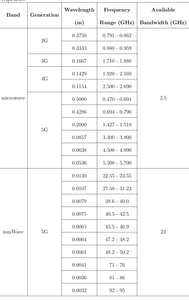
The exponentially growth in communication traffic has exacerbated spectrum con-gestion in current frequency bands, thus new spectrum bands are exploited for future communications. MmWave wireless communications have been demonstrated as a promising approach to solve the spectrum congestion problem, which make the use of spectrum from 30 GHz to 300 GHz [17, 18, 32, 33]. Recent studies show that mmWave frequencies can be used to augment the current microwave frequencies in the range between 700 MHz - 2.6 GHz and the comparison of available bandwidth at microwave and mmWave frequencies is shown in Table 2.1 [34].
On one hand, the use of mmWave frequencies in wireless communications still needs to overcome some technical difficulties. Because of the atmospheric absorp-tion [35], rain attenuaabsorp-tion [36] and low penetraabsorp-tion, the ten-fold increase in carrier frequency will suffer from less favourable propagation loss [34] [37], which is much higher than that of conventional frequency bands. On the other hand, the decreased wavelength of mmWave enables a large antenna array to be packed in small physi-cal dimension [18]. The large antenna array can provide sufficient antenna gain to overcome the severe path loss of mmWave channel. Further, by the use of precod-ing techniques, the large antenna array may support the transmission of multiple data streams to improve spectral efficiency and allow systems to approach capac-ity [10] [38].
In the mmWave systems, due to the practical consideration of the high frequency and bandwidth, there are new constraints on the hardware, such as power consump-tion and circuit technology, which stimulate intensive interest in overcoming these
Table 2.1: The Comparison of Available Bandwidth at Microwave and MmWave Frequencies Band Generation Wavelength (m) Frequency Range (GHz) Available Bandwidth (GHz) 0.3750 0.791 - 0.862 2G 0.3333 0.880 - 0.959 3G 0.1667 1.710 - 1.880 0.1429 1.920 - 2.169 4G 0.1154 2.500 - 2.690 0.5000 0.470 - 0.694 0.4286 0.694 - 0.790 0.2000 1.427 - 1.518 0.0857 3.300 - 3.800 0.0638 4.500 - 4.990 microwave 5G 0.0536 5.500 - 5.700 2.5 0.0130 22.55 - 23.55 0.0107 27.50 - 31.23 0.0079 38.6 - 40.0 0.0075 40.5 - 42.5 0.0065 45.5 - 46.9 0.0064 47.2 - 48.2 0.0061 48.2 - 50.2 0.0041 71 - 76 0.0036 81 - 86 mmWave 5G 0.0032 92 - 95 23
constraints. In order to reduce the number of digital-to-analog converters and their resolutions, the signal processing operations can be partitioned into digital and ana-log domains, which lead to the research on hybrid precoding schemes, beamspace signal processing [39] and low resolution DAC methods. Moreover, since the phase sifters may suffer from quantized phase and insertion loss [40], the performance analysis of the impairments of the analog components and the novel algorithms which can achieve good performance even in presence of impairments are promising research areas.
2.2.2.1 Propagation Characteristics
For mmWave massive MIMO systems with free space propagation, based on the Friis’ Law [41], the ratio between received power Pr and transmitted power Pt is
given by Pr Pt =GrGt λ 4πd 2 , (2.19)
where Gr and Gt are the receive and transmit antenna gains, respectively, λ is the
wavelength and d is the distance between transmitter and receiver. The path loss in (2.19) is given by 16π2(d/λ)2, which implies that if the system is operated at
two different frequencies with the same transmitter and receiver gains, mmWave propagation will experience a higher path loss than conventional lower frequencies. MmWave signals are very susceptible to blockages, because the reduced diffrac-tion and specular propagadiffrac-tion are exhibited in mmWave frequencies, which will lead to a nearly bimodal channel based on the presence or absence of line-of-sight. Due to the sensitivity to blockages, the transmission link can be easily influenced.
However, mmWave frequencies with shorter wavelengths lead to a tremendous increase in the number of antenna elements within the same physical area, which can provide higher array gains to compensate large path loss values. For an N-element uniform linear array (ULA) with constant length L, we define the inter-element
spacing is λ/2, thus the number of elements N can be expressed as
N = 2L
λ . (2.20)
The array gains are proportional to the number of elementsN. Therefore, the higher array gains at high frequencies can compensate for the increased path loss in free space propagation.
The research on mmWave propagation characteristics has captured the attention of researchers over the past years. In small cell scenarios, for distance of up to 200m, the path loss with mmWave frequencies achieves as good performance as conventional cellular frequencies [17, 42, 43], which shows the feasibility of mmWave system in outdoor urban environments. For the urban cellular deployments, the absorption of atmospheric and rain can be beneficial because it further attenuates interference from more distant base stations. In addition, the limitation of mmWave, which can not penetrate brick and concrete, may make the mmWave cells located strictly indoor or strictly outdoor.
2.2.2.2 Channel Model
Due to the high free space path loss, mmWave propagation suffers from the limited spatial selectivity or scattering. The large antenna array is implemented to combat the high path loss, which leads to high levels of antenna correlation. In sparse scattering environments, the large antenna array makes many of the statistical fading distributions used in traditional MIMO analysis inaccurate for mmWave channel. Therefore, a clustered mmWave channel model is introduced to characterize its key features.
When describing the channel model for mmWave systems with Nt transmit and
Nr receive antennas, we generally refer to the array response vectors as a function of
can be given by [14] a(θ) = √1 N[1, e j2λπdsin(θ) , ej4λπdsin(θ),· · · , ej(N−1) 2π λdsin(θ)]T, (2.21)
where λ is the wavelength of the signal and d denotes the distance between any two adjacent antenna elements and θ is the physical angle of arrival or departure. Based on the form of (2.21), the channel matrix is assumed to be the sum of all
Nc scattering clusters, where each cluster contributes Np propagation paths. Under
these circumstances, the mmWave channel model can be defined as [10, 44, 45]
H= s NtNr NcNp Nc X i=1 Np X j=1 βijΛr(θij)Λt(φij)ar(θij)at(φij)H, (2.22)
where βij is the complex gain of the j-th path in the i-th scattering cluster. θij
and φij represent the azimuth angles of arrival and departure, respectively. The
functions Λr(θij) and Λt(φij) are the receive and transmit antenna element gains at
the azimuth angles of θij and φij, respectively. ar(θij) and at(φij) are the receive
and transmit array response vectors at the azimuth angles of arrival and departure. In terms of the Np azimuth angles of arrival and departure in the i-th cluster,
θij and φij are assumed to be randomly distributed with a uniformly random mean
values of θi and φi, respectively. The ranges of θij and φij are defined as [θmin, θmax]
and [φmin, φmax]. In addition, the angular spreads of θij and φij in all clusters are
assumed to be constant with σθ and σφ. The distribution for the angles of arrival
and departure is found that the Laplacian distribution is a good choice to generate all theθij’s andφij’s [46]. Based on these definitions, it is assumed that the transmit
and receive antenna elements are modelled as being ideal sectored elements. Thus, Λt(φij) can be given by [10] Λt(φij) = 1 ∀φij ∈[φmin, φmax], 0 otherwise, (2.23)
and Λr(θij) can be given by Λr(θij) = 1 ∀θij ∈[θmin, θmax], 0 otherwise, (2.24)
where the transmit and receive antenna element gains are unit over the azimuth sectors.
2.2.3
Potentials and Challenges
2.2.3.1 Potentials
1) Massive MIMO has the capability that it can improve the energy efficiency by 100 times and increase the capacity by 10 times or more [47]. In massive MIMO systems, the spatial multiplexing technique leads to the increase in capacity. The improvement of energy efficiency is because the energy can be concentrated in small regions in the space, with the large number of anten-nas. Based on the coherent superposition of wavefronts, after sending out the shaped signals from the antennas, the base station can confirm that all the wavefronts emitted from the antennas will add up constructively at the in-tended terminals’ locations and destructively elsewhere. In order to suppress the interference between mobile terminals, ZF algorithm is used at the cost of increased transmitted power.
Besides ZF, MF is also a good choice for massive MIMO systems, because it reduces the computational complexity with multiplication of the received signals by the conjugate channel responses and is performed in a distributed mode, independently at every antenna element. Although MF performs worse than ZF for the conventional MIMO systems, it works well for massive MIMO systems, because, with large number of base station antennas, the channel responses with different mobile terminals tend to be almost orthogonal. With
MF algorithm, the power can be scaled down as much as possible without seriously affecting the overall spectral efficiency and multi-user interference. Compared to conventional MIMO systems, massive MIMO achieves the overall 10 times higher spectral efficiency, because the systems serve more terminals simultaneously in the same time frequency resource [48].
2) Massive MIMO systems can be built with low-cost and low-power components. In conventional MIMO systems, the base station equips with few antennas, which are fed from high power amplifiers. However, in massive MIMO systems, a large number of antennas lead to hundreds of amplifiers, thus it is infeasible to use high power amplifiers. In order to overcome the problem, the low-cost amplifiers with output power in the milliwatt range are used in massive MIMO systems. Using a large number of antennas, the limits on accuracy and linearity of every amplifier and RF chain are reduced and their combination action becomes more significant. Moreover, the noise, fading and hardware imperfections are averaged with the signals from a large number of antennas combined together in the free space, which increase the robustness of massive MIMO systems.
In addition, in order to reduce the huge energy consumed by the cellular base stations, the renewable resources such as solar or wind can be used to consume less power. If the base stations are deployed to the places where electricity is not available, the renewable resources can be a good choice to address this problem. Along with this, the electromagnetic interference generated by the base stations can also be substantially reduced.
3) Massive MIMO permits a significant decrease in latency on the air interface. When the signal is transmitted from the base station to the terminal, it will travel through multiple paths, which results from the scattering, reflection and diffraction. The fading makes the wireless communication systems suffer
from latency, because the strength of the signal through different paths can be reduced to a considerable low point. If the terminal is trapped in a fading dip, it has to wait until the transmission channel changes until any data can be received. However, in massive MIMO systems, based on the large antenna arrays, beamforming can effectively avoid fading dip and further decrease the latency [4].
Massive MIMO can also simplify the multiple access layer. Thanks to the use of large antenna arrays, the channel strengthens and the frequency do-main scheduling is not suitable. In orthogonal frequency division multiplex-ing (OFDM) systems, massive MIMO provides each subcarrier with the same channel gain, because each terminal can be provided with the whole band-width. Therefore, most of the physical layer control signalling can be redun-dant [4].
4) Massive MIMO increases the strength against the unintended man-made inter-ference and intentional jamming. For the cyber security, intentional jamming is a growing concern. Massive MIMO can provide the methods to improve ro-bustness of wireless communications by the multiple antennas. Massive MIMO also offers an excess of degrees of freedom to cancel the signals from intended jammers. Using joint channel estimation and decoding, massive MIMO sys-tems can reduce the harmful interference by smart jammers, instead of the conventional uplink pilots of channel estimation [47].
2.2.3.2 Challenges
1) Channel State Information Acquisition:
Due to channel estimation and feedback issues, the TDD transmission mode relying on channel reciprocity is regarded almost as a requirement for realistic implementations of massive MIMO systems [49] [50]. Channel reciprocity can be exploited to get CSI from channel estimation for the uplink. That means
the mobile terminals could obtain the same CSI directly for the downlink as it is estimated by using uplink received pilots. Of course in practical, compared with the downlink CSI, the uplink CSI could be inaccurate or outdated as the channel is fast time-varying, which would affect the performance of the system.
Unlike TDD, in the FDD transmission mode, channel reciprocity cannot be exploitable, where the downlink and uplink transmissions operate at different frequencies [51]. Using FDD, the uplink and downlink channels are charac-terized by two separate channel matrices. For the uplink channel estimation, all terminals send different pilot sequences to the base station and the time required for uplink pilot transmission is independent of the number of base station antennas. For the downlink channel estimation, the time required for downlink pilot transmission is proportional to the number of base station an-tennas, because the pilot signals are transmitted from the base station to all terminals first and then all terminals feed back estimated CSI for the downlink channels to the base station. The whole coherence time may be used for the downlink channel estimation, leaving no time for data transmission. There-fore, in massive MIMO systems, the large antenna arrays make the FDD mode infeasible.
However, the research on the FDD transmission has captured the attention of researchers as a very interesting approach in massive MIMO systems. There are several possible methods to enable FDD mode. One way is to design effi-cient precoding schemes based on partial CSI or even no CSI. Another way is to use the idea of compressed sensing to reduce the feedback overhead. There-fore, more investigations of the challenges and feasibility for FDD operation in massive MIMO are needed.
In typical multi-cell massive MIMO systems, the pilot sequences employed by the terminals in adjacent cells may no longer be orthogonal to those within the cell, because the number of orthogonal pilots is smaller than the number of terminals. This inevitably causes interference among pilots in different cells and incurs an ultimate limitation to obtain optimal system performance and sufficiently accurate channel estimation for the uplink, leading to the pilot contamination problem [7]. The channel parameters are estimated from not only the desired link in the target cell but also the interference links in neighbouring cells. The interference rejection performance on massive MIMO systems is challenging in practice due to huge CSI signalling overhead and backhaul signalling latency.
In the multi-cell scenario, it is assumed that the pilot sequence of the k-th terminal in the l-th cell is ψk,l = [ψk,l1 , ψ
2
k,l,· · · , ψ τ k,l]
T, where τ denotes the
length of the pilot sequence. In terms of non-interference between terminals, the pilot sequences employed by the terminals within the same cell and between neighbouring cells are orthogonal, thus
ψk,lHψi,j =δ[k−i]δ[l−j], (2.25) where δ[·] is defined as δ[x] = 1 x= 0, 0 x6= 0. (2.26)
Therefore, the base station can obtain the estimation of the channel matrix without pilot contamination. However, if the period and bandwidth are lim-ited, the number of orthogonal pilot sequences limits the number of terminals that can be served by the multi-cell multi-user systems. In massive MIMO systems, the base stations are expected to serve more terminals, thus
non-orthogonal pilot sequences are utilized in adjacent cells. In this case, suffering from pilot contamination,
ψHk,lψi,j 6= 0. (2.27)
Thus, the estimation of channel matrix will be affected by the non-orthogonal pilot sequences.
Recently, various approaches are proposed to reduce and even eliminate the pilot contamination phenomenon. For example, the efficient channel estima-tion algorithms or blind transmission techniques that circumvent the use of pilots can be used to mitigate the influence of pilot contamination. The pilot contamination precoding is also a promising method to reduce the interference with cooperative transmission.
3) Hardware and Computational Complexity
With hundreds of antennas at the base station, massive MIMO systems require hundreds of RF chains, which include a large number of digital-to-analog con-vertors, mixers and power amplifiers. This leads to huge power consumption, hardware cost and complexity. Therefore, the need for cheaper and low power hardware becomes a significant factor for massive MIMO systems. To re-duce implementation cost and complexity without obvious performance loss, an electromagnetic lens antenna is proposed in [52] [53] to provide spatial multipath separation and energy focusing functions.
In addition, the computational complexity of precoding schemes increases to-gether with the number of antennas at the base station. Therefore, the design of low complexity precoding algorithms is needed in massive MIMO systems, which reduces the time for data transmission. Moreover, the hybrid precoding schemes can also contribute to reduce the hardware complexity by reducing the number of RF chains.
2.3
MIMO Precoding
Precoding is a generalization of beamforming to support multi-stream transmission in multi-antenna wireless communications. In multi-user MIMO systems, precoding techniques are generally preferred for the downlink communications. The precoding techniques are applied at the source signals before they are transmitted which can overcome the interference between mobile terminals. Moreover, because the base station has high computing ability and power supply, precoding is a reliable tech-nique that exploits the channel state information available at the transmitting side in order to be convenient for signal detection at the receiving side, which can reduce the burdens of signal processing and simplify the structure at the mobile terminals. For regular MIMO systems, precoding techniques can be divided into two cate-gories, linear precoding [54–56] and non-linear precoding [57] and there are essential differences between them. Linear precoding has poor performance with low imple-mentation complexity, while non-linear precoding has good performance with high implementation complexity. Theoretical analysis illustrates that the non-linear pre-coding methods such as Dirty Paper Coding (DPC) could achieve the capacity of MIMO Gaussian broadcast channel [58]. In massive MIMO systems, linear precod-ing schemes are shown to be near-optimal with the large antenna arrays. Thus, it is more practical to use low complexity linear precoding techniques in massive MIMO systems. However, the use of linear precoding brings us new problems in massive MIMO systems, which makes the systems suffer from excessively high hardware cost and power consumption. Then we introduce some efficient hybrid precoding schemes to overcome the constraints of hardware complexity.
2.3.1
Linear Precoding
With the perfect CSI known at the transmitter, we define the transmitted signal x
signal can be calculated as
x=Ps, (2.28)
where Pis the precoding matrix. Since the transmitted power is limited by Pt, the
precoding matrix has to be designed to satisfy the transmit power constraint, that is
E[kPsk22] =Pt. (2.29)
Some fundamental linear precoding techniques are introduced for MIMO communi-cations as follows.
MF is the simplest linear precoding scheme to maximize the received SNR, ig-noring multi-user interference. The MF precoding matrix PMF can be computed as
the Hermitian of the channel matrix H,
PMF = 1 βMF HH, (2.30) where βMF= √1P t q
tr(HHH) is a power normalization factor.
In multi-user scenarios, if each terminal is equipped with a single antenna, inter-ferences from other signals cannot be cancelled. In order to deal with the multi-user interference, ZF precoding is widely used. The ZF precoding matrix PZF can be computed as the pseudoinverse of the channel matrix,
PZF = 1 βZF HH(HHH)−1, (2.31) whereβZF = √1Pt q
tr((HHH)−1) is a power normalization factor. ZF precoding
tech-nique is attractive due to their simplicity, however, when the terminals are equipped with multiple antennas, block diagonalization (BD) method is more suitable. It is
defined that the base station with Nt antennas serves K terminals in the
commu-nication systems. The number of antennas for each terminal is Nr. For the i-th
terminal, the received signal yi ∈CNr×1 can be expressed as yi =Hi
K
X
k=1
PBDk xk+ni, (2.32)
where Hi ∈ CNr×Nt is the channel matrix between the base station and the i
-th terminal, PBDk ∈ CNt×Nr is the BD precoding matrix for the k-th terminal, xk ∈ CNr×1 is the source signal vector and ni ∈ CNr×1 is the noise vector. The
equivalent combined channel matrix of all terminals is given by
H= H1 H1 · · · H1 H2 H2 · · · H2 .. . ... . .. ... HK HK · · · HK . (2.33)
Therefore, the received signals for all terminals are written as
y1 y2 .. . yK = H1 H1 · · · H1 H2 H2 · · · H2 .. . ... . .. ... HK HK · · · HK PBD1 x1 PBD2 x2 .. . PBDK xK + n1 n2 .. . nK = H1PBD1 H1PBD2 · · · H1PBDK H2PBD1 H2PBD2 · · · H2PBDK .. . ... . .. ... HKPBD1 HKPBD2 · · · HKPBDK x1 x2 .. . xK + n1 n2 .. . nK . (2.34)
terminal as H−i = [HH1 · · ·HHi−1H H i+1· · ·H H K] H , (2.35) where H−i ∈ C(Nt−Nr)×Nt and N
t = KNr. In order to eliminate the multi-user
interference, BD method is used to make the off-diagonal term HiPBDj in (2.34)
equal to 0Nr×Nr. Thus, (2.35) should be satisfied with the constraint
H−iPBDi =0(Nt−Nr)×Nr, i= 1,2,· · · , K. (2.36)
This implies that the precoding matrixPBDi must be designed to lie in the null space of H−i. With the use of BD, the received signals for all terminals can be rewritten as y1 y2 .. . yK = H1PBD1 0 · · · 0 0 H2PBD2 · · · 0 .. . ... . .. ... 0 0 · · · HKPBDK x1 x2 .. . xK + n1 n2 .. . nK . (2.37)
In terms of the design of BD precoding matrix, it is assumed the rank of H−i is
Nrank =Nt−Nr. The SVD of H−i can be expressed as
H−i =UiΣiVHi =UiΣi V(1)i V(2)i H , (2.38)
whereUi is anNrank×Nrank unitary matrix, Vi is anNt×Ntunitary matrix and Σi
is anNrank×Ntdiagonal matrix of singular values in descendant order. Viis divided
into two parts, V(1)i ∈CNt×Nrank consists of the N
V(2)i ∈CNt×Nr consists of the N
r zero singular vectors. MultiplyingH−i with V
(2) i , H−iV(2)i =Ui Σ(1)i 0 V(1)i H V(2)i H V (2) i =UiΣ (1) i V (1)H i V (2) i =UiΣ(1)i 0 =0, (2.39)
where Σ(1)i is the first partition of dimension Nrank ×Nrank. Thus, V (2)
i forms an
orthogonal for the null space of H−i and PBDi = V(2)i can be used for precoding the signal of the i-th terminal with BD constraint. However, the main computa-tional complexity of BD precoding comes from the SVD operation, which makes the computational complexity increase with the number of terminals and the system dimensions.
2.3.2
Non-linear Precoding
Compared with linear precoding methods, non-linear methods, such as DPC [29], Tomlinson-Harashima (TH) precoding and vector perturbation (VP) offer significant sum-rates benefits, however, with the use of non-linear operations, the systems will suffer from higher implementation complexity.
DPC method was proposed by Costa in 1983, which showed that if the interfer-ence is known to the transmitter, the theoretical channel capacity can be achieved and the effect of the interference can be cancelled. In multi-user systems, when designing precoding matrix for the k-th terminal, the interferences caused by the first up to (k −1)-th terminals are considered to be cancelled. In addition, such remarkable performance can be achieved without the need of additional power in transmission nor of shared CSI with the receiver. However, DPC is infeasible in practical, because it requires infinite length codewords and complicated methods for
signal processing.
TH precoding is an equalization technique originally proposed to cancel the inter-symbol interference. In MIMO systems, TH precoding can be used to eliminate the interference between different sub-channels. Although TH precoding suffers a performance loss compared to DPC, it is feasible to implement in practice instead of DPC method.
mod
τ+
B
-
I
F
+
mod
τn
s
𝒙
r
𝐬
H
G
Figure 2.3: The block diagram of TH precoding based on LQ decomposition.
Fig. 2.3 shows the structure of TH precoding and we assume the numbers of transmitter and receiver antennas are equal to N for simplicity. TH precoding can be implemented on the basis of LQ decomposition, thus, the channel matrix H is decomposed into the multiplication of a lower triangular matrix L and a unitary matrix Q,
H=LQ. (2.40)
A scaling matrix G is defined to contain the corresponding weighted coefficient for each stream. Thus it should have a diagonal structure and the diagonal elements is corresponding to the inverse of the diagonal elements of L, which is given by
G= l−111 0 · · · 0 0 l22−1 · · · 0 .. . ... . .. ... 0 0 · · · l−N N1 , (2.41)
the product of G and L, which is utilized to cancel the interference caused by the previous streams from the current stream. The feedback matrix B is computed as
B=GL. (2.42)
Therefore, the matrixBis a lower triangular matrix with ones on the main diagonal. It is defined the feedforward matrix F as the conjugate transpose of the unitary matrix Q, because the power of the transmitted signal keeps constant using the unitary matrix. The feedforward matrix F is implemented at the transmitter to enforce the spatial causality.
It is assumed thats= [s1, s2,· · · , sN]T is the source signal and ˜x= [˜x1,x˜2,· · · ,x˜N]T
is the pre-signal. Based on the idea of serial interference cancellation, the interfer-ence of the transmit signals can be cancelled and the amplitude of pre-signals can be also limited by modulus operation. The pre-signal ˜x is computed as
˜ x1 =s1 ˜ x2 = modτ[s2−b2,1x˜1] .. . ˜ xi = modτ " si− i−1 X j=1 bi,jx˜j # .. . ˜ xN = modτ " sN − N−1 X j=1 bN,jx˜j # , (2.43)
where bi,j is the element of the matrix B in i-th row and j-th column and modτ
is the function of modulus operation to adjust the transmission power. τ is a real number that depends on the chosen modulation. From (2.43), the i-th terminal needs to cancel the interferences caused by the first up to (i−1)-th terminals, which is similar to DPC method.
With the effect of the modulus operation, a modified source signal can be ob-tained by adding a perturbation vector d to the source signal s, which is given by
v=s+d. (2.44)
Based on Fig. 2.3, the feedback processing is mathematically equivalent to an inver-sion operation B−1, thus the received signal can be expressed as
r=G(HFB−1v+n)
=GHFB−1v+Gn. (2.45)
Finally, the receiver needs to apply an additional modulo operation in order to estimate the received signal.
In addition, [59] proposed a new non-linear precoding method called VP ap-proach. When using VP, a perturbation vector is added to the source signal vector. However, the perturbation vector can not be arbitrary, because this vector is not known to the receivers, thus the receivers cannot eliminate the effect of the pertur-bation effectively. Based on TH precoding, the elements of the source signal are perturbed by an integer, then the effect of the perturbation vector can be elimi-nated by the modulus operation at the receiver. Assume the channel matrix is H
of dimension N ×N and the source signal vector is s of dimension N×1 , and the perturbed signal vector ˜sis written by
˜
s=s+τl, (2.46)
Based on the ZF-VP, the transmitted signalx is given by x= √1 γH H (HHH)−1˜s, (2.47) where γ = kHH(HHH)−1˜sk2
F is the power of the transmitted signal vector. Then
the received signal vector y is expressed as
y=√γ(Hx+n) =√γ(√1 γHH H (HHH)−1˜s+n) = ˜s+√γn, (2.48)
where n is the noise vector. After the received signal is processed by the modulus operation, ignoring the effect of n,
modτ(y) = modτ(s+τl) =s, (2.49)
where τ is a real number that depends on the chosen modulation. Therefore, we can recover the source signal with VP method. From (2.48), √γ is the main factor to design the perturbation vector l. If γ is very large, the system performance will degrades significantly. Thus the transmit power normalization γ is minimized to design the optimal perturbation vector l,
l= arg min l γ = arg min l kH H (HHH)−1˜sk2F = arg min l kH H(HHH)−1(s+τl)k2 F. (2.50)
The choice of l is a N-dimensional integer-lattice least-squares problem, for which there exist a large number of approximate algorithms.
2.3.3
Hybrid Precoding
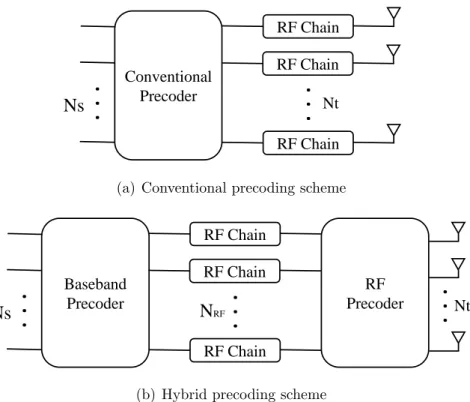
In mmWave MIMO system with a large number of antennas, the conventional linear and non-linear precoding schemes are infeasible, because the system will suffer from prohibitively high energy consumption and hardware complexity. To solve this prob-lem, the hybrid precoding schemes are proposed to reduce the number of RF chains, with cost-effective variable phase shifters employed to handle the mismatch between the number of antennas and RF chains. The comparison between conventional precoding and hybrid precoding is shown in Fig. 2.4, where NRF << Nt. Hybrid
precoding exploits a high-dimensional phase-only RF precoder in the analog domain and a low-dimensional baseband precoder in the digital domain. The transmitted signals are precoded by the baseband precoding first to guarantee the performance, and then precoded by the RF precoding to save the energy consumption and reduce the hardware complexity.
In mmWave massive MIMO systems, [60] and [10] use hybrid methods to obtain near optimal SVD performance, which decompose the optimal precoder and com-biner through the concept of orthogonal matching pursuit. Due to the high complex-ity of searching columns of the overcomplete matrix in [10], a low-complexcomplex-ity hybrid sparse precoding method is proposed in [61] using a greedy method with the element-wise normalization of the first singular vector of the residual. Unlike the point-to-point MIMO systems, the multi-user MIMO systems not only suffer from the noise and inter-antenna interference but are also influenced by the multi-user interference. Thus, the methods above are not suitable for the multi-user scenario. Several hy-brid precoding schemes are proposed to solve the problem. In [14], limited feedback hybrid precoding is proposed with short training and feedback overhead to achieve near optimal block diagonalization performance. A phased ZF precoding in [9] ap-plies phase-only control at the RF domain and then performs a low-dimensional baseband ZF precoding based on the effective channel seen from baseband, which approaches the performance of the virtually optimal full complexity ZF precoding
in a massive multi-user MIMO scenario. Conventional Precoder RF Chain RF Chain Ns
. .
.
. .
.
RF Chain Nt(a) Conventional precoding scheme
Baseband Precoder RF Chain RF Chain Ns
. .
.
NRF. .
.
RF Precoder RF Chain Nt. .
.
(b) Hybrid precoding scheme
Figure 2.4: The comparison between conventional precoding and hybrid precoding schemes.
The precoding schemes above are called fully-connected architecture, which means each RF chain is connected to all base station antennas. When the base station an-tenna number is fairly large, the fully-connected architecture requires a large number of phase shifters for the RF precoder, which leads to both high energy consumption and hardware complexity. In order to further reduce the energy consumption and hardware complexity, the hybrid precoding design with sub-connected architecture is considered in mmWave massive MIMO systems. In the sub-connected architecture, each RF chain is connected to only a subset of base station antennas, instead of all base station antennas. The advantage of the sub-connected architecture is to reduce the number of required phase shifters, which can be more energy-efficient and more practical for antenna deployment. In [19], some hybrid MIMO architectures are pro-posed to reduce the cost, complexity, and power consumption of mmWave MIMO systems, while incurring small loss in the system performance. The constraints on the original hybrid precoding problem with sub-connected architecture is different