An investigation into the effectiveness of sim ulation-extrapolation
for correcting m easurem ent error-induced bias in multilevel models
C hristopher C uster
April 17, 2015
A b s tr a c t
T his p a p e r is an investigation into correcting th e bias introduced by m easurem ent errors into
m ultilevel models. T he proposed m ethod for th is correction is sim ulation-extrapolation (SIM EX ).
T he pap er begins w ith a detailed discussion of m easurem ent error and its effects on p aram eter
estim ation. We th e n describe th e sim u lation-extrapolation m ethod and how it corrects for th e
bias introduced by th e m easurem ent error. M ultilevel m odels and th e ir corresponding p aram eters
are also defined before perform ing a sim ulation. T he sim ulation involves estim atin g th e m ultilevel
m odel p aram eters using our tru e ex p lan ato ry variables, th e observed m easurem ent error variables,
and two different SIM EX techniques. T he estim ates obtained from our tru e ex p lan ato ry values
were used as a baseline for com paring th e effectiveness of th e SIM EX m ethod for correcting bias.
From these results, we were able to determ ine th a t th e SIM EX was very effective in correcting
th e bias in estim ates of th e fixed effects param eters and often provided estim ates th a t were not
significantly different th a n those from th e estim ates derived using th e tru e ex p lan ato ry variables.
random slope variance estim ates, b u t not for th e random intercept variance estim ates. U sing th e
sim ulation results as a guideline, we th e n applied th e SIM EX approach to an o rthodontics d a ta se t
to illu strate th e application of SIM EX to real d a ta .
1
I n tr o d u c tio n
M easurem ent error problem s arise w hen certain variables in a sta tistic a l analysis are m easured
inaccurately. T he tru e value, X t , is often unobserved directly and is instead observed w ith additional
e rro r (Fuller, 1987). T his is a com m on and problem atic source of bias in sta tistic a l models, resulting
in incorrect inferences which can be very costly for th e researcher. For exam ple, m edical and
epidem iological d a ta will often contain m easurem ent erro r and th e inferences o b tained from these
m odels are critical to th e research being perform ed. M easurem ents such as blood pressure and
v itam in levels, am ong m any others, are often m easured w ith erro r and th is m ay cause m isleading
and incorrect results for th e researcher's analysis. T h e inferences m ade from a stu d y of this n a tu re
are obviously incredibly im p o rta n t and need to be as accurate and reliable as possible. From this,
th ere is a need to develop tools and m ethods th a t can overcome th e bias introduced by m easurem ent
error.
In general, sta tistic a l estim ators are desired to contain certain properties, such as being unbi
ased, consistent and m inim al variance. In regression models, for exam ple, p a ra m ete r estim ates are
com puted under th e assum ption th a t ex p lan ato ry variables are m easured w ith exactness. W hen
these variables are m easured w ith error, these estim ators often lose th e ir desirable qualities. In
m any situations, it is im possible to elim inate m easurem ent error and so we need to establish esti
m ators th a t preserve th e desired properties, despite th e additional error.
T his project investigates th e effects of m easurem ent erro r in certain covariates in m ultilevel
We investigate how m easurem ent erro r in level 1 covariates affect th e estim atio n of these fixed and
random effects. In addition, we investigate th e use of a m ethod known as sim ulation-extrapolation
(SIM EX) to correct th e bias introduced by m easurem ent error (Cook and Stefanski, 1994). SIM EX
is a general and widely used m ethod in m easurem ent error m odeling. SIM EX has been shown to
be effective a t correcting bias in a variety of regression models. We have not seen an exam ple of
its application to m ultilevel m odels and so our goal is to investigate th e effectiveness of SIM EX for
p a ra m ete r estim atio n in m ultilevel models.
T his pap er will first provide a m ore in-depth background of m easurem ent error, SIM EX, and
m ultilevel m odels. We describe and rep o rt th e results of a sim ulation designed to investigate th e
effects of m easurem ent erro r and th e SIM EX m ethod in m ultilevel m odels. Finally, we apply SIM EX
to an a ctu al d a ta set as an exam ple of its real world applicability.
2
B a c k g r o u n d
2.1 M e a su r e m e n t error
M easurem ent erro r is a com m on source of bias in m any sta tistic a l analyses, including regression
analysis. In regression models, m easurem ent erro r in covariates can cause bias in estim ated m odel
param eters, and can lead to incorrect inferences. Since th e focus of this stu d y is th e effect of
m easurem ent error on p a ra m ete r estim atio n in m ultilevel models, it is im p o rta n t to first define th e
general effects of m easurem ent error.
In th e classical m easurem ent erro r model, we assum e th a t a variable of interest, X , is m easured
w ith independent, additive erro r having m ean 0. T h a t is, X is m easured as W where
W = X + U, (1)
norm ally d istrib u ted , U ~ N (0, a2a), is also com m only m ade. As will be th e case in our study, it
is also com m on, and often required, th a t aU is known or accurately estim ated when w orking w ith
m easurem ent erro r models.
To exam ine th e im pact th a t m easurem ent error has on estim atio n of p aram eters, we will look at
a few exam ples. Suppose th e random sam ple X 1, . . . , X n is observed as W 1, . . . , W n according to th e
classical m easurem ent erro r m odel in equation (1). F irst consider th e effect of m easurem ent error
on th e estim atio n of a p o p u lation m ean, ^ x . In th e absence of m easurem ent error th e usual sam ple
m ean X is unbiased for ^ x and has variance V ( X ) = a 2/ n . R eplacing th e tru e m easurem ents w ith
th e error-prone m easurem ents yields th e estim a to r W , and it is straightforw ard to show th a t
T his implies th a t while our sam ple m ean rem ains an unbiased estim ato r, its variability is inflated,
and increases as th e variance of th e m easurem ent error, aU, increases.
is an unbiased estim a to r of a 2. W hen X is observed only as W , th e sam ple variance becomes
2 2
E ( W) = ^x and V ( W) = ^ ^
N ext consider estim atin g th e p o p u lation variance, a 2. In th e absence of m easurem ent error, th e
usual sam ple variance,
i=1
i=1
i=1
1 n
T 5"^[(X i — X )2 + 2(Ui — ^ )(X i — X ) + (Ui — U^)]2 n 1
and therefore
E ( s W) = E (sX + 2sx u + s U)
= E (sX ) + 2 E ( s x u) + E (s U )
2 2
= a x + a u
T hus th ro u g h th e in tro d u ctio n of m easurem ent error, we see th a t th e sam ple variance is no longer
unbiased, and th is bias increases as th e m easurem ent error variance increases. It should also be
noticed th a t given th is result, if th e m easurem ent error variance is known, it would be simple
to co n stru ct an unbiased estim ato r, such as <
r
X = sW — aU . It is easy to see th a t E (c
?X) =E (sW — a 2 ) = a X .
Finally, consider estim atio n of th e slope p a ra m ete r in th e sim ple linear regression model. Here
we assum e th a t th e variable X is related to a response Y according to th e m odel
Yi = P0 + @1X i + ei
where th e regression errors ei are independent w ith m ean 0 and c o n stan t variance. Recall th a t in
th e absence of m easurem ent error, / is estim ated by
/5
1 = s xy/sX. U nder very general assum ptionsth is is a consistent (even unbiased) e stim a to r of th e tru e slope. T h a t is,
/ 1 = sj ^ — ax2y = /1
sx ax
A gain suppose th a t X is m easured according to th e classical m easurem ent error model, and fu rth e r
assum e th a t U and e are independent. R eplacing X w ith W , th e estim ate slope becomes
a _ °wy _
/ 1,w — s wy s xy + 2 —= 12 .suy
w w
N ote th a t s xy —P a xy, s uy —P a uy = 0 and sW —P a x + aU. Thus
P a xy a / a x /?1,w---- P 2 , y 2 = / 1
a x + a U Va x + a U
T his effect is known as a tte n u a tio n , causing th e slope to approach zero as th e m easurem ent error
increases (Fuller 1987). From above, we can see again th a t as th e m easurem ent error variance
increases, th e bias increases and th e estim ated slope approaches zero. On th e oth er hand, as th e
m easurem ent erro r variance approaches zero, th e bias approaches zero, as well.
In th e case of known or estim able m easurem ent erro r variance, a consistent e stim a to r of / 1 th a t
relies only on th e observable d a ta is con stru cted as
These sim ple exam ples illu strate some key concepts in m easurem ent error m odeling. F irst and
forem ost is th a t th e m easurem ent erro r creates bias in m ost of our estim ates. T his bias is directly
related to th e am ount of variability th ere is w ithin th e m easurem ent error. As th e m easurem ent
erro r increases, th e bias will increase. However, if th e m easurem ent erro r variance is known, this
bias can be corrected using th e m ethods described above, allowing for consistent and unbiased
estim ato rs using th e observed d a ta , W .
2.2 S IM E X
S im ulation-extrapolation (SIM EX) is a sim ulation-based approach for rem oving th e m easurem ent
erro r bias in p aram etric m odels (Cook and Stefanski 1994). T he m ethod is very general and can
be applied in a wide variety of sta tistic a l analyses including regression m odeling. It is a relatively
sim ple m ethod b u t requires th a t th e m easurem ent erro r variance is known or w ell-estim ated. T he
m ethod uses th e fact illu strated above th a t as m easurem ent error increases, th e bias in th e estim ated
p aram eters increases. T he basic idea of th e m ethod is to first add sim ulated m easurem ent errors
w ith increasing variance to th e d a ta , estim ate th e p a ra m ete r of interest, and determ ine a tre n d
betw een th e resulting estim ates and th e m easurem ent error variance. T he SIM EX estim ate of th e
0, corresponding to th e e stim a to r com puted from d a ta w ith no m easurem ent error, denoted 0true.
Cook and Stefanski (1994) show th a t th is m ethod is equivalent, or asym ptotically equivalent, to
m ethod of m om ents estim ation.
To u n d e rsta n d th e SIM EX process, first define
Wj = X j + Uj
where Wj is our observed variable, X j is our tru e variable, and Uj is our m easurem ent error,
independent of X j , w ith Uj ~ N (0, aU) w here aU is known. N ext, let A > 0 and Z j N (0 ,1 ). Zj
is our ad ditional known m easurem ent error, or pseudo-error, necessary to th e SIM EX estim ation
process. Now define
Wj (A) = Wj + a u ^ A Z j
= X j + Uj + a u \/A Z j
= X j + U j
and th u s U* ~ N (0, aU + AaU). From this, it is easy to see th a t V ar(U *) = (1 + A)aU and so Wj (A)
represents an observation to which additional m easurem ent error is added. If we let
a ( A ) = g(W1 (A ),...,W n(A ))
th e n a (A) represents our p a ra m ete r estim ate for th e given value of A. It follows th a t
Q( —1) ~ ^true
In sim pler term s, by settin g A = —1, we are forcing U* ~ N (0,0) = 0 and th u s Wj = X j , th e tru e
value of our ex p lan ato ry variable.
In order to im plem ent th e SIM EX m ethod, th e following steps should be taken:
2. Using a sim ulation, e stim ate 0(Ak) for each k = 1,..., m
3. P lo t 0(Ak) vs Ak and e x tra p o la te to A = —1 (see Figure 1)
T here are m any ways to accom plish step 2, these steps depending on th e stru c tu re of your
SIM EX estim ates. One key factor in th e process of estim atin g 0(Ak) is th a t it requires m any
estim ated sim ulations for each value of Ak, from which th e m ean of those sim ulated values is used
in th e e x tra p o la tio n process. Cook and Stefanski (1994) suggest using M onte C arlo sim ulation for
th e estim atio n process described in step 2. Specifically for each Ak, a large num ber B of M onte Carlo
replicates are repeated, each resulting in th e estim ate 0j(Ak). T hen th e M onte C arlo e stim a to r of
#(Afc) is
^(Afc) = B E ^^(Afc) (2)
For th e e x tra p o la tio n in step 3, th ey recom m end using one of th ree m ethods to establish th e
tre n d betw een Ak and 0(Ak). T h e first, which is shown as an exam ple in F igure 1, is to fit a linear
regression to describe th e tre n d . T he second m ethod is to use a q u a d ra tic regression for cases where
th e tre n d is curved. T h eir th ird m ethod is for when th e tre n d appears to be nonlinear, and follows
th e form of ^(A) = a + b /(c + A). T h e au th o rs of this m ethod also note th a t w hen th e m eaurem ent
e rro r is norm ally d istrib u ted , each of th e e x tra p o la n ts is exact for certain estim ators. However,
th ey claim th a t even m ore im p o rta n t th a n th e exactness of th e e stim ate is th e fact th a t a t least
one of these e x tra p o la tio n m ethods will provide a sufficiently good estim ate.
2 .3 M u ltile v e l M o d e ls
M ultilevel m odels are extensions of th e sim ple linear regression m odel th a t tre a t m odel coefficients
as random variables instead of fixed effects. These m odels, som etim es referred to as mixed-effect
or hierarchical models, are used when m odeling th e coefficients of a p o p ulation as fixed effects is
scores at age 8 and age 11 from children of different schools across London. These d a ta could be
used to create a sim ple linear regression to predict m a th scores a t age 11 based on age 8 scores.
However, it is also very likely th a t th e tre n d betw een scores differs trem endously am ong schools. A
m ultilevel m odel could be used to allow m odel p aram eters describing th e relationship betw een age
8 and age 11 scores to vary random ly am ong schools. Such a m odel would allow estim atio n of a
general, overall tre n d as well as th e variability of th e tre n d am ong stu d en ts a t different schools. For
exam ple, th e estim ates from this m odel could suggest some tre n d betw een th e two age scores, b u t
th a t th e d a ta also shows a high variability for tren d s am ong schools. Technically, predicted values
could be form ulated from th is m odel, b u t th e variance betw een schools would leave such estim ates
highly suspect.
For this stu d y we will focus on m ultilevel m odels w ith a single ex p lan ato ry variable having a
linear relationship w ith a response. T here are th re e ways to param eterize such models, and those
are referred to as th e random intercept, th e random slope, and th e random slope and intercept
m odels. These are defined as th e ir nam e implies, w ith an intercept th a t has a random com ponent,
a slope th a t has a random com ponent, and a m odel w here b o th slope and intercept contain random
com ponents. For exam ple, th e random slope and intercept m odel is defined as
Yij = (^0 + b0j) + (^1 + b1j )x ij + eij
w here th e random com ponents are typically defined as b0j ~ N (0, ofo) and b1j ~ N (0, a^1). N ote
th a t b0j and b1j are not necessarily independent of one another, th u s we define cov(b0j , b1j) = a b01.
Let i = 1, 2, . . . , m be defined as th e num ber of level 1 units, and j = 1,2, .. ., n be defined as th e
num ber of level 2 units. Level 1 units are defined as those clustered w ithin each level 2 u nit. For
our school exam ple, level 1 units would be each stu d e n t and level 2 u n its would be each school
(G oldstein 1999). If th e random com ponents are defined as above, th e n th e exected value of Y is
com ponents, b0 and b1, describe th e variability of th e intercepts and slopes across level 2 units,
respectively, around th e po p u latio n averages.
To relate th is back to th e m a th scores exam ple, using a random slope and intercept m odel
suggests th a t th ere is variability from th e p o p u lation in b o th th e intercept and slope for each
school. T he fixed effects retu rn ed from th e fitted m odel would represent th e estim ated intercept
and slope for th e p o p ulation of schools sam pled. T he random com ponents would represent how
m uch each school’s intercept and slope vary from th e population. If th e schools’ intercept and
slope ten d to show large deviations from th e population, th e n we would expect th e fitted m odel
to re tu rn large variance estim ates for our random effects. T he fitted m odel will also e stim ate th e
covariance betw een th e random com ponents. This would allow us to in te rp re t th e relation betw een
our random variances. A large positive covariance would suggest th a t if we see an increase in th e
v ariability of our intercepts, we should expect to see an increase in th e variability of our slopes. J u s t
as in sim ple linear regression, m easurem ent error is problem atic in m ultilevel m odeling (G oldstein
1995).
3
S im u la tio n
We perform ed a sim ulation stu d y to determ ine th e effectiveness of th e SIM EX m ethod for correcting
covariate m easurem ent error-induced bias in p a ra m ete r estim atio n for m ultilevel models. T he m ain
objective of our sim ulation stu d y was to u n d e rsta n d if and when th e SIM EX m ethod produces
im proved p a ra m ete r estim ates in m ultilevel models, com pared to estim ates th a t ignore m easurem ent
e rro r in th e covariate.
D a ta for sim ulations were generated as follows. F irst tru e values of th e covariate X j were set
covariates, W ij, were generated according to th e classical m easurem ent error model. Specifically,
Yij = (^0 + b0j) + (^1 + b1j ) X ij + eij (3)
Wij = X i j + Uij (4)
where eij ~ N (0, ct;?), b0j ~ N (0, ct20), and b1j ~ N (0, ct^). T h e p aram eters of interest to our study
are th e fixed intercepts and slope, 0 0 and ^ 1, and th e corresponding random com ponents’ variance,
a “20 and ct^1. T he values of these p aram eters were held co n stan t for all sim ulated d a ta se ts, w ith
0 0 = 2, ^ 1 = 3, ct20 = 16, ct21 = 25, and = 6.25. T he tru e values of th e e x p lan ato ry variable, X ,
were defined sim ply as a sequence of 1 to m , w here m was defined as th e num ber of level 1 units.
T his sim plistic approach was used to lim it th e v ariation in th e tru e values so th a t th e effects of th e
m easurem ent erro r variance would be m ore easily observed.
Four sets of pa ra m ete r estim ates were com puted for each sim ulated d a ta set. T hese were th e tru e
estim ates, naive estim ates, SIM EX using linear e x tra p o la tio n (linear SIM EX), and SIM EX using
q u a d ra tic e x tra p o la tio n (q u ad ratic SIM EX ). T he tru e estim ates were estim ated m odel p aram eters
calculated using th e tru e values of th e e x p lan ato ry variable, in o th er words, w ithout m easurem ent
error, X ij . T he naive estim ates were calculated using th e e x p lan ato ry variable w ith m easurem ent
error, W ij, b u t ignore th is fact and include no a tte m p t to fix th is bias. T he two SIM EX estim ators,
w ith linear and q u a d ra tic e x tra p o la tio n techniques, were th e n used to a tte m p t to fix th is bias and
retu rn ed th eir own respective estim ates. All estim ated m odel p aram eters were com puted using th e
lm e r function in R (B ates et al. 2014).
We investigated th e effects of th re e different factors on th e perform ance of these estim ators. These
factors were th e reliability ratio, th e num ber of level 2 units and th e num ber of level 1 units. We
describe each of these factors next.
Since th e im pact of m easurem ent erro r is driven by its variance, th e m ain focus of th e sim ulation
variance. In our sim ulation, we selected th re e levels of reliability ratios to apply to th e m odeling
process. R eliability ratio is defined as
2 / ( 2 , 2\ K a x/ ( a u + a x )
w here aU is th e m easurem ent erro r variance and axX is th e variance of our tru e ex p lan ato ry vari
able. Since our tru e ex p lan ato ry variable, X , was co n stan t th ro u g h o u t th e sim ulation process, its
variance rem ained co n stan t and thus by changing th e reliability ratio, we effectively changed th e
m easurem ent error variance. E xam ining th e form ula above reveals th a t th e reliability ratio and
m easurem ent erro r variance have an inverse relationship. T his an increase in our ratio results in a
decrease in our m easurem ent erro r variance. T he reliability ratios selected for th e sim ulation were
0.75, 0.85, and 0.95.
T he next two variables th a t were altered for th e sim ulation were th e num ber of level 2 units
and th e num ber of level 1 units. It is well-known th a t sam ple sizes can influence th e results of a
sta tistic a l analysis. Since a m ultilevel m odel has essentially two different sam ple sizes, b o th were
deem ed as im p o rta n t factors to vary across th e sim ulation and observe how th ey affect th e SIM EX
estim ates. T he num ber of level 2 units in th e sim ulation were 5 and 30. T he num ber of level 1
u nits were 10 and 60.
For each com bination of n , m , and k, and using th e m odel defined in (3), a d a ta s e t was created
w ith n groups and m subjects w ithin each group. U nder each one of these com binations, 125 ite ra
tions of th e sim ulation were com pleted, resulting in 125 sets of p a ra m ete r estim ates for each of th e
four estim atio n m ethods. For th e two SIM EX estim ators, we defined A = (0 ,0 .1 5 ,0 .2 5 ,0 .5 ,0 .7 5 ,1 ).
It should be noted th a t when A = 0, we are sim ply referring to our observed variable, W , which
was already used to fit th e naive m odel. T hus in our a ctu al SIM EX process, we only applied th e
o th er five values. T he M onte C arlo step in equation (2) was com pleted using B = 50 M onte Carlo
A. Using these m ean values, two regression m odels, a linear and a qu ad ratic, were fit for each esti
m ated p a ra m ete r to describe th e tre n d of 0(A) over A. E ach of these m odels were th e n ex tra p o la ted
backw ards to A = —1 to give an estim ated $true for each p aram eter. T hus, after every sim ulation
iteratio n , we are left w ith 125 estim ates from each of th e four fitted m odels for each of th e four
p aram eters for each of th e twelve factor com binations. T hese estim ates were used to sum m arize
and com pare th e d istrib u tio n for each estim atio n m ethod. T his was accom plished by calculating
th e m ean, bias, variance, and m ean squared error. W hile we recognize th a t m ost sim ulations use a
m uch larger num ber of iterations, this process was very com puter intensive and constrained by th e
available technology. T he next section describes th e results of th is sim ulation.
3.1 R e su lts
T he sim ulation provided some valuable insights in regards to th e effectiveness of th e SIM EX m ethod.
O ur analysis of these results will focus on th e influence th a t th e th re e factors had on bias. Refer to
F igure 7 for a full sum m ary of th e results, including variance of th e estim ates and m ean square error.
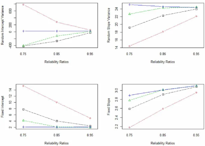
One m ajor, and obvious, result from th e sim ulation is how poorly SIM EX perform ed in estim atin g
th e random intercept variance, aX0. As F igure 7 reveals, along w ith Figures 2-4, th e m ajo rity of
th e estim ates for b o th th e linear and q u a d ra tic approach retu rn ed negative values. W ith th is flaw,
th e estim atio n of th e random intercept variance will not be discussed in th e analysis of th e results,
and instead we will save it for th e conclusion and discuss possible im provem ents. In our discussion,
we define a m ethod as b e tte r if it produces a sm aller bias.
T he sim ulation suggests th a t th e q u a d ra tic SIM EX is th e m ost effective m ethod for correcting
m easurem ent erro r bias. Since th e q u a d ra tic fit appears to be a t least as good as th e linear fit,
and usually b e tte r, th e analysis will focus on th e q u a d ra tic SIM EX m ethod. F irst, le t’s exam ine
am ong m ean estim ates for each of th e four p aram eters across th e th re e different levels of reliability.
From these plots, it is ap p a re n t th a t as reliability ratio decreases, and th u s m easurem ent error
increases, th e SIM EX m ethod perform s significantly b e tte r th a n th e naive estim ato r. W elch’s t-
te sts were perform ed to determ ine if th e observed differences were statistically significant. W hen
com paring th e fixed slope estim ates a t th e reliability ratio 0.95, none of th e four m ethods produce
significantly different results (p > 0.05). For a reliability of 0.85, th e SIM EX q u a d ra tic m ethod
produces a significantly b e tte r result th a n th e naive estim a to r (p « 0), while not being significantly
different th a n th e tru e estim a to r (p = 0.50). T he q u a d ra tic SIM EX and tru e estim ato rs were also
found to not be significantly different at a reliability level 0.75 (p = 0.13). For th e random slope
and fixed intercept estim ates, th e te sts show th a t th e q u a d ra tic SIM EX m ethod is significantly
b e tte r th a n th e naive m odel across all levels of reliability ratios (p < 0.05) and only outperform ed
by th e tru e estim ates a t a reliability ratio of 0.75 (p & 0).
A nalyzing th e results w ith respect to num ber of level 2 u n its sam pled shows sim ilar tren d s
betw een estim atio n m ethods, th ough it reveals th a t th e num ber of u n its does not seem to have
an effect. F igure 3 shows th a t as we increase from 5 to 30 units, our estim ates ten d to stay th e
same. Again, W elch’s t-te sts were used to te st for significant differences betw een th e m ethods.
At a significance level 0.05, th e SIM EX q u a d ra tic estim atio n m ethod produced significantly b e tte r
results th a n th e naive estim ato r. T here was also found to be no significant difference betw een th e
SIM EX q u a d ra tic and th e tru e estim ates for th e fixed slope a t b o th level 2 u n it sam ple sizes, as
well as not being different for th e random slope estim ates at a sam ple size of 5.
T he final step in th e analysis was to exam ine th e effects of level 1 sam ple sizes on our estim ates.
Figure 4 shows th a t th e num ber of level 1 sam ples did not have a large influence on th e random and
fixed slope estim ates, b u t did significantly increase th e bias in th e fixed intercept estim ates for th e
where a t a significance level 0.05, th e q u a d ra tic SIM EX m ethod was significantly b e tte r th a n th e
naive m ethod (p « 0). It was also observed th a t th ere was no significant difference betw een th e
q u a d ra tic SIM EX and tru e estim ates for each p a ra m ete r a t a level 1 sam ple size of 10 and th e fixed
slope effect w ith sam ple size 60 (p > 0.05).
4
D a t a A n a ly s is E x a m p le
T he SIM EX m ethod was used to analyze a d a ta se t as an exam ple for how one would apply it to real
d a ta . T he selected d a ta was from an o rthodontics stu d y which involved th e m easure of distance
(m m ) betw een th e center of th e p itu ita ry to th e pterygom axillary fissure. T h e m easurem ents were
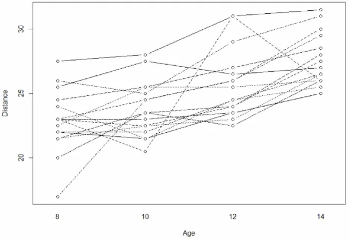
tak en from 16 m ale children at ages 8, 10, 12, and 14 years old. F igure 5 provides a plot of th e
d a ta , w here each line represents a level 2 u n it and each point is a level 1 unit. Specifically for this
exam ple, each child is a level 2 u n it and each to o th m easurem ent is a level 1 unit.
T he m easurem ent error introduced here is th e result of rounding th e age to an integer. Before
th e analysis, th ere are several assum ptions th a t should be noted in order to use this d a ta se t. T he
first is th a t despite th is being a rep eated m easures study, we will ju s t assum e th a t th e errors betw een
level 1 u n its w ithin a level 2 u nit are independent. T he second is th a t th e ages are rounded to th e
closest birthday, and not ju s t th e c u rren t age class. For exam ple, someone 3 m onths away from
tu rn in g 10 will be considered 10 and not 9 as is th e usual case. This allows us to th e n assum e th a t
th e m easurem ent errors have a m ean of 0. We will also assum e th a t these m easurem ent errors,
U , are norm ally d istrib u ted as defined in eq u ation (1) T he final assum ption for th is d a ta is th a t
th e reliability ratio is 0.9. T he observed variance for age is approxim ately 5, th u s our estim ated
m easurem ent erro r variance is 0.866.
T he first step was to fit th e naive model, ignoring th e m easurem ent error. T h e naive p aram eter
m ethod, again using 50 repetitions for th e sim ulation of each of our 5 A values. F igure 6 shows th e
four SIM EX plots used to fit th e m odels and create th e SIM EX prediction, ju s t as in F igure 1.
Since our sim ulation suggested th a t th e q u a d ra tic fit provided th e b e tte r estim ates, we used
th a t sam e m ethod here. From th e q u a d ra tic SIM EX m odel, th e p a ra m ete r estim ates are <r20 =
18.85, (?21 = —0.025, /30 = 15.092, and /31 = 1.328. T he im p o rta n t result here is th a t th e estim ate
of th e fixed slope has increased in value from th e naive estim ate. Know ing th a t m easurem ent
e rro r causes an a tte n u a tio n bias, th e fact th a t th e SIM EX m ethod has increased th e value of th e
estim ated slope suggests th a t SIM EX was successful in correcting for th e m easurem ent erro r bias.
Also of interest is th a t in th is exam ple it was th e random slope variance th a t predicted a negative
value, in co n tra st to th e sim ulation producing negative estim ates for th e random intercept variance.
One possible ex p lanation is th a t random slope variance is very close to zero, suggesting th a t there
is very little variation of slopes am ong level 2 units. T his possibly lead to th e poor estim ation
results from th e SIM EX process. B ased on our sim ulation and contingent on our assum ption, we
claim th a t these SIM EX estim ates provide less biased results th a n th e naive estim ates and th u s a
b e tte r u n d erstan d in g of th e relationship betw een age and distance.
5
C o n c lu sio n
T h rough this study, we were able to evaluate th e effectiveness of th e SIM EX m ethod for correcting
bias in a m ultilevel model. B ased on th e results of th e sim ulation, it appears th a t SIM EX is a
valid and useful tool for establishing statistically sound p a ra m ete r estim ates. Though, as seen in
th e ap p earance of negative variance estim ates in b o th our sim ulation and d a ta analysis exam ple,
fu rth er research is needed to enhance th e way SIM EX creates these estim ates to prevent such errors
from occurring. F u tu re research should also look to expand on th e m ultilevel m odels being studied,
6
A c k n o w le d g m e n ts
I would like to th a n k my advisor, D r. Julie M cIntyre, for all th e knowledge and assistance provided
during this project, as well as being an integral p a rt of my g rad u a te education. I also would like to
th a n k D r. R on B arry, Dr. Lubov Zeifm an, and D r. M argaret Short for th e ir role in th e com pletion
of th is project and in my o u tsta n d in g education obtained a t th e U niversity of Alaska.
7
R e fe r e n c e s
B ates D, M aechler M, Bolker BM and W alker S (2014). lme4: L inear mixed-effects m odels using
Eigen and S4. ArXiv e-print; su b m itte d to Jo u rn a l of S tatistical Software, U R L :h ttp ://a rx iv .o rg /a b s /1 4 0 6 .5 8 2 3 .
Cook, J., and Stefanski, L. (1994). S im u lation-E xtrapolation E stim atio n in P a ram e tric M easure
m ent E rro r M odels. Jo u rn a l of th e A m erican S tatistical A ssociation, 1314-1314.
G oldstein, H. (1995). C h a p te r 2: T he basic linear m ultilevel m odel and its estim ation. In M ulti
level sta tistic a l m odels (2nd ed.). London: E. Arnold.
G oldstein, H. (1995). C h a p te r 10: M ultilevel m odels w ith m easurem ent error. In M ultilevel s ta tis
tical m odels (2nd ed.). London: E. Arnold.
8
F ig u r e s
Fi xe d In te rc e p t R an do m In te rc e p t V a ri a n c e 0.7 5 0.3 5 Reliability Ratios 0.9 5 co E 0.75 0 .3 5 Reliability Ratios 0.9 5 0.7 5 0.3 5 Reliability Ratios 0.9 5 0.75 0 35 Reliability Ratios 0.9 5
Figure 2: P a ra m e te r estim ates for each m ethod across each level of reliability ratio.
+ tru e estim ate
A q u a d ra tic SIM EX
□ linear SIM EX
Fi xe d In te rc e p t R an do m In te rc e p t V a ri a n c e -i- i ia n c e 24 1 1 A -> ^ CL) CM _ CM Q_ O □ --+ --- 4- GO -A -1 R -c 03 _ DU o ---□ ... - - - ...- u 9? — 30 6 30
Level 2 S am ples Level 2 Sam ples
5 30 5 30
Level 2 S am p les Level 2 S am ples
F igure 3: P a ra m e te r estim ates for each m ethod across each Level 2 sam ple size.
+ tru e estim ate
A q u a d ra tic SIM EX
□ linear SIM EX
Fi xe d In te rc e p t R an do m In te rc e p t V a ri a n c e co E 10 60 10 60
Level 1 S am ples Level 1 Sam ples
10 60 10 60
Level 1 S am p les Level 1 S am ples
F igure 4: P a ra m e te r estim ates for each m ethod across each Level 1 sam ple size.
+ tru e estim ate
A q u a d ra tic SIM EX
□ linear SIM EX
D is ta n ce 8 10 12 14 Age Figure 5: O rth o d o n tist d a ta
0. 03 6 0. 04 0 0. 04 4 0. 04 8 0. 65 0. 70 G .7 5
Random Intercept (b0=16) TRUE Naive Sim ex.Linear Sim ex.Q uadratic N.Group N .Sam ple RR Estim ate Bias V ariance Estim ate Bias V ariance Estim ate Bias V ariance Estim ate Bias Variance
5 10 0.95 14.51 -1.49 148.31 17.89 1.89 234.70 12.35 -3.65 353.48 17.25 1.25 617.31 0.85 16.73 0.73 186.65 36.42 20.42 1380.54 6.31 -9.69 1423.41 9.47 -6.53 4099.33 0.75 17.40 1.40 201.49 55.96 39.96 2694.94 -7.94 -23.94 4048.77 -7.54 -23.54 11759.22 60 0.95 15.03 -0.97 127.09 83.13 67.13 18557.68 -71.46 -87.46 6741.38 -23 .1 0 -39.10 30980.53 0.85 15.06 -0.94 107.70 517.83 501.83 135778.54 -523.02 -539.02 169128.27 -246.31 -262.31 2 29773.34 0.75 16.34 0.34 123.26 1606.83 1590.83 1737516.06 -878.85 -894.85 769501.22 -764.61 -780.61 1184971.46 30 10 0.95 16.49 0.49 26.03 17.29 1.29 52.52 15.85 -0.15 91.83 18.76 2.76 167.07 0.85 16.17 0.17 23.42 26.39 10.39 173.20 -7.88 -23.88 243.77 8.48 -7.52 1163.20 0.75 14.98 -1.02 23.91 55.38 39.38 688.80 -17.56 -33.56 635.42 -17 .0 6 -33.06 3218.05 60 0.95 16.03 0.03 21.43 73.53 57.53 1076.79 -91.48 -107.48 1483.39 11.11 -4.89 10216.05 0.85 16.32 0.32 13.53 530.35 514.35 42583.45 -560.57 -576.57 40311.84 -273.29 -289.29 154022.76 0.75 16.08 0.08 18.10 1412.09 1396.09 183451.82 -756.87 -772.87 70937.47 -805.24 -821.24 3 83572.00
Random Slope (b1=25) TRUE Naive Sim ex.Linear Sim ex.Q uadratic
N.Group N .Sam ple RR Estim ate Bias Variance Estim ate Bias V ariance Estim ate Bias V ariance Estim ate Bias Variance
5 10 0.95 25.12 0.12 322.75 22.88 -2.12 270.79 24.59 -0.41 314.37 25.10 0.10 364.68 0.85 24.03 -0.97 290.00 18.43 -6.57 189.24 22.52 -2.48 296.57 24.99 -0.01 396.31 0.75 23.83 -1.17 304.20 14.38 -10.62 134.25 19.04 -5.96 241.75 22.67 -2.33 429.43 60 0.95 23.43 -1.57 338.67 21.02 -3.98 263.50 22.89 -2.11 310.43 23.34 -1.66 329.85 0.85 24.61 -0.39 213.11 17.92 -7.08 115.04 22.12 -2.88 176.19 23.97 -1.03 207.79 0.75 27.56 2.56 442.01 15.57 -9.43 142.80 20.83 -4.17 256.01 24.55 -0.45 355.19 30 10 0.95 23.79 -1.21 40.63 21.75 -3.25 32.67 23.50 -1.50 37.19 24.26 -0.74 54.78 0.85 24.43 -0.57 46.24 17.90 -7.10 27.31 22.00 -3.00 44.01 23.64 -1.36 57.70 0.75 25.06 0.06 35.78 14.19 -10.81 13.17 18.75 -6.25 24.55 21.89 -3.11 39.82 60 0.95 25.20 0.20 32.92 22.77 -2.23 26.76 24.83 -0.17 31.69 25.11 0.11 32.89 0.85 25.30 0.30 54.47 18.27 -6.73 27.77 22.53 -2.47 42.57 24.42 -0.58 51.27 0.75 24.04 -0.96 33.65 13.52 -11.48 10.47 18.09 -6.91 18.63 21.59 -3.41 27.86
Fixed In tercept (B0=2) TRUE Naive Sim ex.Linear Sim ex.Q uadratic
N.Group N .Sam ple RR Estim ate Bias Variance Estim ate Bias V ariance Estim ate Bias V ariance Estim ate Bias Variance
5 10 0.95 1.91 -0.09 4.13 2.71 0.71 4.83 2.08 0.08 5.14 2.08 0.08 5.59 0.85 2.06 0.06 4.38 4.28 2.28 10.43 2.59 0.59 10.24 1.64 -0.36 14.77 0.75 2.34 0.34 3.87 5.86 3.86 14.24 3.70 1.70 12.43 2.60 0.60 23.73 60 0.95 2.18 0.18 3.22 7.70 5.70 21.40 3.08 1.08 12.17 2.02 0.02 21.17 0.85 1.99 -0.01 3.03 15.41 13.41 133.03 4.98 2.98 30.91 1.79 -0.21 43.88 0.75 1.92 -0.08 2.79 24.86 22.86 228.34 11.86 9.86 71.65 6.26 4.26 88.91 30 10 0.95 1.99 -0.01 0.73 2.74 0.74 1.08 2.10 0.10 1.05 1.88 -0.12 2.65 0.85 2.03 0.03 0.49 4.29 2.29 1.62 2.57 0.57 1.45 2.17 0.17 3.30 0.75 2.01 0.01 0.55 5.92 3.92 2.35 3.72 1.72 1.73 2.67 0.67 3.76 60 0.95 1.99 -0.01 0.52 6.38 4.38 3.53 2.37 0.37 2.37 1.76 -0.24 7.43 0.85 1.96 -0.04 0.47 15.93 13.93 24.59 5.71 3.71 7.23 2.74 0.74 18.08 0.75 2.05 0.05 0.67 24.53 22.53 49.87 11.67 9.67 15.17 5.20 3.20 17.76
Fixed Slope (B1=3) TRUE Naive Sim ex.Linear Sim ex.Q uadratic
N.Group N .Sam ple RR Estim ate Bias Variance Estim ate Bias V ariance Estim ate Bias V ariance Estim ate Bias Variance
5 10 0.95 2.94 -0.06 4.33 2.80 -0.20 3.94 2.91 -0.09 4.27 2.92 -0.08 4.38 0.85 2.98 -0.02 4.36 2.58 -0.42 3.43 2.89 -0.11 4.35 3.05 0.05 5.09 0.75 2.73 -0.27 4.22 2.07 -0.93 2.75 2.46 -0.54 3.98 2.66 -0.34 4.95 60 0.95 3.44 0.44 4.76 3.26 0.26 4.28 3.41 0.41 4.68 3.44 0.44 4.81 0.85 3.12 0.12 5.91 2.67 -0.33 4.30 3.01 0.01 5.48 3.11 0.11 5.79 0.75 2.98 -0.02 3.72 2.22 -0.78 2.13 2.65 -0.35 3.03 2.83 -0.17 3.53 30 10 0.95 3.06 0.06 1.07 2.93 -0.07 0.97 3.05 0.05 1.05 3.08 0.08 1.14 0.85 2.87 -0.13 0.97 2.47 -0.53 0.74 2.77 -0.23 0.95 2.84 -0.16 1.06 0.75 2.91 -0.09 0.81 2.21 -0.79 0.47 2.61 -0.39 0.65 2.79 -0.21 0.83 60 0.95 2.96 -0.04 0.83 2.81 -0.19 0.75 2.95 -0.05 0.82 2.96 -0.04 0.84 0.85 3.09 0.09 1.04 2.63 -0.37 0.75 2.97 -0.03 0.96 3.06 0.06 1.03 0.75 2.94 -0.06 0.83 2.21 -0.79 0.47 2.63 -0.37 0.66 2.84 -0.16 0.77