Study of Particle Swarm Optimization Based Interconnected Automatic Generation Control System

Technology (IJRASET)

Study of Particle Swarm Optimization Based

Interconnected Automatic Generation Control

System

Bibhu Prasad Ganthia1, Krishna Rout2

Department of Electrical Engineering, Indira Gandhi Institute of Technology, Sarang, Dhenkanal, Odisha, India

Abstract— This paper with help of controllers considering equal area to minimize errors in power system. The areas are equal in nature. The sources used here depicts with the automatic generation control of multisource interconnected power systems. The AGC optimized by particle swarm optimization technique are gas, thermal and hydro systems. The modelling is designed with the PID controller. The system parameters are taken into consideration here. The integral gain of AGC and PID controller parameters are determined taking various values. It is possible to decrease the area frequency and tie line power deviations by dynamic controlling series impedance with the PID controller.

Keywords— AGC, ALFC, GDB, GRC, PSO

I. INTRODUCTION

Power system deals with the conversion of natural energy to electrical energy. In the current scenario the demand for the electricity is heavily engrossing. The balance between the load side and generation side needs to be maintained always. Because a change in the load side leads to six times the change in generation side. It is known as the three phase AC is used to transportation of electricity. During the transportation both the active and reactive power must be balanced between the generation and utilization side. The automatic generation control (AGC) or automatic load frequency control (ALFC) is designed to control the system frequency of interconnected power systems. Different control strategies are proposed to maintain the control of system frequency and tie line power flow during the normal and distributive conditions. Such as proportional controller and different feedback form to develop optimal controller. Now a day’s PID controllers, PI controllers, robust controllers are used. Governor Dead Band (GDB) and Generation Rate constraints (GRC) non-linearities are taken into consideration. The Particle swarm optimization (PSO) is a simple technique by which large scale non linear problems can be solved effectively by this technique without complications.

II. MODELLINGOFPOWERSYSTEM

It is very necessary to obtain the suitable models of the power systems for LFC studies. The model mentioned here is the integral control scheme of an interconnected power system.

Fig.1 Block diagram of Automatic load frequency control

A. Speed Governor

Governors are employed in power systems for sensing the bias in frequency which is the result of the modification in load and eliminate it by changing the turbine inputs such as the characteristic for speed regulation (R) and the governor time constant (Tg). If the change in load occurs without the load reference, then some part of the alteration can be compensated by adjusting the valve/gate and the remaining portion of the alteration can be depicted in the form of deviation in frequency.

Mathematically,

∆Pg(s) = ∆Pref(s) - ∆F(s) (1)

Governor

Turbine

Load and

_{Power system}

Droop

Technology (IJRASET)

Where ∆Pg(s) = governor output

∆Pref(s) = the reference signal

R = regulation constant or droop, ∆F(s) = frequency deviation due to speed

B. Turbine

For the conversion of natural energy into mechanical power which can be conveniently supplied to the generator, turbines are used in power system. It can be hydraulic turbines near waterfalls, steam turbine whose energy come from burning of coal, gas and other fuels. There are three categories of turbines usually used in power systems: non-reheat, reheat in addition to hydraulic turbines, each and every one of which may be modelled and designed by transfer functions.

C. Generator

Generator receives mechanical power from the turbines and converts it to electrical power. When there is a change in load, it is reflected instantaneously as a change in the electrical torque output of the generator. This causes a mismatch between the mechanical torque and the electrical torque which in turn results in speed deviation as determined by equation of motion.

D. Single area ALFC

Change in the system load will result in a steady state frequency deviation, depending on the speed regulation of the governor. To reduce the frequency deviation to zero we need to provide a reset action by using an integral controller to act on the load reference setting to alter the speed set point. The frequency can be set to the desired value by making generation and demand equal with the help of steam valve controller which regulate steam valve and increases power output from generators. It serves the basic purpose of balancing the real power by regulating turbine output (PT) according to the variation in the load demand (PD).

Fig.2 Model of single area ALFC without using secondary control

E. Tie-Line

Multiple areas can be connected with one another by one or more transmission lines in an interconnected power grid through the tie-lines. When two areas are having different frequencies, then there’s an exchange of power between the two areas that are linked by the tie lines. The deviation in frequency in two areas: area 1 and area 2 can be represented by ∆f1 and ∆f2. The power due to tie-line

trades is ΔP12 and the tie-line synchronizing torque coefficient (T12).

Fig.3 Two-area interconnected hydro, thermal, gas power system with TCSC in series with the tie-line

III. MULTI-SOURCEPOWERSYSTEMMODELLING

Technology (IJRASET)

thermal units in both areas are considered.

The GDB is defined as the total magnitude of a sustained speed change within which there is no change in valve position of the turbine. The GDB of the backlash type can be linearized in terms of change and the rate of change in the speed. the rate of active power change, which can be achieved by thermal and hydro units, has a maximum limit. The appropriate GRC of 10% per minute for thermal unit is considered for both raising and falling rates. For the hydro unit, typical GRC of 270% per minute for raising generation and 360% per minute for falling generation are considered.

1 RTH

-N1+N2

TSGS+1

KRTRS+1

TRS+1

1 TT

+

-1

S PFTH

-+ + + -1 RHYD -1 TGHS+1 PID(S)

TRSS+1

TRGS+1

-TWS+1

0.5TWS+1 du dt 1 S -1 BGS+CG

XGS+1

YGS+1

-TCRS+1

TFS+1

1

TCDS+1 PFG

PFHYD 1 RG 1 RTH

-N1+N2

TSGS+1

KRTRS+1

TRS+1

1 TT

+

-1

S PFTH

-+ + + -1 RHYD -1 TGHS+1

PID(S)

TRSS+1

TRGS+1

-TWS+1

0.5TWS+1

du dt 1 S -1 BGS+CG

XGS+1 YGS+1

-TCRS+1 TFS+1

1

TCDS+1 PFG

PFHYD

1 RG

2πT12

S -1

+ -KPS1

TPS1S+1

+ + -K -+ -K KPS2

TPS2S+1

FUEL AND COMBUSTION REACTION COMPRESSER DISCHARGE SPEED GOVERNER VALVE POSITIONER

GOVERNER TRANSIENT DROOP COMPENSATION

PENSTOCK HYDRAULIC TURBINE WITH GRC

SATURATION

GDB REHEAT TURBINE WITH GRC

TURBINE WITH GRC

VALVE POSITIONER SPEED GOVERNER FUEL AND COMBUSTION REACTION COMPRESSER DISCHARGE GOVERNERTRANSIENT DROOP _{COMPENSATION HYDRAULIC} PENSTOCK

TURBINE WITH GRC

SATURATION STEP LOAD PERTURBATION

STEP LOAD PERTURBATION THERMALDROOP THERMALDROOP HYDRODROOP GASDROOP HYDRODROOP GASDROOP f1 f2 B1 B2 GDB REHEAT ITSE ACE1 ACE2

Fig.4 Transfer function model of proposed multi-source power system considering GRC and GDB

IV. PARTICLESWARMOPTIMIZATION

The Particle swarm Optimization is an evolutionary computational technique based on the movement and intelligence of swarms

looking for the most fertile feeding location .It was developed in 1995 by James Kennedy and Russell Eberhart. This technique is

based upon simple algorithm, easy to implement and few parameters to adjust mainly the velocity and position. A “swarm” is an apparently disorganized collection (population) of moving individuals that tend to cluster together while each individual seems to be moving in a random direction. It uses a number of agents (particles) that constitute a swarm moving around in the search space looking for the best solution.Each particle is treated as a point in a D-dimensional space which adjusts its “flying” according to its own flying experience as well as the flying experience of other particles. Each particle keeps track of its coordinates in the problem space which are associated with the best solution (fitness) that has achieved so far. This value is called pbest. Another best value that is tracked by the PSO is the best value obtained so far by any particle in the neighbors of the particle. This value is called gbest. The PSO concept consists of changing the velocity(or accelerating) of each particle toward its pbest and the gbest position at each time step. Each particle tries to modify its current position and velocity according to the distance between its current position and

pbest, and the distance between its current position and gbest.

CurrentPosition[n+1] = CurrentPosition[n] + v[n+1] current position[n+1]: position of particle at n+1thiteration current position[n]: position of particle at nth iteration

2

1( ) * ( C urrentP ositio n_n) 2 ( ) * ( C u rren tP osition_n

1 1 best,n ra n d best,n

)

Technology (IJRASET)

vn+1: Velocity of particle at n+1th iteration

Vn: Velocity of particle at nth iteration

c1 : acceleration factor related to gbest

c2 : acceleration factor related to lbest

rand1( ): random number between 0 and 1 rand2( ): random number between 0 and 1 gbest: gbest position of swarm

pbest: pbest position of particle

Fig.5 Flow Chart for PSO Technique

Input No. of Particle No. of iteration count Error = 0.05

Initialize Randomly 1. Position of the particle 2. Velocity of the Particle

For each Particle

Simulate Model Parameters Y11,Y12,Y21,Y22

Evaluate Fitness Function

Is fitness(Current Pos.)

> fitness(gbest)

? Measurement

Data

Update gbest = current pos.

Yes

No

Is fitness(Current Pos)

> fitness(lbest)

?

Update lbest = current pos.

Yes

No

Is particle > Max. no.

?

No go for next

particle

Evaluate Fitness Function E based on gbest

Is

fitness error < defined error

Extracted Parameter Yes

Is

iteration count > Max. count ?

No

Yes

No Update

vlocity

Limit velocity [Vmin, Vmax]

Update position

Limit position [Pmin, Pmax]

Technology (IJRASET)

V. SIMULATIONRESULTS

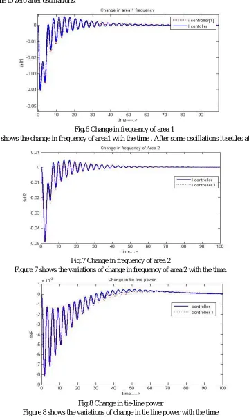
The change in frequency of area 1, area 2 and the change in tie line power graphs are observed. The simulation time is taken as 100.0s. The results come to zero after oscillations.

Fig.6 Change in frequency of area 1

Figure 6 shows the change in frequency of area1 with the time . After some oscillations it settles at zero.

Fig.7 Change in frequency of area 2

Figure 7 shows the variations of change in frequency of area 2 with the time.

Fig.8 Change in tie-line power

Technology (IJRASET)

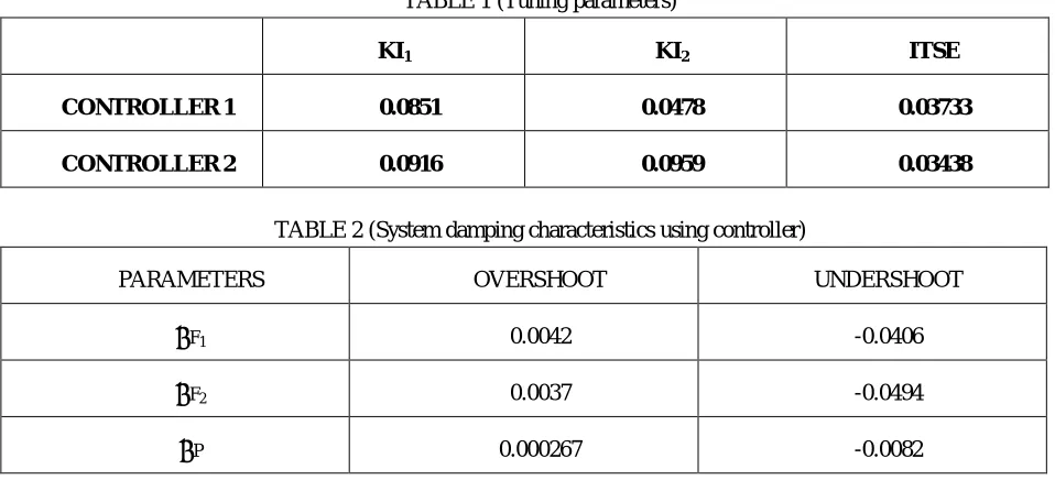
TABLE 1 (Tuning parameters)

KI1 KI2 ITSE

CONTROLLER1 0.0851 0.0478 0.03733

CONTROLLER2 0.0916 0.0959 0.03438

TABLE 2 (System damping characteristics using controller)

PARAMETERS OVERSHOOT UNDERSHOOT

ΔF1 0.0042 -0.0406

ΔF2 0.0037 -0.0494

ΔP 0.000267 -0.0082

VI. CONCLUSIONS

Controlling of power systems in order to meet the demands of consumers is a challenging task that motivates to design optimum controllers. They should have the capability of monitoring the power system like maintenance of frequency and voltage in no time. Many optimization techniques are used in the design of controllers. A two-area system is taken into consideration to show the method. The integral of time multiplied absolute error was used as objective function. Different plots of frequency deviation were obtained by varying the load demand of areas. Effects of parameter variation on system response were also plotted and observed. Its superiority over other methods used to tune the controller is justified by comparing the error values.

VII.ACKNOWLEDGMENT

I would like to thank Dr. (Prof.) Bibhu Prasad Panigrahi, Head of the Department, Electrical engineering at Indira Gandhi Institute of Technology, Sarang, and all the faculty members whose valuable guidance and encouragement to accomplish this job.

REFERENCES

[1] Mehrdad Tarafdar Hagh, Javad Morsali, “Effective oscillation damping of an interconnected multi-source power system with automatic generation control and TCSC”, Faculty of Electrical and Computer Engineering, University of Tabriz, Tabriz, Iran,Electrical Power and Energy Systems 65 (2015) 220–230. [2] M. Cengiz Taplamacioglu, Ilhan Kocaarslan, “Comparative performance analysis of Artificial Bee Colony algorithm in automatic generation control for

interconnected reheat thermal power system”, Gazi University, Faculty of Engineering, Department of Electrical & Electronics Engineering, Ankara, Turkey, Istanbul University, Faculty of Engineering, Department of Electrical & Electronics Engineering, Istanbul, Turkey,Electrical Power and Energy Systems 42 (2012) 167–178.

[3] Masoud Karimi-Ghartemani , Nasser Sadati, Mostafa Parniani, “Design of a fractional order PID controller for an AVR using particle swarm optimization”, Department of Electrical Engineering, University of California at Los Angeles, USA, Department of Electrical Engineering, Sharif University of Technology, Tehran, Iran, Control Engineering Practice 17 (2009) 1380–1387.

[4] Mohamed F. Hassan, Mohamed Zribi,” Decentralized load frequency controller for a multi-area interconnected power system”, Department of Electrical Engineering, Kuwait University, Kuwait, Electrical Power and Energy Systems 33 (2011) 198–209.

[5] Bibhu Prasad Ganthia, Smita Aparajita Pattanaik, Prashanta Kumar Rana, Samprati Mohanty “Compensation of Voltage Sag Using DVR with PI Controller” Department of Electrical and Electronics Engineering, DMI College of Engineering, Palanchur, Nazarethpet, Chennai, Tamil Nadu, India, IEEE Conference on International Conference on Electrical, Electronics, and Optimization Techniques (ICEEOT) – 2016, 3-5 March, 2016.