Formulation of a Model and Analysis of
Mechanical Timer Parameters by Using Response
Surface Method in MINITAB
Mayuri B.Ardak[1]Mr.M.R.Phate[2]
1,2
Mechanical Engineering Department, Pune University, Padmabhooshan Vasantadada Patil Institute of Technology Pune, India
Abstract :- Aim of this paper is to development methodology in MINITAB for design parameter analysis of mechanical timer unit which will give us required time delay, by forming mathematical model .Design parameters analysis was carried out in MINITAB using RSM to identify critical design parameters. It is effective to use the orthogonal arrays in fractional factorial designs. MINITAB offers four types of designed experiments: factorial, response surface, mixture, and Taguchi (robust). The steps follow in MINITAB to create, analyze, and graph an experimental design are similar for all design types. After conducting the experiment and enter the results, MINITAB provides several analytical and graphing tools to help to understand the results. While this paper demonstrates the typical steps for creating and analyzing a factorial design, These steps can be apply to any design which created in MINITAB to identify critical design parameters.
Keywords :- Response surface methodology, Orthogonal array, Taguchi Array, MINITAB
I. INTRODUCTION
In statistics, response surface methodology (RSM) explores the relationships between several explanatory variables and one or more response variables. The main idea of RSM is to use a sequence of designed experiments to obtain an optimal response. suggest using a second-degree polynomial model to do this. They acknowledge that this model is only an approximation, but use it because such a model is easy to estimate and apply, even when little is known about the process. An easy way to estimate a first-degree polynomial model is to use a factorial experiment or a fractional factorial design. This is sufficient to determine which explanatory variables have an impact on the response variable(s) of interest. Once it is suspected that only significant explanatory variables are left, then a more complicated design, such as a central composite design can be implemented to estimate a second-degree polynomial model, which is still only an approximation at best. However, the second-degree model can be used to optimize (maximize, minimize, or attain a specific target for).Practical concerns.Response surface methodology uses statistical models, and therefore practitioners need to be aware that even the best statistical model is an approximation to reality. In practice, both the models and the parameter
values are unknown, and subject to uncertainty on top of ignorance. Of course, an estimated optimum point need not be optimum in reality, because of the errors of the estimates and of the inadequacies of the model. Nonetheless, response surface methodology has an effective track-record of helping researchers improve products and services: For example, Box's original response-surface modelling enabled chemical engineers to improve a process that had been stuck at a saddle-point for years. The engineers had not been able to afford to fit a cubic three-level design to estimate a quadratic model, and their biased linear-models estimated the gradient to be zero. Box's design reduced the costs of experimentation so that a quadratic model could be fit, which led to a (long-sought) ascent direction.[1][2]
II EXPERIMENTAL
a) Identifying important parameters
From the literature and the previous work [6] done , among many independently controllable primary and secondary process parameters affecting the time delay, the primary process parameters viz Angle(A), Gear ratio(B), and Pallet weight (C) were selected as process parameters for this study. Angle(A), Gear ratio(B), and Pallet weight (C) are the primary parameters contributing to the required time delay
b) Orthogonal arrays Experiment
A lot of factors are often taken up at the same time at the early stage of the problem solving. The experiment frequency increases in the factorial experiment on which it experiments by all the level combinations when the number of factors taken up in the experiment increases. Then, the obtaining necessary information can be done by an experiment frequency that is less than the factorial experiment by providing experimental conditions by using the table that is called an orthogonal array. The experimental design is widely used in various fields including industry, medicine and psychology. The fractional factorial designs are effective when the number of factors considered is large and when it is difficult to experiment all the combinations. It is effective to use the orthogonal arrays in fractional factorial designs. The orthogonal arrays which will be used changes according to the number of factors and the number of levels considered. Two-level orthogonal arrays such as L8 and L16 are used when
factors of two levels are considered. Three-level orthogonal arrays such as L9and L27are used when factors of three levels
are considered. Their use and subsequent analysis are almost the same, but there is great difference in degrees of freedom.
In three-level orthogonal arrays, the degree of freedom a two factor interaction is four. Two factor interactions will appear across two columns. Due to this reason, the number of factors that can be considered is limited. Actually, there are only two prepared linear graphs for L27.
L27orthogonal array
In the factorial experiment, it is necessary to experiment by combining the levels of the factor taken up all. The total experiment frequency increases rapidly when the number of factors increases, and the inconvenience in the experiment is caused.. When the levels of all the factor taken up are three, the three-level orthogonal array is used.
C ) Development of mathematical model.
1. Response surface methodology
Response surface methodology(RSM) is a collection of mathematical and statistical technique useful for analyzing problems in which several independent variables influence a dependent variable or response and the goal is to optimize the response[14]. In many experimental conditions, it is possible to represent independent factors in quantitative form as given in Eq.(1). Then these factors can be thought of as having a functional relationship or response as follows:
Y=Φ(x1, x2, …,xk)±er (1)
Between the response Y and x1, x2, … ,xk of k quantitative factors, the function Φ is called response surface or response function. The residual er measures the experimental errors. For a given set of independent variables, a characteristic surface is responded. When the mathematical form of Φ is not known, it can be approximate satisfactorily within the experimental region by polynomial. In the present investigation, RSM has been applied for developing the mathematical model In applying the response surface methodology, the independent variable was viewed as a surface to which a mathematical model is fitted. The second order polynomial (regression) equation used to represent the response surface Y is given by[15]
Y = b0 +Σbi xi +Σbii xi +Σbij xi x j + e (2)
and for three factors, the selected polynomial could be expressed as
σ=b0+b1(N)+b2(S)+b3(F)+b11(N2)+b22(S2)+b33(F2)+
b12(NS)+b13(NF)+b23(SF) (3)
central composite face centred design surfaces very accurately
d) Formulation of Response Surface Model by MINITAB16 software
1.Response Surface Regression: T (Time) versus A (angle), B
(gear ratio), C (P Wt)
Before you use MINITAB, you need to determine what design is most appropriate for your experiment. Choosing your design correctly will ensure that the response surface is fit in the most efficient manner. MINITAB provides central composite and Box-Behnken designs. When choosing a design you need to identify the number of factors that are of interest. determine the number of runs you can perform ensure adequate coverage of the region of interest on the response surface. The next step is to fit the quadratic model. The quadratic model allows detection of curvature in the response surface.
The following terms cannot be estimated, and were removed. B (gear ratio)*C (P Wt)
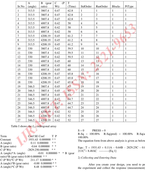
Table I shows the L27orthogonal array
Term Coef SE Coef T P Constant 1931.63 0.000000 * * A (angle) 0.11 0.000000 * * B (gear ratio) -0.64 0.000000 * * C (P Wt) -2829.250.000000 * *
A (angle)*A (angle) -0.01 0.000000 * * B (gear ratio)*B (gear ratio) 0.00 0.000000 * *
C (P Wt)*C (P Wt) 211.17 0.000000 * * A (angle)*B (gear ratio) -0.00 0.000000 * * A (angle)*C (P Wt) 8.48 0.000000 * *
S = 0 PRESS = 0
R-Sq = 100.00% R-Sq(pred) = 100.00% R-Sq(adj) = 100.00%
The equation form from above analysis is given as below, Equ.: T = 1931.63 + 0.11A – 0.64B – 2829.25C –0.01A2+ 211C2+ 8.48AC ---[Eq 1]
2) Collecting and Entering Data
After you create your design, you need to perform the experiment and collect the response (measurement) data. Sr.No
A (angle)
B (gear ratio)
C (P Wt)
T
To print a data collection form, follow the instructions below. After you collect the response data, enter the data in any worksheet column not used for the design.
Analysis of Variance for T (Time)
Source DF Seq SS Adj SS AdjMSF P Regression 8 410.447 410.447 51.3058 * *
Linear 3 310.821 37.877 12.6257 * * A (angle) 1 2.645 0.000 0.0002 * * B (gear ratio) 1 19.845 0.363 0.3629 * * C (P Wt) 1 288.331 1.217 1.2174 * * Square 3 13.519 37.184 12.3947 * *
A (angle)*A (angle) 1 13.202 13.202 13.2017 * *
B (gear ratio)*B (gear ratio) 1 0.202 0.868 0.8682 * *
C (P Wt)*C (P Wt) 1 0.116 0.001 0.0013 * * Interaction 2 86.107 86.107 43.0533 * *
A (angle)*B (gear ratio) 1 85.127 0.006 0.0056 * *
A (angle)*C (P Wt) 1 0.980 0.980 0.9797 * * Residual Error 18 0.000 0.000 0.0000
Pure Error 18 0.000 0.000 0.0000 Total 26 410.447
ObsStdOrder T (Time) Fit SE Fit Residual Resid 1 1 62.800 62.800 0.000 0.000 * 2 2 62.800 62.800 0.000 0.000 * 3 3 62.800 62.800 0.000 0.000 * 4 4 58.000 58.000 0.000 0.000 * 5 5 58.000 58.000 0.000 0.000 * 6 6 58.000 58.000 0.000 0.000 * 7 7 61.200 61.200 0.000 0.000 * 8 8 61.200 61.200 0.000 0.000 * 9 9 61.200 61.200 0.000 0.000 * 10 10 59.500 59.500 0.000 -0.000 * 11 11 59.500 59.500 0.000 -0.000 * 12 12 59.500 59.500 0.000 -0.000 * 13 13 60.000 60.000 0.000 0.000 * 14 14 60.000 60.000 0.000 0.000 * 15 15 60.000 60.000 0.000 0.000 * 16 16 65.800 65.800 0.000 0.000 * 17 17 65.800 65.800 0.000 0.000 * 18 18 65.800 65.800 0.000 0.000 * 19 19 63.000 63.000 0.000 0.000 * 20 20 63.000 63.000 0.000 0.000 * 21 21 63.000 63.000 0.000 0.000 * 22 22 64.700 64.700 0.000 -0.000 *
23 23 64.700 64.700 0.000 -0.000 * 24 24 64.700 64.700 0.000 -0.000 * 25 25 52.000 52.000 0.000 0.000 * 26 26 52.000 52.000 0.000 0.000 * 27 27 52.000 52.000 0.000 0.000 *
Predicted Response for New Design Points Using Model for T (Time)
SE
Point Fit Fit 95% CI 95% PI 1 62.8 0 (62.8, 62.8) (62.8, 62.8) 2 62.8 0 (62.8, 62.8) (62.8, 62.8) 3 62.8 0 (62.8, 62.8) (62.8, 62.8) 4 58.0 0 (58.0, 58.0) (58.0, 58.0) 5 58.0 0 (58.0, 58.0) (58.0, 58.0) 6 58.0 0 (58.0, 58.0) (58.0, 58.0) 7 61.2 0 (61.2, 61.2) (61.2, 61.2) 8 61.2 0 (61.2, 61.2) (61.2, 61.2) 9 61.2 0 (61.2, 61.2) (61.2, 61.2) 10 59.5 0 (59.5, 59.5) (59.5, 59.5) 11 59.5 0 (59.5, 59.5) (59.5, 59.5) 12 59.5 0 (59.5, 59.5) (59.5, 59.5) 13 60.0 0 (60.0, 60.0) (60.0, 60.0) 14 60.0 0 (60.0, 60.0) (60.0, 60.0) 15 60.0 0 (60.0, 60.0) (60.0, 60.0) 16 65.8 0 (65.8, 65.8) (65.8, 65.8) 17 65.8 0 (65.8, 65.8) (65.8, 65.8) 18 65.8 0 (65.8, 65.8) (65.8, 65.8) 19 63.0 0 (63.0, 63.0) (63.0, 63.0) 20 63.0 0 (63.0, 63.0) (63.0, 63.0) 21 63.0 0 (63.0, 63.0) (63.0, 63.0) 22 64.7 0 (64.7, 64.7) (64.7, 64.7) 23 64.7 0 (64.7, 64.7) (64.7, 64.7) 24 64.7 0 (64.7, 64.7) (64.7, 64.7) 25 52.0 0 (52.0, 52.0) (52.0, 52.0) 26 52.0 0 (52.0, 52.0) (52.0, 52.0)
27 52.0 0 (52.0, 52.0) (52.0, 52.0)
III. GRAPH WINDOW OUTPUT
b) Plotting the Response Surface.
You can use Contour/Surface (Wireframe) Plots to display two types of response surface plots: contour plots and surface plots (also called wireframe). These plots show how are response variable relates to two factors based on a model equation .Contour and surface plots are useful for establishing desirable response values and operating conditions. In a contour plot, the response surface is viewed as a two-dimensional plane where all points that have the same response are connected to produce contour lines of constant responses surface plot displays a three-dimensional view that may provide a clearer picture of the response surface. The illustrations below compare these two types of plots.
C) Contour Plot.
d) Surface Plot
IV. OPTIMIZATION OF MODEL
a) Optimising parameters
Contour plots show distinctive circular shape indicative of possible independence of factors with response. A contour plot is produced to visually display the region of optimal factor settings. For second order response surfaces, such a plot can be more complex than the simple series of parallel lines that can occur with first order models. Once the stationary point is found, it is usually necessary to characterize the response surface in the immediate vicinity of the point by identifying whether the stationary point found is a maximum response or minimum response or a saddle point. To classify this, the most straightforward way is to examine through a contour plot. Contour plots play a very important role in the study of the response surface. By generating contour plots using software for response surface analysis, the optimum is located with reasonable accuracy by characterizing the shape of the surface. If a contour patterning of circular shaped contours occurs, it tends to suggest independence of factor effects while elliptical contours as may indicate factor interactions.
Response surfaces have been developed for both the models, taking two parameters in the middle level and two parameters in the X and Y axis and response in Z axis. The response surfaces clearly reveal the optimal response point. RSM is used to find the optimal set of process parameters that produce a maximum or minimum value of the response. In the present investigation the process parameters corresponding to the maximum tensile strength are considered as optimum (analyzing the contour graphs and by solving Eq.(4)). Hence, when these optimized process parameters are used, then it will be possible to attain the maximum tensile strength.
6.0000E-13 4.0000E-13 2.0000E-13 0.0000E+00 -2.000E-13 99 90 50 10 1
Residual 50 55 60 65
4.0000E-13 2.0000E-13 0.0000E+00 -2.000E-13 Fitted Value 8 6 4 2 0 Residual 26 24 22 20 18 16 14 12 10 8 6 4 2 4.0000E-13 2.0000E-13 0.0000E+00 -2.000E-13 Observation Order
Normal Probability Plot Versus Fits
Histogram Versus Order
Residual Plots for T (Time)
B (gear ratio)*A (angle)
340 330 320 4200 4100 4000 3900
C (P Wt)*A (angle)
340 330 320 0.468 0.456 0.444 0.432 0.420
C (P Wt)*B (gear ratio)
4200 4100 4000 3900 0.468 0.456 0.444 0.432 0.420
A (angle) 330 B (gear ratio) 4008 C (P Wt) 0.445
Hold Values > – – – – – – < 50.0 50.0 52.5 52.5 55.0 55.0 57.5 57.5 60.0 60.0 62.5 62.5 65.0 65.0 T (Time) Contour Plots of T (Time)
58 60 62
320330 340 320330 62 64 3800 340 4000 3800 4200 4000 T (Time)
B (gear ratio) A (angle)
50 55 60
320 330340 320 330 60 65 0.42 340 0.46 0.44 0.42 0.46 T (Time)
C (P Wt) A (angle)
55 60
3800 3800 4000 3800 40004000 65 0.42 4200 0.46 0.44 0.42 0.46 0.44 T (Time)
C (P Wt) B (gear ratio)
A (angle) 330 B (gear ratio) 4008 C (P Wt) 0.445
Hold Values
b) Response Optimization
Parameters Goal Lower Target Upper Weight Import T (Time) Target 59 60 61 1 1
Global Solution A (angle) = 313.5 B (gear rati = 4180.91 C (P Wt) = 0.42 Predicted Responses
T (Time) = 60, desirability = 1.000000 Composite Desirability = 1.000000
C) Optimization Plot
Main Effects Plot
The same steps are followed for another six design parameters in two sets. The other two equations and main effects plot for these two sets of parameters are given below.
Readings for Other Two Sets Parameter Set 2:
A: Pallet Radius B: Pin Radius
C: Escarpment Wheel Radius
The equation form for above parameter is given below
T = -69.6938 + 21.6833A + 20.6667B + 11.240C –1.283A2+ 66.6667B2–0.7167C2–3.1667AB
Main effects plot for these parameters is give below,
Cur
High Low 1.0000D Optimal
d = 1.0000 Targ: 60.0T (Time)
y = 60.0
1.0000 Desirability Composite
0.420 0.4700 3807.40
4208.1900 313.50
346.50 B (gear C (P Wt)
A (angle
[313.50] [4180.9100] [0.420]
346.5 330.0 313.5 64
62
60
58
56
4208.19 4007.80 3807.40
0.47 0.45 0.42 64
62
60
58
56
A (angle) B (gear ratio)
C (P Wt)
Main Effects Plot for T (Time)
Data Means
7 6 5 65
60
55
0.3 0.2 0.1
8.04 7.04 6.04 65
60
55
A (Pallet Radi) B (Pin Radi)
C (Esc. W heel Radi)
Main Effects Plot for T (Time)
Parameter Set 3: A: Pallet to pin distance
B: Distance between pallet and escapement wheel C: Tooth angle for escapement wheel
The equation form for above parameter is given below
T = 1638.62 + 8.45A + 4.12B –48.87C –0.02A2–0.07B2+ 0.37C2- 0.43AB
Main effects plot for these parameters is give below,
V) RESULT &
CONCLUSION:-The response surface methodology analysis has been reviewed. RSM can be used for the approximation of both experimental and numerical responses. Two steps are necessary, the definition of an approximation function and the design of the plan of experiments .From the experimentation we got the global value (60 min) of time by using various parameters i.e. angle, gear ratio, pallet weight, pallet radius, pin radius, escarpment wheel radius, pallet to pin distance, distance between pallet and escapement wheel and tooth angle for escapement wheel. The most effecting parameter are find out from the main effects plots for all nine parameters against Time ( T ).
The main effecting parameters are as follows, A:Pallet weight
B: Pallet radius C: Pin Radius D: Pin Dist.
In above parameters pallet weight and pallet radius are directly proportional to each other, hence we consider next parameter for our further design study. Those parameters are
A:Pallet weight, B: Pin Radius and C: Pin Dist. VI) References
[1] G.E.P. Box and D.W. Behnken (1960). “SOME NEW THREE LEVEL DESIGNS FOR THE STUDYOF
QUANTITATIVE VARIABLES,” Technometrics 2, pp.455–
475.
[2] G.E.P. Box and N.R. Draper (1987). EMPIRICAL
MODEL-BUILDING AND RESPONSE SURFACES,John
Wiley & Sons.p.249.
[3] A.I. Khuri and J.A. Cornell (1987).RESPONSE
SURFACES: DESIGNS AND ANALYSES, Marcel
Dekker, Inc.
[4] D.C. Montgomery (1991). DESIGN AND ANALYSIS OF
EXPERIMENTS, Third Edition, John.Wiley & Sons.
[5]Syuhei Okada1, Yasuhiro Itoh2, Tomomichi Suzuki31”EXPERIMENTALDESIGN TO ALLOCATE MORE FACTORS TO L27,”12, 3Department of Industrial
Administration, Tokyo University of Science2641 Yamazaki, Noda, Chiba, 278-8510, JAPAN
[6]Mayuri Ardak,M.R.Phate “MATHEMATICAL
MODELING AND COMPUTER SIMULATION FOR MECHANICAL TIMER RUNWAY ESCAPEMENT
MECHANISM” published in International Journal of Science,
Engineering and Technology Research (IJSETR) Volume 3, Issue 5, May 2014
5.34 4.34
3.34 65.0
62.5
60.0
57.5
55.0
8.58 7.58 6.58
67.5 66.5
65.5 65.0
62.5
60.0
57.5
55.0
A (pin Dist .) B (Pallet and Esc. Dist )
C (Esc.T ooth Angle)
Main Effects Plot for T (Time)