Tensorial blind source separation for improved analysis of multi omic data

M E T H O D

Open Access

Tensorial blind source separation for

improved analysis of multi-omic data

Andrew E. Teschendorff

, Han Jing

, Dirk S. Paul

, Joni Virta

and Klaus Nordhausen

Abstract

There is an increased need for integrative analyses of multi-omic data. We present and benchmark a novel tensorial independent component analysis (tICA) algorithm against current state-of-the-art methods. We find that tICA outperforms competing methods in identifying biological sources of data variation at a reduced computational cost. On epigenetic data, tICA can identify methylation quantitative trait loci at high sensitivity. In the cancer context, tICA identifies gene modules whose expression variation across tumours is driven by copy-number or DNA methylation changes, but whose deregulation relative to normal tissue is independent of such alterations, a result we validate by direct analysis of individual data types.

Keywords: Multi-omic, Tensor, Dimensional reduction, Independent component analysis, mQTL, Epigenome-wide association study, Cancer

Background

Omic data is now most often generated in a multi-dimensional context. For instance, for the same individual and tissue type, one may measure different data modali-ties (e.g. genotype, mutations, DNA methylation or gene expression), which may help pinpoint disease-driver genes [1]. Alternatively, for the same individual, the same data type may be measured across different tissues or cell types [2, 3], which may help identify the most relevant cell types or tissues for understanding disease aetiology. We refer to all of these types of multi-dimensional data generally as multi-way or multi-omic data, and when sam-ples and molecular features are matched, the data can be brought into the form of a multi-dimensional array, formally known as a tensor [4].

While several statistical algorithms for the analysis of multi-way or tensorial data are available [4–7], their appli-cation to real data has been challenging. There are mainly three reasons for this. First, the associated multi-way

*Correspondence:[email protected]

†_{Andrew E. Teschendorff and Han Jing contributed equally to this work}

1_{CAS-MPG Partner Institute for Computational Biology, CAS Key Lab of}

Computational Biology, Shanghai Institute for Biological Sciences, Chinese Academy of Sciences, 320 Yue Yang Road, 200031 Shanghai, China

2_{Department of Women’s Cancer, UCL Elizabeth Garrett Anderson Institute for}

Women’s Health, University College London, 74 Huntley Street, WC1E 6BT London, UK

Full list of author information is available at the end of the article

datasets are often very large and how well the algorithms perform on such large sets is currently still unclear. Sec-ond, the algorithms can be computationally demanding, compromising their benefit-to-cost ratio [4]. Third, inter-preting the output of these algorithms requires an in-depth understanding of the underlying methods. Exac-erbating this problem, most available software packages are not user-friendly, requiring the user to have such an in-depth understanding to extract the relevant biological information. Beyond these technical challenges, there is also a lack of comparative studies, making it difficult to choose the appropriate algorithm for the task in question. To help address some of these outstanding challenges, we here consider and evaluate a novel data tensor decom-position algorithm [8,9], which is based on blind source separation (BSS), and specifically independent compo-nent analysis (ICA) [10]. Although common BSS tech-niques such as non-negative matrix factorisation and ICA have been successfully applied to a wide range of single omic data types, including e.g. gene expression [11–16], DNA methylation [17] and mutational data [18], their application to multi-way data is largely unexplored [19]. For single-omic datasets, the improved performance of ICA over non-BSS techniques like principal compo-nent analysis (PCA) is due primarily to the non-Gaussian and often sparse nature of biological sources of variation, which means that statistical deconvolution of biological

samples benefits from non-linear decorrelation measures such as statistical independence (as used in ICA) [13]. It is, therefore, natural to consider analogous ICA algorithms for multi-way data, as we do here, since these may also lead to improved inference.

To assess this, we here benchmark our novel tensorial BSS algorithm against some of the most popular and pow-erful algorithms for inferring sources of variation from multi-omic data, including JIVE (joint and individual vari-ation explained) [5], PARAFAC (parallel factor analysis) [4, 6], iCluster [7] and canonical correlation analysis (CCA) [20–22]. Each of these algorithms has particu-lar strengths and weaknesses, which render comparisons between them highly non-trivial. For instance, a limitation of CCA is that it can infer only common sources of vari-ation between data types or tissues, in contrast to JIVE or PARAFAC, which can infer both joint as well as indi-vidual sources of variation. On the other hand, JIVE and CCA can be run on multiple data matrices with differ-ent numbers of molecular features, while PARAFAC and iCluster require matched sets of features (and samples) for each data type. Model complexity also differs sub-stantially between methods, with PARAFAC exhibiting a much lower model complexity than an algorithm such as iCluster. Thus, a comparison of all of these methods is of paramount interest, and here we do so in a tensorial con-text, i.e. one where the multi-way data is defined over a matched set of molecular features (e.g. genes or CpGs) and samples across all data types, allowing the data to be brought into the form of a tensor. Specifically, we shall here consider order-3 data tensors, i.e. data which can be brought into the form of an array with three dimensions (often called modes). In our evaluation and comparison of all multi-way algorithms, we consider both simulated data as well as data from real epigenome-wide associa-tion studies (EWAS). We further illustrate potential uses of our tensorial BSS algorithm (i) to detect cell-type-independent and cell-type-specific methylation quantita-tive trait loci (mQTLs) in multi-cell-type or multi-tissue EWAS and (ii) to detect cancer gene modules deregulated by copy-number and DNA methylation changes.

Results

Tensorial ICA outperforms JIVE, PARAFAC, iCluster and CCA on simulated data

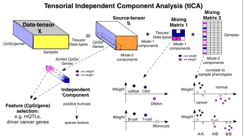
Tensorial ICA (tICA) aims to infer from a data tensor statistically independent sources of data variation, which should correspond better to underlying biological factors (‘Methods’). Indeed, since biological sources of data vari-ation are generally non-Gaussian and often sparse, the statistical independence assumption implicit in the ICA formalism can help improve the deconvolution of com-plex mixtures and thus, better identify the true sources of data variation (Fig.1). As with ordinary ICA itself, there

are different ways of implementing tICA, and we here consider two different flavours: tensorial fourth-order blind identification (tFOBI) and tensorial joint approxi-mate diagonalisation of high-order eigenmatrices (tJADE) (‘Methods’). Specifically, we consider two modified ver-sions of these, whereby tensorial PCA is applied as a noise reduction step (also called whitening) prior to implement-ing tICA, resultimplement-ing in two algorithms we call tWFOBI and tWJADE (‘Methods’).

Data-tensor

X

=

_*

Source-tensor

S

*

Mixing Matrix 2

Tensorial Independent Component Analysis (tICA)

CpGs/genes

Samples

Tissues/

Data-types CpGs/ Genes

Mode-2 components

Mode-1 components

Samples

Mode-1 components

Mode-2 components

Independent Component

Feature (CpG/gene) selection: e.g. mQTLs, driver cancer genes

Tissues/ Data-types

+ve weight -ve weight

cancer

normal

Weight

correlate to sample phenotypes

A/A A/B

Weight

B/B

Weight _{mRNA CNV}

DNAm

Weight

B-cell T-cell

Monocyte

+ve weight -ve weight Sorted CpGs/

Genes

positive kurtosis

sparse factors

Fig. 1Decomposing data tensors using independent component analysis. Tensorial ICA (tICA) works by decomposing a data tensor, here depicted as an order-3 tensor with three dimensions representing features (CpGs/genes), samples and tissue or data type, into a source tensorSand two mixing matrices defined over tissue/data type and samples, respectively. The key property of tICA is that the independent components inSare as statistically independent from each other as possible. Statistical independence is a stronger criterion than linear decorrelation and allows improved inference of sparse sources of data variation. Positive kurtosis can be used to rank independent components to select the most sparse factors. The largest absolute weights within each independent component can be used for feature selection, while the corresponding component in the mixing matrices informs about the pattern of variation of this component across tissue/data types and samples, respectively. In the latter case, the weights can be correlated to sample phenotypes, such as normal/cancer status or genotype. For the first mixing matrix, the weights inform us about the relation between data types (e.g. if the copy-number change is positively correlated with gene expression), or for a multi-cell EWAS, whether mQTLs are cell type independent or not.+ve positive,−ve negative, CNV copy-number variation, DNAm DNA methylation, EWAS epigenome-wide association study, mQTL methylation quantitative trait locus, mRNA messenger RNA

indicating that our results are not dependent on the type of data distribution (Additional file1: Figure S1).

Tensorial PCA/ICA reduces running time compared to JIVE, PARAFAC and iCluster

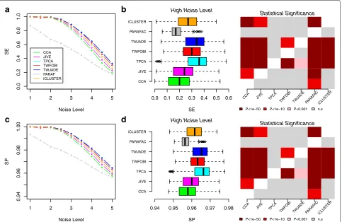
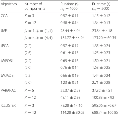
Using the same simulated data, we further compared the algorithms in terms of their running times. A detailed comparison is cumbersome because the param-eters specifying the number of components to search for are not directly comparable and differ substantially between methods. Nevertheless, using reasonable param-eter choices for the simulated model above, we found that tPCA and tICA substantially speed up inference over methods such as JIVE or iCluster (Table1). In fact, even when specifying a larger number of components for tPCA/tICA, compared to PARAFAC, JIVE or iCluster, the latter were substantially slower (Table1), whilst also exhibiting marginally worse SE and SP values (Fig.2). In general, we observed tICA methods to be at least 50 times

faster than PARAFAC, and at least 100 times faster than JIVE and iCluster (Table1). For much larger datasets, we found the application of iCluster to be computationally demanding and not practical. Thus, in subsequent analy-ses on real datasets, we decided to benchmark tPCA/tICA against PARAFAC, CCA, SCCA and JIVE.

tICA exhibits improved power in a real multi-tissue smoking EWAS

1 2 3 4 5

0.0

0.2

0.4

0.6

0.8

1.0

Noise Level

SE

a

CCA JIVE TPCA TWFOBI TWJADE PARAF iCLUSTER

1 2 3 4 5

0.94

0.96

0.98

1.00

Noise Level

SP

c

SE

b

0.0 0.1 0.2 0.3 0.4 0.5 0.6

CCA JIVE TPCA TWFOBI TWJADE PARAFAC iCLUSTER

SP

d

0.94 0.95 0.96 0.97 0.98

CCA JIVE TPCA TWFOBI TWJADE PARAFAC iCLUSTER

Statistical Significance

CCA JIVE TPCA TWFOBI TW

JADE PARAF

AC

iCLUSTER

P<1e−50 P<1e−10 P<0.001 n.s

Statistical Significance

CCA JIVE TPCA TWFOBI TWJ

ADE PARAF

AC

iCLUSTER

P<1e−50 P<1e−10 P<0.001 n.s

Fig. 2Comparison of multi-way algorithms on simulated data.aSensitivity (SE) versus noise level (x-axis) for seven different methods as indicated, as evaluated on simulated data (data points are averages over 1000 Monte Carlo runs). In each case, the data tensor was of size 2×100×1000, i.e. two data types, 100 samples and 1000 genes.bLeft panel: Box plots of SE values for the same seven methods for the largest noise level (5). Each box contains the SE values over the 1000 Monte Carlo runs. Right panel: Corresponding heat map ofPvalues of significance for each pairwise

comparison of methods.Pvalues were computed from a one-tailed Wilcoxon rank sum test. For each entry specified by a given row and column, the alternative hypothesis is that the method specified in the row has a higher SE than the method specified in the column.c,dAsa,b, but for the specificity (SP). SE sensitivity, SP specificity

DNA methylation (DNAm) is measured in buccal samples [2]. Thus, one way to compare algorithms objectively is in terms of their sensitivity to identify these 62 smkDMCs in a matched blood-buccal EWAS consisting of Illu-mina 450k DNAm profiles for a total of 152 women (‘Methods’, [2]). Because there are two distinct samples (one blood plus one buccal) per individual, most of the variation is genetic. Hence, to reduce this background genetic variation, we first computed the SE values on a reduced data matrix obtained by combining the 62 smkDMCs with 1000 randomly selected non-smoking associated CpGs (a total of 100 Monte Carlo randomi-sations). We considered both the maximum SE value attained by a component, as well as the overall SE obtained by combining selected CpGs from components signifi-cantly enriched for smkDMCs (‘Methods’). This revealed that JIVE, CCA/SCCA and PARAFAC were all superseded by tPCA and tICA (Fig.3a,b). Differences between tPCA and tICA were generally not significant (Fig.3a), although

tWFOBI attained higher combined SE values than tPCA and tWJADE (Fig.3b).

Next, we scaled up the data matrices by combining the 62 smkDMCs with a larger set of 10 000 non-smkDMCs, recomputing the SEs (again for 100 different Monte Carlo selections of 10 000 non-smkDMCs). As expected, with an increase in the number of CpGs, the SE of all algo-rithms dropped, likely driven by increased confounding due to genetic variation (Fig. 3c,d). With the increase in probe number, tICA (tWFOBI and tWJADE) outper-formed not only JIVE, PARAFAC and CCA/SCCA, but also tPCA (Fig.3c,d), in line with the increased sparsity of the smoking-associated source of variation.

Table 1Comparison of running times of multi-way algorithms

Algorithm Number of Runtime (s) Runtime (s) components ng=1000 ng=2000

CCA K₌3 0.57_±0.11 1.15_±0.12

K₌12 0.58_±0.14 1.34_±0.13

JIVE jV=1,iV=(1, 1) 28.44±4.04 23.84±4.18 jV=4,iV=(4, 4) 137.77±44.94 173.20±60.35

tPCA (2,2) 0.57±0.17 1.35±0.24

(2,6) 0.61±0.15 1.25±0.23

tWFOBI (2,2) 0.65±0.16 1.50±0.21

(2,6) 0.76±0.14 1.53±0.25

tWJADE (2,2) 0.66±0.19 1.44±0.24

(2,6) 1.23±0.21 2.71±0.28

PARAFAC R=6 22.37±2.53 37.32±4.51

R=12 48.11±2.98 100.83±7.92

iCLUSTER K=3 79.28±14.16 595.06±70.67

K₌12 114.28_±30.02 688.74_±166.85

Seven multi-way algorithms in terms of the running times to infer components of variation (runtime) in the simulation model considered in Fig.2. Estimates are medians and median absolute deviations over 100 Monte Carlo runs for when the signal-to-noise ratio is 1 (i.e. noise level = 3 in Fig.2). The second column specifies the parameter values for the number of components used in each algorithm. The first rows for each method are as follows. For CCA, three sets of canonical vector pairs (K=3) are shown. For JIVE, the rank of joint variation (jV=1) and rank of individual variation (iV=1) for each data type are shown. For TPCA, TWFOBI and TWJADE, we inferred two components for both the data type and sample dimensions. For PARAFAC, the rank of decomposition wasR=6 and for iCLUSTER the maximum number of clustersKwas set to 3. For the second rows, the total number of components is exactly matched (12) for all methods. The running times are reported for two scenarios differing in the number of genesng, as indicated, and were obtained on a Dell PowerEdge R830 with Intel Xeon E5-4660 v4 2.2 GHz processors

a less correlative structure than the corresponding com-ponents projected onto the blood and buccal dimensions, demonstrating that tWJADE does indeed identify compo-nents that are less statistically dependent (Fig.4a). Con-firming the high sensitivity of these ICs, the 62 smkDMCs were highly enriched among CpGs with the largest abso-lute weights in any one of the two ICs (Fig. 4a, Fisher testP < 1×10−36 _{and SE = 41/62 ∼ 0.66). We}

fur-ther verified that the 41 enriched smkDMCs exhibited strong Pearson correlations between their DNAm profiles in blood and buccal, as required since smoking exposure is associated with similar DNAm patterns in these two tis-sue types (Fig.4b) [2]. Further confirming that component 12 is associated with smoking exposure, we correlated the weights of the corresponding column of the estimated mixing matrix with two different measures of smoking exposure, demonstrating in both cases a strong associa-tion (Fig.4c). Thus, application of tICA on DNAm data results in components that are readily interpretable in terms of their associations with known smoking exposure across features and samples.

tICA identifies mQTLs in a multi-cell-type EWAS

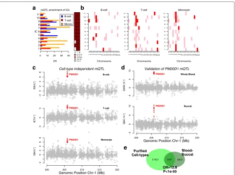
Having established the better performance of tICA over other state-of-the-art methods, we next considered the application of tICA (specifically tWFOBI) in an EWAS of 47 healthy individuals, for which three purified cell types (B cells, T cells and monocytes) have been profiled with Illumina 450k DNAm bead arrays [3] (‘Methods’). We chose tWFOBI over tWJADE because of its compu-tational efficiency (Table 1). Given that three cell types were measured for each individual, the expectation is that a significant amount of inter-individual variation in DNAm would correlate with genetic variants (i.e. mQTLs) [24]. Thus, it is important to evaluate the ability of tICA to detect mQTLs and to determine whether these are blood-cell-subtype specific or not. Applying tWFOBI to the data tensor for the 3 cell types × 47 samples×388 618 probes, we inferred a total of 11 ICs in the sample-mode space (yielding 33 ICs across sample and cell-type modes combined). For each of these 11 ICs in each cell type, we ranked probes according to their absolute weights and tested the enrichment of the top-500 probes against a high-quality list of 22 245 mQTLs as derived in [25] (‘Methods’). This high-confidence list of mQTLs all passed a very stringent unadjusted P

value threshold of P = 1 × 10−14 in each of five dif-ferent human cohorts, encompassing five difdif-ferent age groups [25]. We observed strong statistical enrichment for mQTLs in many ICs (Fig. 5a). We also tested sep-arately for enrichment of chromosomes. This revealed enrichment, notably of chromosomes 6 and 21, but also of 1, 4, 7 and 8 (Fig.5b). For instance, IC-9 was enriched for mQTLs and chromosome 1 in all three cell types (Fig. 5a,b). Supporting this, we found a clear example of a cell-type-independent mQTL mapping to the 1q32 locus of thePM20D1gene (Fig.5c), a major genome-wide association study (GWAS) locus associated with Parkin-son’s disease [26]. Focusing on chromosome 6, another cell-type-independent mQTL mapped to MDGA1

(Additional file 1: Figure S2), a major susceptibility locus for schizophrenia [27]. Other mQTLs driving ICs were cell type specific, e.g. mQTLs mapping to

ATXN1 andSYNJ2were dominant in the ICs projected

SE(Max) 0.0 0.2 0.4 0.6 0.8 1.0 CCA

SCCA JIVE tPCA tWFOBI tWJADE PARAFAC

a

CCA _SCCA JIVE tPCA tWFOBI tWJ

ADE PARA

FAC

P<1e−50 P<1e−10 P<0.001 n.s _SE(All) 0.0 0.2 0.4 0.6 0.8 1.0 CCA

SCCA JIVE tPCA tWFOBI tWJADE PARAFAC

b

CCA _SCCA JIVE tPCA tWFOBI tWJ

ADE PARAF

AC

P<1e−50 P<1e−10 P<0.001 n.s

SE(Max) 0.0 0.1 0.2 0.3 0.4 0.5 CCA

SCCA JIVE tPCA tWFOBI tWJADE PARAFAC

c

CCA _SCCA JIVE tPCA tWFOBI tWJ

ADE PARA

FAC

P<1e−50 P<1e−10 P<0.001 n.s SE(All) 0.0 0.1 0.2 0.3 0.4 0.5 CCA

SCCA JIVE tPCA tWFOBI tWJADE PARAFAC

d

CCA _SCCA JIVE tPCA tWFOBI tWJ

ADE PARAF

AC

P<1e−50 P<1e−10 P<0.001 n.s

Fig. 3Comparison of multi-way algorithms on a multi-tissue smoking EWAS.aLeft panel: Box plot of sensitivity (SE) values for each of the seven methods as applied to the data tensors of dimension 2_×152_×1062 (two tissues, 152 samples and 1000 randomly selected non-smkDMCs plus 62 smkDMCs) and for 100 different selections of non-smkDMCs. SE(Max) is the maximum sensitivity to capture 62 smkDMCs among all inferred components. Right panel: Heat map of the corresponding one-tailed paired Wilcoxon rank sum test, benchmarking the SE values of each method (y-axis) against each other method (x-axis).bAsa, but now for the combined sensitivity (SE(All)) obtained from all enriched components.c,dAsa,b, but now for data tensors of dimension 2_×152_×10 062 and for 100 randomly selected 10 000 non-smkDMCs. EWAS epigenome-wide association study, SE sensitivity, smkDMC smoking-associated differentially methylated CpG, SP specificity

Next, we validated the mQTLs found using an inde-pendent dataset. Thus, we applied tWFOBI to the blood-buccal EWAS considered earlier. We inferred a source tensor of dimension 2×26× 447 259, i.e. a total of 52 ICs, defined over two tissue types and 26 components in sample-mode space. As before, we observed very strong enrichment, notably for the same chromosomes 6 and 21 (Additional file1: Figure S5). The previously found mQTL at the PM20D1 locus was also prominent in one of the inferred ICs in this blood-buccal EWAS, confirming its validity and further supporting that this mQTL is cell type independent (Fig.5d). Overall, from the pure blood-cell-subtype EWAS, we detected a total of 1763 mQTLs, of which 547 were also observed in the blood-buccal EWAS (odd ratio = 12.8, Fisher test P < 1× 10−50, Fig. 5e). Thus, we can conclude that tWFOBI is able to identify components of variation across cell types and samples that capture a significant number of mQTLs, without matched genotype information.

tICA outperforms JIVE and PARAFAC in their sensitivity to detect mQTLs

−6 −4 −2 0 2 4 6 8

−15

−10

−5

0

5

10

S[1,12,]

S[2,12,]

a

smkDMC Random

−40 −20 0 20 40

−40

−20

0

20

S[WB,12,]

S[B

UC

,12,]

smkDMC Random

0 2 4 6 8

0

5

10

15

|S[1,12,]|

|S[2,12,]|

Fisher test P<1e−36

b

Enriched smkDMCs(WB)

Enr

iched smkDMCs (B

UC)

Correlations: WB with BUC

−1 0.4 0.4 1

0 10 20 30 40

−2

02

4

SmokingPackYears

Mix[,12]

c

P=8e−11

Never ExSmk Smoker

−2

0

2

4

P=1e−12

Fig. 4Validation of tensorial ICA on multi-tissue smoking EWAS.aLeft panel: Scatterplot of the weights of estimated independent components

S1,12,iandS2,12,ifrom the data tensor of dimension 2×152×1062, with mode 1 representing tissue type, mode 2 the different women and mode 3

the CpGs. Red denotes the smkDMCs. Middle panel: As left panel, but now for the rotated tensor, projecting the data onto the whole blood (WB) and buccal (BUC) dimensions, demonstrating the strong correlation between the DNAm variation in whole blood and buccal tissue. Right panel: As left panel, but now for the absolute weights. The green dashed lines represent the cutoff point selecting the 62 CpGs with the largest absolute weights. There are in total 41 smkDMCs among the three larger quadrants, corresponding to a sensitivity of 41/62=0.66, with the enrichmentP

value given above the plot.bPearson correlation heat map of the 41 smkDMCs between whole blood (WB) and buccal (BUC) tissue, with correlations computed over the 152 samples.cPlots of the 12th independent component of the mixing matrix in the sample space (y-axis) against smoking exposure for the 152 samples. Left panel: Smoking-pack-years. Right panel: Smoking status (never smokers, ex-smokers and smokers at sample draw).Pvalues are from linear regressions. BUC buccal, DNAm DNA methylation, EWAS epigenome-wide association study, ExSmk ex-smoker, smkDMC smoking-associated differentially methylated CpG, WB whole blood

for the tICA methods (Fig. 6b). To better evaluate the enrichment of these components for mQTLs, we also con-sidered the ratio of the sensitivity to the maximum possi-ble sensitivity, recording the maximum value attained by any component. This demonstrated that when selecting the top-500 CpGs, the components inferred using tICA could capture over 60% of the maximum possible num-ber of mQTLs, i.e. over 60% of the 500 CpGs mapped to mQTLs (Fig.6c). In contrast, JIVE components con-tained only just over 40% of mQTLs (Fig.6c). We note that although the performance of JIVE could be significantly improved by also including the components of individual variation, that approximately 80% of mQTLs have been estimated to be independent of blood cell subtype [28], supporting the view that JIVE is less sensitive in capturing

cell-type-independent mQTLs. All these results were sta-ble to repeated runs of the algorithms, as only PARAFAC exhibited variation between runs. However, this variation was relatively small (Additional file1: Figure S6).

OR 0 10 20 30 40 1 2 3 4 5 6 7 8 9 10 11 IC

a

B T M

P<1e-10 P<1e-5 P<0.001 P<0.05 P=n.s Chromosome 1 2 3 4 5 6 7 8 9 10 11

123456789

10111213141516171819202122

B-cell

b

123456789

1

0

1

1

1213141516171819202122

T-cell Chromosome 1 2 3 4 5 6 7 8 9 10 11

123456789

10111213141516171819202122

Monocyte S [B ,9,*] -2 0 2468

Cell-type independent mQTL

B-cell

c

5 PM20D1 T-cell

S[M ,9, *] -4 0 2 4 68 Monocyte

200 205 210 215 220

Genomic Position Chr-1 (Mb)

PM20D1

S[WB

,1

3,*]

Validation of PM20D1 mQTL

-5 0 5 1 0 Whole Blood

d

0 PM20D1 Buccal

200 205 210 215 220

Genomic Position Chr-1 (Mb)

e

Fig. 5Tensorial ICA identifies components enriched for mQTLs in an EWAS of purified cell types.aLeft panel: Bar plot of the odds ratio (OR) of enrichment of the top-ranked 500 CpGs for mQTLs in each of the 11 ICs and cell types, as indicated. Right panel: Corresponding heat map indicating thePvalues of enrichment as estimated using a one-tailed Fisher’s exact test.bHeat maps of enrichmentPvalues of the top-ranked 500 CpGs from each IC for chromosomes. The significance ofPvalues is indicated in different colours using same scheme as ina.cAn example of a

cell-type-independent mQTL mapping to chromosome 1. Plots show the weights of the corresponding components for B cells, T cells and monocytes, with the selected CpGs mapping to the mQTL indicated in red.dValidation of the mQTL incin an independent blood-buccal EWAS.f

Venn diagram showing the overlap of mQTLs derived from the ICs in the purified cell-type EWAS with those derived from the blood-buccal EWAS. The odds ratio (OR) and one-tailed Fisher testPvalue of the overlap are given. Chr chromosome, EWAS epigenome-wide association study, IC independent component, mQTL methylation quantitative trait locus, OR odds ratio

Application of tICA to multi-omic cancer data reveals dosage-independent effects of differentially expressed genes

To demonstrate further the ability of tICA to retrieve interesting patterns of variation in a multi-omic context, we applied it to the colon cancer The Cancer Genome Atlas (TCGA) dataset [1], comprising a matched subset of copy-number variation (CNV), DNAm and RNA-seq data over 13 971 genes and 272 samples (19 normals plus 253 cancers) [29]. We applied tWFOBI to the resulting 3×272×13 971 data tensor, inferring a total of 3×37 ICs, which were ranked in order of decreasing kurtosis (‘Methods’). Of the 37 ICs, 20 correlated with

0 5000 10000 15000 20000

0.0

0.2

0.4

0.6

0.8

Top# Selected CpGs per comp.

SE(ALL)

a

tPCA tWFOBI tWJADE JIVE PARAFAC

0 5000 10000 15000 20000

0.0

0.1

0.2

0.3

0.4

Top# Selected CpGs per comp.

SE(MAX)

b

tPCA tWFOBI tWJADE JIVE PARAFAC

500 1500 2500 3500 4500 5500 6500

Top# Selected CpGs per comp.

SE(MAX)/MaxTheorSE

0.0

0.2

0.4

0.6

0.8

c

tPCA tWFOBI tWJADE JIVE PARAFAC

Fig. 6tICA outperforms JIVE and PARAFAC in detecting mQTLs.aPlot of the overall sensitivity (SE(ALL),y-axis) against the number of top-ranked CpGs selected in a component (x-axis) for five different algorithms.bAsa, but now for the maximum sensitivity attained by any single component (SE(MAX),y-axis).cBar plot of the maximum sensitivity attained by any single component expressed as a fraction of the maximum possible value given the number of selected top-ranked CpGs per component. mQTL methylation quantitative trait locus, SE sensitivity

along the sample mode confirmed the association with normal/cancer status (Fig. 7b). Scatterplots of the z -score normalised CNV and DNAm patterns against gene expression for one of the main driver genes (STX6) con-firmed the strong associations between CNV/DNAm and mRNA expression (Fig.7c). Strikingly, we observed that while variations in copy number and DNAm of STX6

modulate expression differences between colon cancers, that the deregulation ofSTX6expression between normal and cancer is clearly independent of copy-number and DNAm state (Fig.7c).

To validate this important finding and determine the extent of this phenomenon, we analysed five additional TCGA datasets (see ‘Methods’), but now using a more direct approach. For each TCGA set, we first identified the subset of differentially expressed genes (DEGs) between normal and cancer (adjusted P value threshold of 0.05) that also exhibit a positive correlation between expres-sion and copy number as assessed over cancers only, i.e. we selected those DEGs with a CNV-dosage effect across cancers. For those overexpressed in cancer, we then asked if individual tumours exhibiting a neutral CNV state (the CNV state of the normal samples) or a CNV loss still exhibited overexpression relative to the normal sam-ples. Remarkably, we observed that a very high fraction of these DEGs remained overexpressed when restrict-ing to the subset of cancer samples with low or neutral CNV, thus indicating thattheir overexpression in cancer

is not dependent on CNV state, despite their

expres-sion across individual cancer samples being modulated by CNV state (Fig.8a). This pattern of differential expression being independent of CNV state was also seen for DEGs with a CNV-dosage effect across tumours and which were underexpressed in cancer. Indeed, restricting to can-cers with neutral or copy-number gain (Fig. 8a), these genes were generally still underexpressed in these can-cer samples compared to normal tissue. Similar patterns were observed when DEGs were selected for DNAm-expression dosage effects across tumours (Fig. 8a). Spe-cific examples for lung squamous cell carcinoma (LSCC) confirmed that DEGs in LSCC that exhibit a CNV or DNAm dosage effect across tumours exhibit differential expression that is not dependent on CNV or DNAm state (Fig.8b,c). Thus, these data support the finding obtained using tICA, demonstrating the value and power of tICA to extract biologically important and novel patterns of data variation in a multi-omic context.

Discussion

S[1,35,]

−

2

0246

a

S[2,35,]

DNAm: IC−35

−2

−1

0

12

S[3,35,]

−2

0

2

4

mRNA: IC−35

Genome Pos.

N C

−0.4

0.0

0.2

Mix[,35] _P=2e−10

n=19 n=253

b

−2 0 1 2 3 4

−3

−1

1

3

z−score(CNV)

z−score(mRNA)

PCC=0.71 P=2e−42

STX6

c

−2 0 1 2 3 4

−3

−1

1

3

z−score(DNAm)

z−score(mRNA)

PCC=−0.23 P=1e−04

STX6

Fig. 7Validation of tICA on a multi-omic cancer set.aManhattan-like plots of IC-35 in gene space, as inferred using tWFOBI on the colon TCGA set, projected along the CNV, DNAm and mRNA axes. Red points highlight genes that had large weights in both CNV and mRNA dimensions (CNV), in both DNAm and mRNA dimensions (DNAm), and the union of these (mRNA). Chromosomes are arranged in increasing order and displayed in alternating colours.bBox plots of the corresponding weights of IC-35 in the sample space, discriminating normal colon (N) from colon cancer (C).P

value is from a Wilcoxon rank sum test.cScatterplots of a driver gene (STX6) betweenz-score normalised segment level (CNV) and mRNA expression (top panel) and betweenz-score normalised DNAm level and mRNA expression (lower panel). Colours indicate normal (green) and cancer (red). The regression line, Pearson correlation coefficient andPvalue are shown. C cancerous, CNV copy-number variation, DNAm DNA methylation, IC independent component, mRNA messenger RNA, N normal, PCC Pearson correlation coefficient, Pos. position

when assessed in a tensorial context (i.e. when all dimensions are matched), these established methods are outperformed by the tensorial PCA and ICA meth-ods considered here. This was demonstrated not only on simulated data, but also in the context of two real EWAS, where tICA methods were significantly more powerful in detecting differentially methylated CpGs associated with an epidemiological factor (smoking) and single-nucleotide polymorphisms (SNPs; mQTLs). For a real EWAS, tICA also outperformed tPCA, in line with the fact that biological sources of data varia-tion are non-Gaussian and sparse, and therefore, more readily identified using statistical independence as a (non-linear) deconvolution criterion (as opposed to the linear decorrelation criterion used in tPCA). Thus, this extends the improvements seen for ICA over PCA on ordinary omic data matrices [13, 16] to the tensorial context. In addition, tPCA and tICA offer substantial (50–100-fold) speed advantages over methods like iCluster, JIVE and PARAFAC, which can become com-putationally demanding or even prohibitive. Further application of tICA to a multi-cell-type EWAS (B cells, T cells and monocytes) revealed its ability to identify loci enriched for cis-mQTLs (as cis-mQTLs make up over 90% of validated mQTLs in the Aries database [25]).

f(Sig) 0.0 0.2 0.4 0.6 0.8

Overexpr. in Cancer + low CN

a

LSCC LUAD KIRC KIRP BLCA COAD

DEG UP DN

f(Sig) 0.0 0.2 0.4 0.6 0.8

Underexpr. in Cancer + high CN

LSCC LUAD KIRCKIRP BLCA COAD

DEG UP DN

f(Sig)

0.0

0.2

0.4

0.6

Overexpr. in Cancer + high DNAm

LSCC LUAD KIRC KIRP BLCA COAD

DEG UP DN

f(Sig)

0.0

0.2

0.4

0.6

Underexpr. in Cancer + low DNAm

LSCC LUAD KIRC KIRP BLCA COAD

DEG UP DN

−0.4 0.0 0.4 0.8

02468

10

12

CNV

mRNA

BIRC5 in LSCC

b

N C

0.0 0.5 1.0 1.5

10 11 12 13 14 15 CNV mRNA

SPTBN1 in LSCC

0.2 0.4 0.6 0.8

468

10

12

DNAm

mRNA

FGF11 in LSCC

0.2 0.4 0.6 0.8

6 8 10 12 14 16 DNAm mRNA

GPX3 in LSCC

0.0 0.2 0.4 0.6 0.8 1.0−0.5 0.0 0.5 2 4 6 8 10

c

N C CNV DNAm mRNA 0.0 0.2 0.4 0.6 0.8 1.0 0.0 0.5 1.0 1.5 11 12 13 14 15

SPTBN1 in LSCC

N C CNV DNAm mRNA 0.0 0.2 0.4 0.6 0.8 1.0 −0.5 0.0 0.5 4 6 8 10 12

FGF11 in LSCC

N C CNV DNAm mRNA 0.0 0.2 0.4 0.6 0.8 1.0 −0.6 −0.4 −0.2 0.0 0.2 6 8 10 12 14

GPX3 in LSCC

N C

CNV DNAm

mRNA

Fig. 8Multi-dimensional patterns of differential expression in cancer.aBox plots of the fraction of differentially expressed genes in cancer, which remain differentially expressed when specific cancer subsets are compared to normal-adjacent samples, for six different TCGA cancer types (LSCC, LUAD, KIRC, KIRP, BLCA and COAD), and for four different scenarios: genes overexpressed in cancer and considering cancers with neutral or copy-number loss of that gene (first panel), genes underexpressed in cancer and considering cancers with neutral or copy-number gain (second panel), genes overexpressed in cancer and considering cancers with the highest levels of gene promoter DNAm (third panel), and finally genes underexpressed in cancer and considering cancers with the lowest levels of gene promoter DNAm (fourth panel). In each panel, blue denotes the fraction of over/underexpressed genes that are differentially expressed when only the specific cancer subset is compared to the normal samples. Magenta denotes the fraction that are overexpressed and green denotes the fraction that are underexpressed.bScatterplots of mRNA expression against either copy-number variation level (CNV) or DNAm level for selected genes in LSCC. The selected genes represent examples of genes froma. For instance, BIRC5 in LSCC is overexpressed in cancer compared to normal, and this overexpression relative to normal is independent of the CNV of the cancer.cAsb, but the 3D scatterplots also display the CNV or DNAm level. These plots illustrate that the difference in expression between cancer and normal is also independent of the other variable (e.g. CNV or DNAm). For instance, the underexpression of GPX3 in LSCC is neither driven by promoter DNAm nor by CNV losses. BLCA bladder adenocarcinoma, C cancerous, CN copy number, CNV copy-number variation, DEG differentially expressed gene, COAD colon adenocarcinoma, DNAm DNA methylation, KIRC kidney renal cell carcinoma, KIRP kidney papillary carcinoma, LSCC lung squamous cell carcinoma, LUAD lung adenocarcinoma, mRNA messenger RNA, N normal, Overexpr. overexpression, Underexr. underexpression

for which matched genotype information may not be available. tICA may also help to identify groups of widely separated mQTLs that are regulated by the same SNP and bound e.g. by a common transcription factor [32].

More generally, tICA can be applied to any multi-way data tensor to identify complex patterns of variation correlating with phenotypes of interest and the under-lying features driving these variation patterns. This is accomplished by first correlating inferred ICs of varia-tion in the sample-mode space with sample phenotype

words, although CNV and DNAm variation strongly modulates expression variation of these DEGs across individuals tumours, for most of the genes exhibiting this CNV or DNAm dosage-dependent expression pattern, their deregulation relative to normal cells appears to be independent of the underlying CNV or promoter DNAm state. Although it is clear that differential expression in cancer can be the result of many mechanisms other than CNV or DNAm, our observation is significant, because we did not just select cancer DEGs, but the subset of these that exhibit a CNV or DNAm dosage-dependent effect on expression across tumours. The implications of our observation are important, given that many cancer classifications have been derived from unsupervised (clustering) analyses that were performed using only tumours, thus ignoring their patterns of variation relative to the normal reference state. Other large cancer studies, such as METABRIC [33], which did not profile normal tissue samples, identified novel candidate oncogenes and tumour suppressors solely based on CNV-dosage effects on gene expression across cancers, yet our results indicate that this could identify many false positives in the sense that their overexpression or underexpression in cancer is not dependent on the underlying CNV state. We point out that although this finding could have been obtained with-out application of a multi-way algorithm, that this would have required substantial prior insight. Therefore, this subtle pattern of variation across multiple data types was only discovered thanks to applying an agnostic method like tICA.

Although we have shown the value of tICA in identi-fying mQTLs and interesting patterns of variation across different data types in cancer-genome data, it is also important to discuss some of the limitations, which, how-ever, also apply to all the other multi-way algorithms con-sidered here. In particular, identifying sources of DNAm variation associated with epidemiological factors in a multi-tissue EWAS setting can be difficult due to con-founding genetic variation. Indeed, in our application to a buccal-blood Illumina 450k EWAS, we found that the sen-sitivity of all algorithms dropped very significantly if they were applied to all∼480 000 CpGs. Thus, it is important to devise improvements to these tensorial methods. For instance, one solution may be to first perform dimensional reduction using supervised feature selection on sepa-rate data types, and subsequently applying the tensorial methods on a reduced feature space. Alternatively, super-vised tensorial methods, such as tensorial slice inverse regression [34], may help to identify sources of variation specifically associated with epidemiological variables.

Conclusion

In summary, the combined tPCA and tICA methods pre-sented here will be an extremely valuable tool for analysis

and interpretation of complex multi-way data, includ-ing multi-omic cancer data, as well as for the detection and clustering of mQTLs in multi-cell-type EWAS where genotype information may not be available.

Methods

Below we briefly describe the main tensorial BSS algo-rithms [8,9,35] as implemented here. For more technical details, see [8, 9, 35]. We also provide brief details of our implementation of JIVE, PARAFAC, iCluster, CCA and SCCA. All these implementations are available as R functions within Additional file2.

Tensorial PCA

We assume that we have i = 1,. . .,pindependent and identically distributed realisations of a matrixXi∈Rp1×p2,

which can be structured as an order-3 data tensorX of dimension p1 ×p2 ×p. Then, tPCA decomposes X as

follows:

X=S2_m=1m, (1)

whereSis also a 3-tensor of dimensionp1×p2×pandm

(m=1, 2) are orthogonalpm×pmmatrices, i.e.Tmm=

Ipm. Here,denotes the tensor contraction operator. For instance, forZanr-tensor of dimensionp1× · · · ×prand

Aa matrix of dimensionpm×pm,ZmAdescribes the

r-tensor with entries(ZmA)i1...im...ir = Zi1...jm...irAimjm where the Einstein summation convention is assumed (i.e. indices appearing twice are summed over, e.g.MikMin =

iMikMin=

MTM)kn

. Thus,S2_m=1mis a 3-tensor

with entries

S2_m=1m

i1i2i =Sk1k2i(1)i1k1(2)i2k2. (2)

In the above tPCA decomposition, the entriesSk1k2 are

assumed to be linearly uncorrelated. Introducing the oper-ator−m, which for generalris defined in entry form by

(X−mX)uv=Xi1...im−1uim+1...iriXi1...im−1vim+1...iri (3) uncorrelated components, means that the covariance matrixS−mS=mis diagonal of dimensionpm×pm.

Its entries are the ranked eigenvalues of the m-mode covariance matrix(X−mX), which can be expressed as

(X_−mX)=mmTm. (4)

These ranked eigenvalues are useful for performing dimensional reduction, i.e. projecting the data onto sub-spaces carrying significant variation. For instance, one could use random matrix theory (RMT) [17,36] on each of them-mode covariance matrices above to estimate the appropriate dimensionalitiesd1,. . .,dr. This would lead to

a tPCA decomposition of the formX=S2_m=1(mR), with

S ad1×d2×ptensor and each(mR) a reduced matrix

note that for any of the original dimensionsp1,. . .,prthat

are small, such dimensional reduction is not necessary. In the applications considered here, our data tensorXis typically of dimensionnt×ns×nG, wherentdenotes the

number of data or tissue types,nsthe number of samples

andnG the number of features (e.g. genes or CpGs). We

note that the tPCA decomposition is performed on the first two dimensions (typically data type and samples), so there are two relevant covariance matrices. In the special case of a data matrix (a 2-tensor), standard PCA involves the diagonalisation of one data covariance matrix.Hence, for a 3-tensor, there are two data covariance matrices, and for an(r+1)-tensor, there arer. Here we use tPCA as implemented in thetensorBSSR package [37].

tICA: the tWFOBI and tWJADE algorithms

For a data tensorX∈Rp1×···×pr×p_{, the tICA model is}

X=Sr_m=1m, (5)

but now with thep1,. . .,prrandom variablesSk1...kr ∈Rp (S ∈ Rp1×...×pr×p_{) mutually statistically independent and} satisfying E[Sk1...kr]=0 and Var[Sk1...kr]=I. We note that

Xcould be a suitably dimensionally reduced versionX(R)

ofX, such as that obtained using tPCA. For instance, in our applications, X(R) would typically be a 3-tensor of dimension nt × dS × nG where dS < nS. This

dimen-sional reduction, and optionally the scaling of variances, is known as whitening (W).

As with ordinary ICA, there are different algorithms for inferring mutually statistical ICsSk1...kr. One algorithm is based on the concept of simultaneously maximising the fourth-order moments (kurtosis) of the ICs (since by the central limit theorem, linear mixtures of these are more Gaussian and therefore, have smaller kurtosis values). This approach is known as fourth-order blind identifica-tion (FOBI) [38]. Alternatively, one may attempt a joint approximate diagonalisation of higher order eigenmatri-ces (JADE) [35, 39]. We note that although we use the tFOBI and tJADE functions intensorBSS, that these do not implement tPCA beforehand. Hence, in this work we implement modified versions of tFOBI and tJADE, which include a prior whitening transformation with tPCA. We call these modified versions tWFOBI and tWJADE.

Benchmarking of tPCA and tICA against other tensor decomposition algorithms

JIVE (joint and individual variation explained) [5] is a powerful decomposition algorithm that identifies both joint and individual sources of data variation, i.e. sources of variation that are common and specific to each data type. For two data types (i.e. two tissue types or two types of molecular features), three key parameters need to be specified or estimated to run JIVE. These are the num-ber of components of joint variation (dJ) and the number

of components of variation that are specific to each data type (dI1 anddI2). On simulated data, these parameters

are chosen to be equal to the true (known) values, i.e. for our simulation model,dJ=1,dI1=1 anddI2=1. In our

real-data applications,dJis estimated using RMT on the concatenated matrix obtaining by merging the two data type matrices together (afterz-score normalising features to make them comparable), whilstdIiare estimated using

RMT [17]. We note that these are likely upper bounds on the true number of individual sources of variation that are not also joint. We implemented JIVE using ther.jiveR package available fromhttp://www.r-project.org.

PARAFAC (parallel factor analysis) [4, 6] is a tensor decomposition algorithm in which a data tensor is decom-posed into the sum ofRterms. Each term is a factorised outer product of rank-1 tensors (i.e. vectors) over each mode. Thus, the one key parameter is R, which is the number of terms or components in the decomposition. In our simulation model, we choseR = 4. Although one of the two sources of variation in each data type is com-mon to both (hence, there are three independent sources), we nevertheless ran PARAFAC with one additional com-ponent to assess its ability to infer comcom-ponents of joint variation more fairly. In the real-data applications, we estimatedRasnt

i=1dIi−dJ(withnt the number of

tis-sue or cell types), since this should approximately equal the total number of independent sources of variation. We implemented PARAFAC using themultiwayR package available fromhttp://www.r-project.org.

iCluster [7] is a joint clustering algorithm for multi-way data. It models joint and individual sources of variation as latent Gaussian factors. The key parameter isK, which is the total number of clusters to infer. Although for the sim-ulated data there were only three independent sources of variation, we choseK=4 to assess more fairly the ability of the algorithm to infer the joint variation (choosingK=3 would force the algorithm to find the source of joint vari-ation). We implemented iCluster using the iCluster

sufficient to estimate the number of significant canon-ical vectors reasonably well. The number of significant canonical vectors was defined as the number of compo-nents that exhibit observed covariances larger than the maximum value obtained over all 25 permutations, and is, thus, bounded above byK. In the non-sparse case, the two penalty parameters were chosen to be equal to 1, which means no penalty term is used. For sCCA, we esti-mated the best penalty parameters using an optimisation procedure, as described in [21, 22], with the number of permutations set to 25 and the number of iterations equal to 15. On the simulated data, we ran CCA withK = 3, asKneeds to specify only the maximum number of com-ponents to search for (the actual number of significant canonical vectors is one in our instance, as we have one source of joint variation). In the real-data applications, we choseK to be equal todJ, as estimated using the proce-dure for JIVE, and used a larger number of iterations (50) per run.

Evaluation on simulated data

Here we describe the simulation model. The model first generates two data matrices of dimension 1000×100, rep-resenting two data types (e.g. DNA methylation and gene expression) where rows represent features and columns samples. We assume that the column and row labels (i.e. samples and genes) of the two matrices are identical and ordered in the same way. We assume one source of indi-vidual variation (IV) for each data matrix, each driven by 50 genes and 10 samples with the 50 genes and 10 samples unique to each data matrix. We also assume one source of common variation driven by a common set of 20 samples. The genes driving this common source of varia-tion, however, are assumed distinct for each data matrix. In total, there are 100 genes (50 for each data matrix) associated with this joint variation (JV). For the 50 genes driving the JV in one data type and the 20 samples asso-ciated with this JV, we draw the values from a Gaussian distribution N(e,σ), whereas for the other 50 genes in the other data type, we draw them from N(−e,σ), all with e = 3 and σ representing the noise level. Like-wise for the IV, we use Gaussians N(e,σ). The rest of the data is modelled as noise N(0,σ). We consider a range of nine noise levels, with σ ranging from 1 to 5 in steps of 0.5. Thus, at σ = 3, the SNR = e/σ =

1. For each noise level, we perform 1000 Monte Carlo runs, and for each run and algorithm, we estimate SE and SP for correctly identifying the 100 genes driving the JV.

For tPCA, tWJADE and tWFOBI, SE and SP were calculated as follows. We inferred a total of 12 compo-nents over the combined data type and sample modes (2 in data type mode × 6 in sample space). We then projected the inferred components onto the original

data-type dimensions, using the inferred 2×2 mixing matrix. For each data type and each of the six components, we then selected the top-ranked 50 genes by absolute weight in the component. This allowed us to compute a SE and SP value for each data type and component. For each com-ponent, we then averaged the SE and SP values over the two data types. In the last step, we select the component with the largest SE and SP value and record these values. We note that the resulting SE and SP values are not depen-dent on choosing 12 components. As long as the number of estimated components is larger than the total number of components of variation in the data (which for the sim-ulated data is four), the results are invariant to the number of inferred components.

For CCA, which can only infer sources of joint varia-tion, we ran it to infer a number of components (K = 3) larger than the true number (there is only one source of JV). Pairs of canonical vectors were then selected accord-ing to whether their joint variance is larger than expected, as assessed using permutations. From hereon, the pro-cedure to compute SE and SP proceeds as for the other algorithms, by selecting the component with the best SE and SP value. As with the other methods, the results do not depend on how we chooseKas long asKis larger than or equal to 1.

For PARAFAC, we ran it to infer R = 4 components. Since for PARAFAC there is only one inferred projection across features per component, for each component we rank the features according to their absolute weight, select the top-ranked 50, and then compute two separate SE (or SP) values, one for each of the two sets of 50 true pos-itive genes driving JV. We then select for each set of JV driver genes, the component achieving the best SE (or SP). Finally, we average the SE and SP values for the two sets of true positives. As with the other algorithms, the results do not depend on the choice of R, as long as R

mean and standard deviation as the Gaussians above), to capture the super-Gaussian nature of real biological data better.

Illumina 450k DNA methylation and multi-way TCGA datasets

We analysed Illumina 450k datasets from three main sources. One dataset is a multi-blood-cell subtype EWAS derived from 47 healthy individuals and three cell types (B cells, T cells and monocytes) [3]. Specifically, we used the same normalised data as used in [3], with the result-ing data tensor beresult-ing of dimension 3×47×388 618, after removing poor quality probes and probes with SNPs [40]. Another dataset was generated in [2]. It consists of two tissue types (whole blood and buccal), 152 women and 447 259 probes, resulting in a data tensor of dimension 2×152×447 259. After quality control, and after remov-ing probes on the X and Y chromosomes, polymorphic CpGs, probes with SNPs at the single-base extension site and probes containing SNPs in their body as determined by Chen et al. [40], we were left with 447 259 probes.

Finally, we also analysed six datasets from TCGA. Specifically, we processed the RNA-seq, Illumina 450k DNAm and copy-number data for six different cancer types: colon adenocarcinoma (COAD), lung adenocarci-noma (LUAD), lung squamous cell carciadenocarci-noma (LSCC), kidney renal cell carcinoma (KIRC), kidney papillary car-cinoma (KIRP) and bladder adenocarcar-cinoma (BLCA). All of these contained a reasonable number of normal-adjacent samples. The processing was carried out follow-ing the same procedure described by us in [29], which resulted in data tensors over three data types (mRNA, DNAm and copy number), 14 593 common genes and the following sample numbers: 273 cancers and 8 normals for LSCC, 390 cancers and 20 normals for LUAD, 292 can-cers and 24 normals for KIRC, 195 cancan-cers and 21 normals for KIRP, 194 cancers and 13 normals for BLCA, and 253 cancers and 19 normals for COAD. We note that although these numbers of normal samples are small, that these are the normal samples with data for all three data types.

Identifying smoking-associated CpGs in the multi-tissue (whole blood + buccal) EWAS

To test the algorithms on real data, we considered the matched multi-tissue (whole blood and buccal) Illumina 450k DNAm dataset for 152 women [2]. Smoking has been shown to be reproducibly associated with DNAm changes at a number of different loci [23]. We, therefore, used as a true positive set a gold-standard list of 62 smkDMCs, which have been shown to be correlated with smoking exposure in at least three independent whole blood EWAS [23]. The 62 smkCpGs were combined with 1000 ran-domly selected CpGs (non-smoking-associated), resulting in a data tensor of dimension 2×152×1062. Robustness

was assessed by performing 1000 different Monte Carlo runs, each run with a different random selection of 1000 non-smoking associated CpGs. The whole analysis was then repeated for 10 000 randomly selected CpGs (data tensor of dimension 2× 152× 10 062) and for a total of 1000 different Monte Carlo runs. For the tPCA/tICA algorithms, the dimensionality parameters were chosen based on RMT as applied on the two separate matrices. Specifically, estimated unmixing matrices were of dimen-sion 2×2 (for tissue-type mode) andd×d(for sample mode) with dthe maximum of the two RMT estimates obtained from each tissue-type matrix.

SE to capture the 62 smkCpGs was calculated in two dif-ferent ways. In one approach, we used the maximum SE attained by any IC, denoted SE(max), whilst in the other approach, we allowed for the possibility that different enriched ICs could capture different subsets of smkCpGs. Thus, in the second approach, the SE was estimated using the union of the selected CpGs over all enriched ICs. We note that enrichment of ICs for the smkCpGs was assessed using a simple binomial test and selecting those with a P value less than the Bonferroni corrected value (i.e. less than 0.05 per number of ICs). In both approaches, the CpGs selected per component were the 62 with the largest absolute weights in the component, i.e. the num-ber of selected CpGs was matched to the numnum-ber of true positives.

For JIVE, the number of components of joint varia-tion was determined by applying RMT to the data matrix obtained by concatenating the features of the blood and buccal sets together with features standardised to unit variance to ensure comparability between data types. For the number of components of individual variation, we used the RMT estimates of each individual dataset, as this provides a safe upper bound. For PARAFAC, the number of components was determined by the sum of the RMT estimates for the blood and buccal sets separately minus the value estimated for the concatenated matrix, as we reasoned that this would best approximate the total num-ber of components of variation across the two data types (joint or individual). For CCA and sCCA, the maximum number of canonical vectors to search for was set to be equal to the RMT estimate of the concatenated matrix, i.e. equal to the dimension of joint variation used in JIVE. For all methods, we selected the top-ranked 62 CpGs with the largest absolute weights in each component, and esti-mated SE using the same two approaches described above for tPCA/tICA.

mQTL and chromosome enrichment analysis

in [3], i.e. a data tensor of dimension 3×47×388 618, after removing poor quality probes and probes with SNPs [40]. Using RMT [17], we estimated a total of 11 com-ponents in the sample-mode space, and so we inferred a source tensor of dimension 3×11 618, and mixing matri-ces of dimension 3 × 3 and 11 × 11. We also applied tWFOBI to the previous blood plus buccal DNAm dataset, but for all 447 259 probes that passed quality control. Applying RMT, we estimated 26 significant components in the sample space. Hence, we applied tWFOBI on the 2×152×447 259 data tensor to infer a source tensor of dimension 2×26×447 259 and mixing matrices of dimen-sion 2×2 and 26×26. For both datasets, and for each inferred IC, we selected the 500 probes with the largest absolute weights and tested enrichment of mQTLs against a high-confidence mQTL list from [25] (22 245 mQTLs). This list was generated as the overlap of mQTLs (pass-ing a str(pass-ingentPvalue threshold of 1×10−14) in blood derived from five different cohorts representing five dif-ferent age groups. Odds ratios andPvalues of enrichment were estimated using Fisher’s exact test. For chromosome enrichment, we obtainedP values using a binomial test. In selecting the top-500 probes from each component, we note that this threshold is conservative, as all inferred ICs exhibited positive kurtosis with kurtosis values that remained significantly positive after removing the top-500 ranked probes.

To obtain estimates of type-independent and cell-type-specific mQTLs, we used the following approach. The first mode/dimension of the estimated source ten-sor was rotated back to the original cell types, using the estimated mixing matrix (of dimension 3×3, since there were three cell types). For each of the previously enriched mQTLs, we compared its weights in all three components, each component being associated with a given cell type. For instance, ifSt,cp,∗ denotes the componentcpfor cell

typet, thus defining a vector of weights over all CpGs, we asked if the absolute weight of the given mQTL CpG is large for all cell types or not. If it was sufficiently large (i.e. if within the top 10% quantile of the weight distribution) for all cell types, it was declared to be cell type indepen-dent. If the mQTL weight for one or two cell types fell within the lower 50% quantile of weights, we declared it a cell-type-specific mQTL.

We also performed a comparative analysis of all multi-way algorithms in terms of their sensitivity to detect mQTLs, as given by the high-confidence list of 22 245 mQTLs from the Aries database [25]. To assess the sta-bility of the conclusions, we computed SE as described earlier, but considered a range of top selected CpGs per component, ranging from 500 up to 22 245 in units of 500. As before, we estimated the overall SE by taking into account the union of all selected CpGs from each component, as well as the maximum SE attained by any

single component. Since the SE attained by any single component is bounded by the number of selected CpGs, we also considered the SE normalised for the number of selected CpGs.

Application of tICA to multi-omic cancer data

We used the same normalised integrated copy-number state (segment values), Illumina 450k DNAm and RNA-seq datasets of six cancer types from TCGA [1], as used in our previous work [29]. For the cancer types considered, see above. We initially applied tWFOBI to the colon ade-nocarcinoma TCGA dataset, estimating unmixing matri-ces of dimension 3×3 (for data type) and K × K (for sample mode) whereKwas the maximum RMT estimate over each of the three data-type matrices. Features driving each IC in each data-type dimension were selected using an iterative approach in which genes were ranked by abso-lute weight, and recursively removed until the kurtosis of the IC was less than 1, or the number of removed genes was larger than 500. Genes selected in common between the CNV and mRNA modes, or between the DNAm and mRNA modes, were declared driver genes between the respective data types. To identify components correlating with normal/cancer status, we obtained the mixing matrix of the samples and then correlated each component to normal/cancer status using Wilcoxon’s rank sum test.

Additional files

Additional file 1: Contains all supplementary figures and supplementary tables. (DOCX 14322 kb)

Additional file 2: A file containing R scripts for the tPCA, tWFOBI, tWJADE, CCA, sCCA, PARAFAC, JIVE and iCLUSTER algorithms as implemented in this work. (R 17 kb)

Funding

AET is supported by the Eve Appeal, the Chinese Academy of Sciences, Shanghai Institute of Biological Sciences, a Royal Society Newton Advanced Fellowship (award 164914) and the National Science Foundation of China (31571359). The Cardiovascular Epidemiology Unit is supported by the UK Medical Research Council (MR/L003120/1), British Heart Foundation (RG/13/13/30194) and the Cambridge Biomedical Research Centre of the National Institute for Health Research.

Availability of data and materials

All data analysed here have already appeared in previous publications or are publicly available. The Illumina 450k DNAm buccal and whole blood dataset from the National Survey of Health and Development, as published in [2], is available by submitting data requests [email protected]; see the full policy athttp://www.nshd.mrc.ac.uk/data.aspx. Managed access is in place for this 69-year-old study to ensure that any use of the data is within the bounds of consent given previously by participants and to safeguard any potential threat to anonymity, since the participants were all born in the same week [2]. The multi-blood-cell subtype Illumina 450k EWAS is available from the European Genome-phenome Archive with the accession code EGAS00001001598 (https://www.ebi.ac.uk/ega/studies/EGAS00001001598) [3]. All TCGA data analysed here were downloaded and are publicly available from the TCGA data portal website (https://portal.gdc.cancer.gov/). The Aries mQTL database is available fromhttp://www.mqtldb.org[25].