Effect of radar rainfall time resolution on the predictive capability of a distributed hydrologic model

(1)

HESSD

7, 7995–8043, 2010

Effect time resolution

A. Atencia et al. Title Page Abstract Introduction Conclusions References Tables Figures J I J I Back Close

Full Screen / Esc

Printer-friendly Version Interactive Discussion Discussion P a per | Dis cussion P a per | Discussion P a per | Discussio n P a per |

Hydrol. Earth Syst. Sci. Discuss., 7, 7995–8043, 2010 www.hydrol-earth-syst-sci-discuss.net/7/7995/2010/ doi:10.5194/hessd-7-7995-2010

Hydrology and Earth System Sciences Discussions

This discussion paper is/has been under review for the journal Hydrology and Earth System Sciences (HESS). Please refer to the corresponding final paper in HESS if available.

E

ff

ect of radar rainfall time resolution on

the predictive capability of a distributed

hydrologic model

A. Atencia1,2, M. C. Llasat2, L. Garrote3, and L. Mediero3

1

Meteorological Service of Catalonia, Barcelona, Spain

2

Department of Astronomy and Meteorology, Faculty of Physics, University of Barcelona, Barcelona, Spain

3

Department of Hydraulic and Energy Engineering, Technical University of Madrid, Madrid, Spain

Received: 23 September 2010 – Accepted: 27 September 2010 – Published: 13 October 2010 Correspondence to: A. Atencia ([email protected])

(2)

HESSD

7, 7995–8043, 2010

Full Screen / Esc

Printer-friendly Version Interactive Discussion Discussion P a per | Dis cussion P a per | Discussion P a per | Discussio n P a per | Abstract

The performance of distributed hydrological models depends on the resolution, both spatial and temporal, of the rainfall surface data introduced. The estimation of quantita-tive precipitation from meteorological radar or satellite can improve hydrological model results, thanks to an indirect estimation at higher spatial and temporal resolution. In 5

this work, composed radar data from a network of three C-band radars, with 6-minutal temporal and 2×2 km2spatial resolution, provided by the Catalan Meteorological Ser-vice, is used to feed the RIBS distributed hydrological model. A Window Probability Matching Method (gage-adjustment method) is applied to four cases of heavy rainfall to improve the observed rainfall sub-estimation in both convective and stratiform Z/R 10

relations used over Catalonia. Once the rainfall field has been adequately obtained, an advection correction, based on cross-correlation between two consecutive images, was introduced to get several time resolutions from 1 min to 30 min. Each different resolution is treated as an independent event, resulting in a probable range of input rainfall data. This ensemble of rainfall data is used, together with other sources of un-15

certainty, such as the initial basin state or the accuracy of discharge measurements, to calibrate the RIBS model using probabilistic methodology. A sensitivity analysis of time resolutions was implemented by comparing the various results with real values from stream-flow measurement stations.

1 Introduction

20

Accurate flash flood hydrological modeling requires both a suitable hydrologic model and an appropriate spatial and temporal resolution on rainfall estimation. It is known that heavy rainfall variability has a great influence on a basins processes (Winchell et al., 1998), especially on convective precipitation events (Bell and Moore, 2000). Distributed models may thus improve the simulation of flash floods events, which are 25

(3)

HESSD

7, 7995–8043, 2010

Full Screen / Esc

(Krajewski et al., 1991; Arnaud et al., 2002). Furthermore, a later study (Carpenter and Georgakakos, 2006) has shown that distributed model simulations are statistically distinguishable from the lumped model simulations for watersheds around 1000 km2, which is a usual basin size for flash-flood prone basins.

The success of hydrological models is usually constrained by the rainfall data they 5

use. Such input data could be provided by rain gage networks and deterministic or even probabilistic meteorological models. These data sources usually present serious disadvantages for midsize and small basins with irregular spatial rainfall distribution. Surface rain gage networks with an appropriate resolution as raw input for accurate hydrological modeling are rare and it is not so easy to implement a meteorological 10

model with a high enough grid resolution due to data and computational requirements. Meteorological radar can solve this problem, thanks to indirect rainfall estimations at higher spatial and temporal resolutions.

However, this indirect estimation has different sources of errors, from ground clutter or beam overshooting (S ´anchez-Diezma et al., 2001) to radar calibration or attenuation 15

(Delrieu et al., 2000). These errors could be reduced by removing static radar echoes, periodic maintenance or selecting the higher value of reflectivity from each radar mak-ing up the network. Once these errors have been partially removed and the reflectivity has been interpolated into different levels called Constant Altitude Plan Position Indica-tor (CAPPI), the rainfall intensity could be obtained from low level by Z/R relations. The 20

bibliography shows many Z/R relations, from the classical Marshall and Palmer (1948) to the latest ones for different climate types, rain regimes and climatic seasons (Lee and Zawadzki, 2005; S ´anchez-Diezma et al., 2000; Steiner et al., 1995; Haddad et al., 1997, to name just a few contributions).

The choice of one or another Z/R relation could alter the rainfall intensity obtained. 25

Several methods have been developed in recent years over the Mediterranean area to obtain a suitable QPE, although they are strongly dependent on case studies. Apart from Z/R relations, there are other methods of obtaining a suitable rainfall field. Some of the latest methods are related to direct correction of the rainfall map using multi-linear

(4)

HESSD

7, 7995–8043, 2010

Full Screen / Esc

regression (Morin and Gabella, 2007), merging rain gauge and radar data by means of non-parametric spatial models (Velasco-Forero et al., 2004) or studying the Vertical Profile of Reflectivity (Franco et al., 2008). Matching the unconditional probabilities of rainfall intensity obtained from rain gauges and reflectivity (Rosenfeld et al., 1994) is another approach to this problem. This method, which is known as Window Probabilis-5

tic Matching Method (WPMM, hereinafter), will be applied in this paper.

Another problem is that the rainfall intensity, and especially the convective one, is a field in continuous variation due to flux advections or mountain enhancement. Although higher temporal resolution captures this variation better and improves the subsequent rainfall estimation, this resolution is not high enough in some events, and a higher tem-10

poral resolution is required. In this sense, Anagnostou and Krajewski (1999) proposed an advection correction scheme based in a cross-correlation technique. A similar so-lution will be introduced in the present work.

The Real-time Interactive Basin Simulator (RIBS) is a topography-based, rainfall-runoffmodel that can be used for real-time flood forecasting in midsize and large basins 15

(Garrote and Bras, 1995). Once the rainfall is well estimated and a suitable hydrolog-ical model is applied, the key factor is the calibration of the hydrologhydrolog-ical model. It is known that non-linear features of distributed models could amplify the intrinsic rain-fall errors (Smith et al., 2004). For this reason, distributed models are optimized for real-time flood simulation, and some physical processes are parameterized. The pa-20

rameterization of these physical processes requires the calibration of some variables. In an early work about parameterization in distributed models (Refsgaard, 1997), it was demonstrated that the lack of field data means that the calibration parameters lose some of their physical interpretation. According to their non-physical meaning and taking into account the inherent variability of these parameters it has been shown by 25

Madsen (2003) that the best way to estimate the value of these parameters is based on multiple objective functions. In previous works (Mediero et al., 2007; Garrote et al., 2007) a probabilistic calibration by Pareto methods was proposed for distributed mod-els to be used in flood forecasting. This calibration technique, and the consequent

(5)

HESSD

7, 7995–8043, 2010

Full Screen / Esc

output discharge obtained, has dependence with spatial and temporal rainfall scale. The optimal horizontal resolution is determined by low-scale hydrological processes, such as hill-slope processes (Robinson et al., 1996) or catchment processes (Yang et al., 2000). Because of this, it could be concluded that the best horizontal rainfall resolution is the highest one. Temporal processes have a different hydrological behav-5

ior. Some authors have found out a characteristic time scale for hydrological response (Morin et al., 2001) from minutes to hours. This fact could be related to concentration time or flow propagation processes, so discovering optimal rainfall time resolution for a probabilistically calibrated distributed model would be extremely useful to determine the best input rainfall time step.

10

The goal of this paper is to analyze the sensitivity of probabilistic hydrological cal-ibration of the RIBS distributed model (Garrote and Bras, 1995) to radar rainfall time resolution, with the final aim of having a real-time flood forecasting scheme in a Mediter-ranean flash-flood prone basin. For this purpose, the WPMM methodology will be ap-plied to get the best Z/R relation. The advection correction scheme allows downscaling 15

of the radar imagery from several minutes to one minute, but will at the same time be used to improve the rainfall estimation. A sensitivity study of several rainfall time inter-vals will be carried out by means of a probabilistic calibration within the RIBS model.

2 Case studies and data

Catalonia is a region situated in the northeast corner of the Iberian Peninsula. Due to 20

its proximity to the warm Mediterranean sea and its complex orography with several mountain ranges parallel to the seashore line (Fig. 1), the presence of atmospheric instability usually produces intense precipitation events during the summer and autumn seasons (Llasat et al., 2003). These heavy rainfall phenomena caused 217 floods over Catalonia from 1901 to 2000, of which more than 59% were flash flood events 25

(Barnolas and Llasat, 2007). The hydrologic timescale of most watersheds is of the order of a few hours, and flash floods develop rapidly during the early autumn season and suddenly inundate town streams putting citizens at high risk.

(6)

HESSD

7, 7995–8043, 2010

Full Screen / Esc

One of the most prone basins in Catalonia is the Bes `os Basin (Fig. 1). The Bes `os catchment (1020 km2) is located to the North of Barcelona city over one of the most densely populated watersheds in Catalonia, having more than two million people. It is a typical example of complex Mediterranean catchments with great heterogeneity, from mountains over 1000 m to rural plains that have been undergoing a continuous 5

urbanization process over the last decades. After two catastrophic floods in 1982 in Spain, considerable investment was devoted to monitoring the catchments for hydro-logical purposes. It is now instrumented by several telemetered rain and streamflow gauges (see Fig. 2) from SAIH (Automatic System of Hydrological Information) of the Catalan Water Agency (ACA) to a river park built in the river mouth to mitigate flood 10

impacts.

The present work analyses four flash flood events with a great social impact (Llasat et al., 2008) that were studied within the framework of the FLASH project. The most relevant rainfall amounts of those cases are detailed in Table 1. It can be observed that all of them have an average rainfall amount over the Bes `os basin exceeding 46 mm. 15

The peak 5-minute intensities during these events were from 80 mm/h to 135 mm/h. The ground rainfall data available come from two different networks. The SAIH rain-gauge network of the Catalan Agency of Water (ACA) is composed of 126 tipping-bucket automatic raingauges covering an area of about 16 000 km2called the Internal Basins of Catalonia (IBS, hereinafter) (Fig. 1). The precipitation is accumulated and 20

recorded every 5 min. In this paper all the 5-min series were submitted to a data qual-ity control (Ceperuelo and Llasat, 2004). The second one, called XEMA (Automatic Weather Station Network) and supported by Catalan Meteorological Service (SMC), is composed of 158 rain-gauges and covers Catalonia as a whole (around 32 114 km2). This network records the precipitation in two different temporal intervals. There are 25

47 stations which accumulate the precipitation every 30 min, while the remaining 111 stations have one-hour temporal resolution. By merging the two networks a new one could be obtained with a mean density of 0.8 gauges every 100 km2(1.5 gauges every 100 km2in the Bes `os basin).

(7)

HESSD

7, 7995–8043, 2010

Full Screen / Esc

The radar rainfall estimation was implemented using the Catalan Meteorological Ser-vice (SMC) radar network data that covers an area of 53 000 km2 over Catalonia and its surroundings. This network is made up of three C-band Doppler radars; a new radar was inaugurated in September 2008 but was not used in this study. The most important characteristics of the composed CAPPI imagery are the spatial resolution (2×2 km2), 5

time resolution (6 min) and vertical resolution (1 km) from 1 km to 10 km of altitude (10 levels). The CAPPI are calculated by means of the IRIS program which is based on linear interpolation in range to the selected heights on Spherical coordinates with earth curvature correction to preserve data quality. The radar imagery passed a first filter to remove ground clutter (Bech et al., 2003). A second filter was applied by the authors 10

to remove the interference between radars (no data in radar location) and another still target, such as a wind power plant.

The hydrological data was taken from a stream-flow gauge network composed of 100 stations from which six are located in the Bes `os Basin (Fig. 2). The catchment is well covered by the SMC radar (overlap of three radar domains). Another necessary data 15

for the hydrological model is the digital elevation model and soil type which have been provided by the Cartographic Institute of Catalonia (ICC) with a 200 m×200 m reso-lution. The function of this geomorphologic data will be explained in the Methodology section.

3 Methodology

20

The aim of the present work is to get the best rainfall time resolution which minimizes error from hydrological model behavior over a specific basin for heavy rainfall events. For this purpose, a probabilistic calibration of the distributed hydrological model will be carried out by minimization of several objective functions. The radar rainfall estimation must be good enough to obtain an accurate result and to provide us with different 25

resolutions in order to implement the sensitivity test. For this reason, the methodology is divided into two parts. The first part describes the radar rainfall estimation and the second part presents the probabilistic calibration of the hydrologic model.

(8)

HESSD

7, 7995–8043, 2010

Full Screen / Esc

3.1 Radar rainfall estimation

3.1.1 Method to calculate Z/R relation

The radar reflectivity (Z [mm6/mm3]) provides information about the mean scatter power that is a moment of Drop Size Distribution (DSD). On the other hand, rainfall intensity can also be related to DSD and terminal velocity. There are many method-5

ologies based on DSD models to get these relations (Sempere-Torresl et al., 2000; Uijlenhoet et al., 2003; Chapon et al., 2008).

In Atencia et al. (2008) a large number of Z/R relations were tested for the four selected heavy rainfall events. The same paper showed that QPE results were not good enough for hydrological purposes due to a huge sub-estimation.

10

To face the issue of QPE a Z/R relation was obtained by means of applying the Window Probability Matching Method (WPMM). This method (Rosenfeld et al., 1994) is based on matching the unconditional probabilities of rainfall and reflectivity. Obvi-ously, point measures from radar and rain gauge are plagued by timing and spatial errors. Many of the timing and geometrical errors can be eliminated by applying the 15

probability matching method using synchronous time series (Rosenfeld et al., 1993). This is achieved by matching rain gauge intensities to radar reflectivities taken only from small windows centered over the gauges in time and space. Following Rosenfeld et al. (1993), who is based on Zawadzki (1975), a relation between the window area (A [km2]) and the spread of the rain gauge measurement in time (T [hour]) could be 20 obtained: T=1 3· A12 V (1)

where V [km/h] represents the horizontal velocity. Atlas et al. (1990) and Rigo (2004) found out a climatic horizontal velocity of convective rainfall area of about 20 km/h. Thus, the use of 3×3 pixels’ windows involves the use of a rain gauge time 25

(9)

HESSD

7, 7995–8043, 2010

Full Screen / Esc

a temporal window of 30 min is used, which is a time interval greater than the optimal value. This fact ensures an optimal correlation between both radar and rain gauge rain-fall measurements (Rosenfeld et al., 1994). Moreover, the radar time resolution (6 min) is optimum for the selected window. In that case, radar windows could be constructed. Each radar window is considered as a single measurement that can be selected at ran-5

dom, independent of other windows. The process to construct an all-windows dataset is divided into three steps:

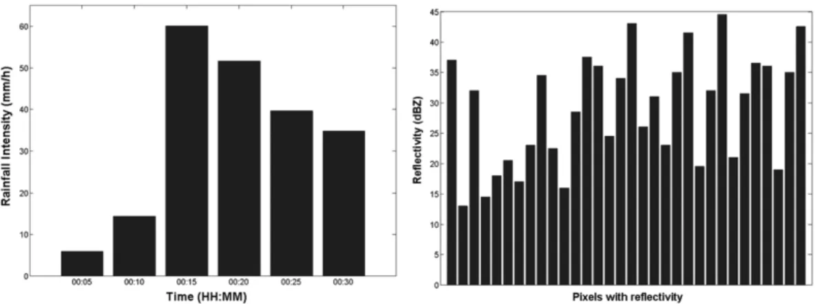
– Firstly, the radar window (3×3 pixels) around the rain gauge is selected (Fig. 3).

– Secondly, each rain gauge’s independent window for every period of 30 min is composed of six 5-minute intensities from SAIH rain gauge (Fig.4a)

10

– Thirdly, each reflectivity’s independent window for every period of 30 min is taken from every pixel (45 in total) coming from five radar windows of each 6-minute radar image (Fig. 4b)

Once the overall dataset of independent windows have been built, the calculation of the Z/R relation could be made from a random sub-sample of that data. To reproduce 15

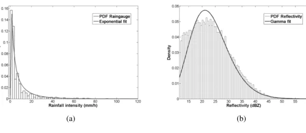
the original method (Rosenfeld et al., 1994) which computed the Z/R relationship by comparing quantiles, a non-parametric technique is used. To avoid problems of tail stability founded in empirical probability distribution function (Kaplan and Meier, 1958), a technique based on a Kernel smoothing density function (Parzen, 1962) is applied. In order to test another smoothed relation, different parametric PDFs were fitted for 20

both rainfall and reflectivity distribution. The ones which maximize the likelihood were exponential function for rain gauge, whereas reflectivity’s PDF is well fitted by Gamma distribution. In Fig. 5, a random sub-sample of 25% of the overall population of win-dows is plotted. Although, the distribution does not fit well for reflectivity values below 19 dBZ, the contribution of this precipitation (less than 0.1 mm/h) can be ignored in 25

(10)

HESSD

7, 7995–8043, 2010

Full Screen / Esc

From both parametric and non-parametric techniques, the derivation of the Z/R rela-tion is very simple and straightforward. This procedure is repeated for various sizes of sub-samples. The minimum population percentage (1%) takes at least 350 values (1% of 36288, which comes from 126 stations∗48 time periods∗6 values). The accuracy of the rainfall intensity that is matched to a specific observed radar reflectivity is evaluated 5

by randomization methods (200 random matches) because every sub-sample gives dif-ferent Z/R relations. This randomization process not only ensures the minimization of spatial and geometrical error, but also provides probabilistic information about the pop-ulation convergence to a final relationship. In this way, Standard Deviation (SD) serves the purpose of assessing the required sample size necessary to obtain a stable Z/R 10

relation (Fig. 6). The SD is also used to evaluate the consistency of the new relation. The bigger the population is, the lower the SD. Due to this trend, the technique of using the mean to get the final relation is absolutely sound.

3.1.2 Stratiform and convective contribution

Adapting the Z/R relationship to different rain types within a given storm or event seems 15

to be a promising way to improve radar QPE (Lee and Zawadzki, 2005). Rosenfeld et al. (1995) improve the accuracy of WPMM estimated rainfall by means of Objective classification criteria based on parameters such as freezing level or bright-band frac-tion. In the present work, the classification criteria is carried out within a 3-D scheme to recognize convective/stratiform areas, developed by Biggerstaffand Listemaa (2000) 20

and based on a previous one (Steiner et al., 1995). These algorithms distinguish be-tween convective and stratiform areas according to reflectivity thresholds and gradients within different CAPPI levels. These thresholds were regionalized to Catalonia by Rigo and Llasat (2004). According to this methodology, in the present paper each different subset of every window is counted in different groups. Therefore, for a same rain gauge 25

intensity window, two radar reflectivity windows are set. This approach to classification criteria results in a non-univocal rain gauge probability distribution function. The fact that a given rainfall intensity could be related to different precipitation types is due to

(11)

HESSD

7, 7995–8043, 2010

Full Screen / Esc

the fact that precipitation type definition is done by vertical velocity scales or genesis (Houze, 1993) and not rainfall intensity. Besides, recorded intensity could not be re-lated to the rain type of the pixel above this rain gauge because of geometrical errors commented previously. Subsequently, non-univocal relation between intensity and rain type should be calculated as two independent univocal datasets. Once all convective 5

and stratiform types have been constructed, the procedure described above is applied to obtain two new Z/R relations for different rain regimes.

3.1.3 Advection correction

The temporal sampling effect of the radar observations can lead to significant errors in the estimated accumulation rainfall as shown in several studies (Liu and Krajewski, 10

1996). To correct this source of error, Anagnostou and Krajewski (1999) proposed an advection correction method based on a cross-correlation technique. This procedure could be applied not only to correct this rainfall estimation, but also for the purpose of increasing the time resolution. For this reason, instead of calculating the cross-correlation coefficient between the two whole images, the first image is divided into 15

a number of template tiles (Fig. 7a). Each template window will be searched for in the second image by using a search window (dashed line in Fig. 7a and 7b), whose size depends on the maximum storm speed that is expected between two sequential images. In the present work this technique was used to obtain the advective displace-ment vector (vector in Fig. 7b), as the vector which maximizes the normalized spatial 20 cross-correlation functionr(p,q). r(p,q)= 1 σ_Aσ_B× X X {[A(x,y)−A(x,y)]· ·[B(x+p,y+q)−B(x+p,y+q)]}= =Cov(p,q) σ_Aσ_B (2)

(12)

HESSD

7, 7995–8043, 2010

Full Screen / Esc

where the pixel values of the template window areA(x,y), and the corresponding pixels in the second window areB(x,y)at no lag andB(x+p,y+q)for a lag(p, q). A(x,y) and B(x+p,y+q) correspond to the mean rainfall values of each window, and σ_A and σ_B are the standard deviations. The displacement(p,q)at the maximum value of the cross correlation determines the advective displacement vector, signifying a storm or cell 5

movement (Dransfeld et al., 2006). This could be described by an advective velocityc [km/h] and displacement angleθ, which are defined by the following equations:

c=[(pmax·∆x) 2₊ (q_max·_∆y)2]12 ∆t (3) θ=arctanqmax·∆y p_max·∆x (4) wherep_maxandq_maxrepresent the spatial displacement in a grid of∆x×∆ypixel size. 10

∆tis the time interval between both images.

Once the advective displacement vector has been obtained by this method, the shape morphology transformation is carried out by means of temporal weights based on a more complex shape transformation (Turk and O’Brien, 2005). Both images, first and second, are extrapolated by means of the computed velocity to the same temporal 15

interval. Then the pixel value is calculated as the temporal-weighted sum of the two images as shown in the next function:

R(x,y,t)= 1 T2· X n (T−t)·Ae(t)+t·Be(t) o (5) where the transformated fieldAeandBeare calculated as a time function by:

e A(t)=A x−t T ·c·cosθ,y− t T ·c·sinθ (6) 20 e B(t)=B x+T−t T ·c·cosθ,y+ T−t T ·c·sinθ (7)

(13)

HESSD

7, 7995–8043, 2010

Full Screen / Esc

whereT [hour] is the original time resolution of radar.

The template size selected is 10×8 pixels whereas the search window for the sec-ond image is 16×14 pixels. This size was calculated taking into account a maximum storm movement lower than 140 km/h following the works of Steinacker et al. (2000) and Rigo (2004). Fig. 8 shows the downscaling from 6 min to 1 min.

5

3.2 Hydrological modeling

3.2.1 Real-Time Interactive Basin Simulator (RIBS)

The Real-time Interactive Basin Simulator (RIBS) is a topography-based, rainfall-runoff model which can be used for real-time flood forecasting in midsize and large basins (Garrote and Bras, 1995). The use of this model is especially attractive in connection 10

with a meteorological radar and distributed rainfall forecasting methods. The RIBS model is largely based on the detailed topographical information provided by digital elevation models (DEM). Basin representation adopts the rectangular grid of the DEM, and other soil properties, input data and state variables are also represented as data layers using the same scheme. The basic objective is to map the topographically driven 15

evolution of saturated areas as the storm progresses. Two modes of runoffgeneration are simulated: infiltration excess runoffand return flow. RIBS applies a kinematic model of infiltration to evaluate local runoffgeneration in grid elements, and also accounts for lateral moisture flow between elements in a simplified manner.

Saturated hydraulic conductivity is assumed to increase with depth, following the 20

relation: K_S

y(y)=K0n·e

−f y ₍₈₎

whereK₀_n [mm h−1] is the saturated hydraulic conductivity at the surface in the direc-tion normal to the surface,y [mm] is depth andf [mm−1] is a parameter that controls the reduction of saturated hydraulic conductivity with depth. There is an anisotropy 25

(14)

HESSD

7, 7995–8043, 2010

Full Screen / Esc

between the hydraulic conductivity in the directions normal and parallel to the soil sur-face, described by the anisotropy ratioα:

α=K0p

K₀_n (9)

whereK₀_p[mm h−1] is the saturated hydraulic conductivity at the surface in the direction parallel to the surface

5

Flow propagation to the basin outlet is computed through distributed convolution, using as instantaneous response function for each element a Dirac delta function, with a delay equal to the time of travel from the location of the element to the basin outlet.

To obtain the travel time to the basin outlet, the speeds for hillslope (v_h) and stream (v_s) must be defined. Stream velocity is assumed to depend on discharge at the basin 10

outlet:

v_s(t)=C_v[Q(t)]r (10)

wherev_s(t) [m/s] is stream velocity at time t,Q(t) is the discharge [m3/s] at the basin outlet and timet, andC_v andr are parameters.

Hillslope velocity is related to stream velocity through the parameterK_v: 15

K_v=vs(t)

v_h(t) (11)

wherev_h(t) [m/s] is hillslope velocity at timetandK_v is a parameter.

The model captures the main features of runoffgeneration processes in watersheds while keeping computational efficiency for real-time use.

3.2.2 Rainfall data into RIBS Hydrological model

20

The RIBS model needs rainfall input data, which are mapped to the rectangular grid of the DEM, or other soil properties. Because of the fact that radar image and DEM res-olutions are different and may correspond to different projections, a preliminary treat-ment of radar images is required. This treattreat-ment is divided into several steps. The first

(15)

HESSD

7, 7995–8043, 2010

Full Screen / Esc

step is coordinate transformation from Mercator to UTM. This is straightforward using general projection transformation formulas (Snyder, 1987).

The second step is an interpolation to downscale the radar resolution grid (2 km×2 km) into DEM resolution (200 m×200 m). The easiest and quickest way is an ordinary linear interpolation, but this methodology does not preserve exactly the 5

total amount of precipitation over the whole domain due to mismatching grids (Fig. 9). In order to avoid it, another procedure has been developed in the present work. As shown in Fig. 9, some DEM grid cells are divided into two different reflectivity parts (grey cell). The main purpose of the new procedure is to preserve the total areal pre-cipitation amount and it is achieved by an area-weighted interpolation. This could be 10

formulated for the example cell as:

R_f=Subareapixel1·Rpixel1+Subareapixel2·Rpixel2

Area DEM grid pixel (12)

or in a general way as: R_f=

P

Subarea_pixel i·Rpixeli

Area DEM grid pixel (13)

Once rain rated for every cell of the whole domain has been calculated by this area-15

weighted interpolation, the Bes `os basin shape is cut out from the high resolution rainfall image.

3.2.3 Probabilistic calibration

The distributed RIBS model was calibrated in the Bes `os basin with the first three ob-served events, and validated with the last obob-served event.

20

Basin shape and location of gauging stations are shown in Fig. 2, and their ba-sic properties are presented in Table 2. The model was calibrated using data from the Gramenet station, very near the basin outlet. The model was validated for the Gramenet station and five other gauge stations which were not used for calibration:

(16)

HESSD

7, 7995–8043, 2010

Full Screen / Esc

Llic¸a station in the Tenas river, Montcada station in the Ripoll river, just upstream its confluence with the Bes `os river, Garriga station in the Congost river, Mogent station in the Mogent river and Mogoda station in the Caldas river.

A probabilistic calibration methodology was applied to obtain the probability density functions of calibration model parameters, which take into account their inherent vari-5

ability. The probabilistic calibration methodology can be summarized as follows: Firstly, a sensitivity analysis was carried out over the calibration parameters of the RIBS model. The observed rainfall data in the first episode in August of 2005 was given as input, and calibration parameter values were randomized. A modification of the GSA methodology proposed by Freer et al. (1996) was applied. This analysis showed 10

that the most influential parameters in the model output are: the rate of variation of the hydraulic conductivity in depth (f), the soil anisotropy coefficient (α), the ratio of hillslope flow velocity to channel flow velocity (K_v) and the coefficient of the law that relates hillslope flow velocity to discharge in the basin outlet (C_v). The antecedent moisture content in the basin is also an influential factor, although it is not a model 15

parameter.

Secondly, the proper calibration was carried out over the first three recorded episodes. A large set of synthetic hydrographs was generated by repetitive simula-tions of the RIBS model for each episode. In this second step, the values of the most influential model parameters were randomized.

20

As the model utilization is the prediction of flash floods, Root Mean Square Error (RMSE), Mean Absolute Error (MAE) and Nash and Sutcliffe Efficiency Coefficient (NSE) were selected (14–16). The NSE coefficient was used to assess the predic-tive power of the simulations (Nash and Sutcliffe, 1970).

RMSE= v u u t 1 T s· T s X t=1 Qt_o−Qt_s2 (14) 25

(17)

HESSD

7, 7995–8043, 2010

Full Screen / Esc

Printer-friendly Version Interactive Discussion Discussion P a per | Dis cussion P a per | Discussion P a per | Discussio n P a per | MAE= T s X t=1 Qt_o−Qt_s (15) NSE=1− PT s t₌1 Qt_o−Qt_s2 PT s t=1 Q_ot−Q_o 2 (16)

whereQt_o is the observed discharge at timet,Q_st is the simulated discharge at timet, Q_ois the mean of observed discharges in the event andT sis the total number of time steps.

5

In a multiobjective calibration no single solution can minimize all the objective func-tions at the same time (Gupta et al., 1998). Therefore, the Pareto solufunc-tions were iden-tified, in order to find the set of non-inferior solutions (Yapo et al., 1998).

Finally, each model parameter was represented by a probability density function (pdf) fitted from the set of Pareto solutions. The distribution functions that best fit the variabil-10

ity of each parameter were identified by means of goodnessof-fit tests, i.e. Chi-Squared test and Kolmogorov-Smirnov test.

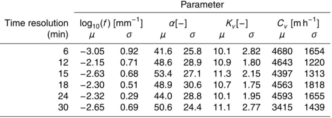
A sensitivity analysis was carried out on the time resolution of precipitation. Spa-tially distributed precipitations were constructed for each event by summing the new advected radar rainfall estimation with a time resolution of one minute. Six time res-15

olutions were selected for the analysis: 30, 24, 18, 15, 12 and 6 min. The calibration methodology was carried out for each rainfall time resolution, in order to take into ac-count that some hydrological parameters may be dependent on time scale. The main statistics of the distribution of parameter values for each time resolution are presented in Table 3.

(18)

HESSD

7, 7995–8043, 2010

Full Screen / Esc

Printer-friendly Version Interactive Discussion Discussion P a per | Dis cussion P a per | Discussion P a per | Discussio n P a per | 3.3 Methods of validation 3.3.1 Radar rainfall

To evaluate the accuracy of radar rainfall estimation three error indexes are calcu-lated. These are BIAS (17), Root Mean Square Error (18) and Mean Error (19). BIAS, which is a relative error, provides information about the total amount of precipitation. 5

Mean error [mm] defines if rainfall is under/over-estimated. RMSE [mm] determines the soundness of estimation gauge by gauge.

BIAS=log· P ·R_i P_· P_i (17) RMSE= s P (R_i−P_i)2 n_i (18) Error= P (R_i−P_i) n_i (19) 10

whereR_i andP_i are the daily rainfall accumulation derived from the radar and registred by XEMA rain-gauges respectively.

3.3.2 Hydrological modelling

Probabilistic calibration leads to a pdf that represents the variability of each parameter. Therefore, the model result is an ensemble distribution of discharges at each time step, 15

which is obtained by generating a large enough number of hydrographs sampling from parameter space. The required number of simulations was defined through a sensitivity analysis. As shown in Fig. 10, a stabilization of results is reached in a range of 150 to 200 simulations. Therefore, 200 model simulations were carried out to validate the model, randomizing each model parameter from the pdf obtained in the calibration. 20

(19)

HESSD

7, 7995–8043, 2010

Full Screen / Esc

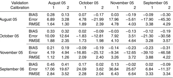
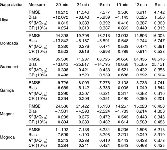
The validation was carried out over the last observed episode. Differences between the validation set and the observed hydrograph were quantified by four measures. Firstly, two of the measures used for calibrating the model were selected, i.e. RMSE and MAE, to measure the accuracy of the simulations. Two other measures were added to improve the validation assessment. Estimation bias was quantified by the 5

Nash-Sutcliffe global efficiency index (R2 (MQ₀_.₅) (Eq. 20), which measures the utility of the median as a forecast (Xiong and O’Connor, 2008). The prediction capability of the calibrated model was quantified by the Containing Ratio (CR) (Eq. 21), which mea-sures the number of observations that are not held between the prediction intervals linked to a given confidence level (Montanari, 2005).

10 R2(MQ₀_.₅)=1.0− T s P t=1 [Qt₀−MQt₀_.₅]2 T s P t=1 [Qt₀−Q₀] (20)

whereT sis the number of time steps, Qt₀ is the observed discharge at time t, MQt₀_.₅ is the median of simulated discharges at timet andQ₀ is the mean of observed dis-charges. CR(α)= P I[Q₀t] T s (21) 15

whereI[Qt₀] is equal to 1 if the observed discharge at timet holds between the confi-dence interval andαis the confidence level, which was set at 10%.

(20)

HESSD

7, 7995–8043, 2010

Full Screen / Esc

Printer-friendly Version Interactive Discussion Discussion P a per | Dis cussion P a per | Discussion P a per | Discussio n P a per | 4 Results 4.1 WPMM methodology

The four selected heavy rainfall events were produced by very different meteorological causes. For this reason the calibration method previously presented is applied for each case, in such a way that eight Z/R relations were obtained due to two fitting methods 5

for the four case studies. In the next table (Table 4) the eight power-law functions are tested for every case.

The results show a major improvement in the three long cases, which are the Octo-ber, November and September cases. The short case (August) shows results of the order of the ones obtained in Atencia et al. (2008), where several Z/R relationships 10

based on the literature were tested. The new relations reduce the BIAS up to 96% and the Root Mean Square Error by 40%. It could be observed that, for the most part, the most suitable data for the calibration is own case data. Nevertheless, the calibra-tion could be carried out by means of other cases that achieve accurate precipitacalibra-tion estimations, as the results prove.

15

4.2 Advection correction

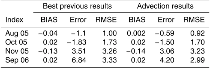
In the next table (Table 5) the results of applying the advection technique to the best rainfall estimation method are shown. For the August case, the best Z-R relation ob-tained in Atencia et al. (2008) was used. In the remaining three cases the matching probabilities method was applied using the gamma function to smooth the probability 20

distribution function. The use of cross-correlation technique to interpolate the rain im-proved the results obtained previously in all the cases for the root mean square error and mean error, but it did not change the total radar rainfall field.

(21)

HESSD

7, 7995–8043, 2010

Full Screen / Esc

4.3 Sensitivity to precipitation time resolution

The model was validated with the last event at six gage stations: Lliça station on the Tenas River, Montcada station on the Ripoll River, just upstream of its confluence with the Bes òs river, Gramenet station on the Bes òs River, very near the basin outlet, Gar-riga station on the Congost River, Mogent station on the Mogent River and Mogoda 5

station on the Caldas River (Fig. 2).

A validation set of 200 simulated hydrographs was generated for each time resolu-tion. These simulated hydrographs were compared with the observed flows for each gauge, obtaining the results presented in Table 6 and Figs. 11 and 12.

The predictive capability for peak discharge is presented in Fig. 11 as a function of 10

rainfall time resolution. Range between confidence limits can be seen as length of the error bars. Most stations show the least variability and the best fit between the median and the observed value for 15 min. In general, the width of the confidence interval and the difference between the median and the observed value increase as rainfall time resolution moves away from 15 min, reaching the maximum in the extreme time 15

resolutions, i.e. 6 and 30 min. 6 and 30 min also show the largest deviations of the median from the observed peak at most stations.

The results obtained for the four validation measures are shown in Fig. 12. To allow for comparison among gauges, RMSE and ME were normalized by observed peak dis-charge. As shown in Fig. 12, minimum RMSE is reached at all stations except Mogoda 20

for 15 min. Model performance is maintained for time resolutions below 12 min, but decreases sharply for time resolutions above 18 min. Minimum absolute value of bias is also for 15 min, but the differences for 12 min are small. Although the figure presents absolute value of bias for the sake of clarity, bias is positive for time resolutions smaller than 15 min and negative for the rest. Gramenet, Montcada and Mogent stations clearly 25

reach the best R2(MQ₀_.₅) for a time resolution of 15 min. Mogoda and Llic¸a stations reach the maximum for 15 min, but there are not great differences with the result for 12 min. Garriga reaches the maximum for 12 min. The behavior of CR shows that most

(22)

HESSD

7, 7995–8043, 2010

Full Screen / Esc

stations reach the maximum for 15 min, except Llic¸a, where the maximum corresponds to 12 min. Maximum ofR2(MQ₀_.₅) and CR is reached in 15 min for most of basins and minimum variability in the peak discharge time step is reached in 15 min for five of six stations.

It seems that the decrease of model performance with increasing time resolution 5

can depend on the maximum time resolution to characterize the rainfall variability in time. This minimum is 15 min, as can be seen in Fig. 12(a–b). The decrease of model performance in validation for time resolutions lower than 15 min can be due to the minimum time resolution required for the hydrological model to characterize the runoff processes. These results lead to 15 min as the best rainfall time resolution for the 10

Bes `os basin, in order to achieve a good representation of rainfall characteristics and a good simulation of hydrological processes.

5 Discussion and conclusions

Distributed hydrological modeling is heavily dependent on spatial distribution of rainfall data. Because of that fact, an effort was made on coupling radar data into a hydrologi-15

cal model in flash-flood cases recorded in Catalonia.

This contribution has been revealed as a good example of the numerous problems that exist in QPE. Firstly, the traditional ZR power-law relationships have not worked well when applied to the selected cases. It is difficult to determine with certainty whether this problem might be associated with poor calibration or maintenance of the 20

radar network or to the attenuation caused by the own heavy precipitation. In order to obtain a suitable QPE, a Window Probability Matching Method (WPMM) and an advection correction have been applied in this work.

Results show that the proposed methodology represents a good improvement of radar rainfall estimation in 75% of the cases. Furthermore, in spite of the dependence 25

of the WPMM on the selected probability distribution fitting function, it has been shown that the rainfall estimation improves with the two tested functions. Accordingly, it is

(23)

HESSD

7, 7995–8043, 2010

Full Screen / Esc

interesting that the minimum root mean square is obtained by fitting parametric func-tions. Initially, the empirical pdf was tested in order to reproduce exactly the original WPMM technique. However, the results not only in the lower tail of the distribution, but also in the higher reflectivity tail show a poor stability over the SD test. For this rea-son, a smooth non-parametric technique (Kernel smooth pdf) was tested. The results 5

improve slightly but the stability is already not high enough. For this reason, several parametric functions have been tested.

The best-fitting parametric functions are the Gamma one for reflectivity and the expo-nential one for rainfall intensity. As is well known, the Gamma function has a potential form multiplied by an exponential function. Because the exponential function does not 10

have the potential factor, the straight relation between rainfall intensity and reflectivity produces a curve of k order in the logarithmic axis. The result of this linear relationship between the two different functions is a non-power-law relation for the transformation of reflectivity in rainfall intensity that increases the quantitative precipitation estimation due to the convex shape of WPMM function in semilog rainfall intensity – reflectivity 15

axis. On the other hand, the smallest bias is usually obtained with non-parametric ker-nel function fitting. In this methodology, both rainfall and reflectivity values are fitted by means of the same function. Moreover, this function is not parametric, but was built by convolution of Gaussian functions. So, the final Z/R shape relation does not have a predefined form due to the linear relation of the function, as happened with parametric 20

functions. The shape obtained by this method is probably the classic power-law rela-tion. Comparing both methodologies, the parametric function provides an increase of lower reflectivity values and a decrease of higher values, whereas the non-parametric methodology produces a similar shape but displaced to the right, which causes a rain-fall intensity increase for all reflectivity values. The second correction made by WPMM 25

non-parametric methodology could be related with a sub-estimation of reflectivity due to the power parameter calibration or own rainfall attenuation.

Taking into account the improvement that involves a convective/stratiform distinction, two Z/R relations are obtained, respectively. This new QPE method gets better results

(24)

HESSD

7, 7995–8043, 2010

Full Screen / Esc

for BIAS index, which means a decrease of the total rainfall field. Furthermore, the new WPMM Z/R relation shape is less convex than the previous one. Accordingly, this approach should be useful for obtaining better QPEs results if a more in-depth rain regime research were carried out.

After that, an advection correction was applied to correct the rainfall amount. It is 5

based on the hypothesis that rainfall intensity is a field in continuous variation. This method is applied in several meteorological services to accumulate the rainfall during an hour. In the present work, this technique was applied to every six radar rainfall fields with two objectives. The first one was to improve the total rainfall estimation; the second was to increase the temporal resolution in order to feed the hydrological model. 10

By applying this method the root mean square error decreased, although bias did not show this behavior. The cause could be the significance of each improvement. The root mean square error is more closely related with the points error, whereas bias is mainly related to the entire rainfall field.

The combined application of both methodologies to correct QPE reduced RMSE by 15

up to 40% and bias between 75% and 95%. These accurate results allow us to couple radar rainfall information across the area-weighted interpolation.

Once a more accurate rainfall field had been obtained for each 6-minute interval, it was entered in the hydrological model. Due to the fact that calibration of distributed hydrological models is strongly dependent on time resolution of rainfall data, the advec-20

tion correction method based on cross-correlation technique was applied to implement a temporal disaggregation in several time resolutions (30, 24, 18, 15, 12, 6 and 2 min). Resolutions lower than 6 min lead to unaffordable computation times for operational hydrological forecasting. Accordingly, only the higher six time resolutions were com-pared. A probabilistic calibration was applied to three case studies in order to obtain 25

the probability density functions that best represent the variability of each model pa-rameter. The calibration was validated with the last episode. This sensitivity analysis of the RIBS model reached the conclusion that a precipitation time resolution of 15 min is recommended for the simulation of the Bes `os catchment. The selected precipitation

(25)

HESSD

7, 7995–8043, 2010

Full Screen / Esc

time resolution compares well with the results presented by (Berne et al., 2004), who studied urban basins up to 100 km2and found a strong relationship between basin size and minimum required rainfall spatial and temporal resolution. They suggested for their upper limit of 100 km2a rainfall minimum temporal resolution of 12 min. The basins an-alyzed in this work range from 100 to 1000 km2and present an optimum time resolution 5

between 12 and 15 min. The results also suggest a lower dependence of rainfall reso-lution from basin size for the range analyzed, which could also be extrapolated to larger basins. Furthermore, the optimum rainfall resolution time could be related with the lag time that would be obtained for a basin with an average slope for the Bes `os Basin and 2 km distance of radar pixel as longitude.

10

This work proved that the highest available rainfall time resolution does not necessar-ily provide the best results in terms of predictive capability of peak flow while the radar system is coupled with a distributed hydrologic model. For the optimum time resolution of 15 min, an RMSE average improvement of 16% was obtained for all sub-basins ana-lyzed when compared to the 6 min time resolution case, with values larger than 10% for 15

all individual basins. Results for other basins could vary across the Mediterranean, due to the influence on basin response of other characteristics not analyzed in this work, such as geomorphology, geology, vegetation, etc. Therefore, a previous analysis of the optimum rainfall time resolution is recommended in order to improve performance of real-time flash flood forecasting schemes.

20

Acknowledgements. This research is supported by the Sixth Framework Programme European

Commission FLASH project (n.036852). It is also included in the framework of the Spanish Severus project (CGL2006-13372-CO2-02). The authors thank Meteocat (Catalan Meteoro-logical Service) for its rainfall data from the XAC and XMET networks and radar data from the XRAD network. Thanks to ACA (Catalan Water Agency) for the rainfall and stream flow

25

data from the SAIH network. The authors also wish to thank CLABSA for the Bes `os basin information.

(26)

HESSD

7, 7995–8043, 2010

Full Screen / Esc

Printer-friendly Version Interactive Discussion Discussion P a per | Dis cussion P a per | Discussion P a per | Discussio n P a per | References

Anagnostou, E. and Krajewski, W.: Real-time radar rainfall estimation. Part I: Algorithm for-mulation, J. Atmos. Ocean. Tech., 16, 189–197, doi:10.1175/1520-0426(1999)016h0189: RTRREPi2.0.CO;2, 1999. 7998, 8005

Arnaud, P., Bouvier, C., Cisneros, L., and Dominguez, R.: Influence of rainfall spatial variability

5

on flood prediction, J. Hydrol., 260, 216–230, doi:10.1016/S0022-1694(01)00611-4, 2002. 7997

Atencia, A., Ceperuelo, M., Llasat, M., and Vilaclara, E.: A new non power-law Z/R relation in western Mediterranean area for flash-flood events, in: Proceedings of Fifth European Conference on Radar in Meteorology and Hidrology (ERAD)., Helsinki, Finland, 7, p. 14,

10

2008. 8002, 8014

Atlas, D., Rosenfeld, D., Wolff, D., Aeronautics, N., and Space Administration. Goddard Space Flight Center, Greenbelt, M.: Climatologically tuned reflectivity-rain rate relations and links to area-time integrals, J. Appl. Meteorol., 29, 1120–1135, 1990. 8002

Barnolas, M. and Llasat, M. C.: A flood geodatabase and its climatological applications:

15

the case of Catalonia for the last century, Nat. Hazards Earth Syst. Sci., 7, 271–281, doi:10.5194/nhess-7-271-2007, 2007. 7999

Bech, J., Codina, B., Lorente, J., and Bebbington, D.: The sensitivity of single polarization weather radar beam blockage correction to variability in the vertical refractivity gradient, J. Atmos. Ocean. Tech., 20, 845–855, doi:10.1175/1520-0426(2003)020h0845:TSOSPWi2.0.

20

CO;2, 2003. 8001

Bell, V. A. and Moore, R. J.: Short period forecasting of catchment-scale precipitation. Part II: a water-balance storm model for short-term rainfall and flood forecasting, Hydrol. Earth Syst. Sci., 4, 635–651, doi:10.5194/hess-4-635-2000, 2000. 7996

Berne, A., Delrieu, G., Creutin, J., and Obled, C.: Temporal and spatial resolution of rainfall

25

measurements required for urban hydrology, J. Hydrol., 299, 166–179, 2004. 8019

Biggerstaff, M. and Listemaa, S.: An improved scheme for convective/stratiform echo classifica-tion using radar reflectivity, J. Appl. Meteorol., 39, 2129–2150, doi:10.1175/1520-0450(2001) 040h2129:AISFCSi2.0.CO;2, 2000. 8004

Carpenter, T. and Georgakakos, K.: Intercomparison of lumped versus distributed hydrologic

30

model ensemble simulations on operational forecast scales, J. Hydrol., 329, 174–185, doi: 10.1016/j.jhydrol.2006.02.013, 2006. 7997

(27)

HESSD

7, 7995–8043, 2010

Full Screen / Esc

Ceperuelo, M. and Llasat, M.: La Precipitacion Convectiva en las Cuencas Internas de Catalunya, Revista del Aficionado a la Meteorologıa, 23, 2004. 8000

Chapon, B., Delrieu, G., Gosset, M., and Boudevillain, B.: Variability of rain drop size distribu-tion and its effect on the Z–R relationship: A case study for intense Mediterranean rainfall, Atmos. Res., 87, 52–65, doi:10.1016/j.atmosres.2007.07.003, 2008. 8002

5

Delrieu, G., Andrieu, H., and Creutin, J.: Quantification of path-integrated attenuation for X-and C-band weather radar systems operating in Mediterranean heavy rainfall, J. Appl. Meteorol., 39, 840–850, doi:10.1175/1520-0450(2000)039h0840:QOPIAFi2.0.CO;2, 2000. 7997 Dransfeld, S., Larnicol, G., and Le Traon, P.: The Potential of the Maximum Cross-Correlation

Technique to Estimate Surface Currents From Thermal AVHRR Global Area Coverage Data,

10

IEEE Geosci. Rmote. S., 3, 508–511, doi:10.1109/LGRS.2006.878439, 2006. 8006, 8038 Franco, M., S ´anchez-Diezma, R., and Sempere-Torres, D.: Improving radar precipitation

es-timates by applying a VPR correction method based on separating precipitation types, in: Proceedings of Fifth European Conference on Radar in Meteorology and Hidrology (ERAD)., Helsinki, Finland, 14, p. 14, 2008. 7998

15

Freer, J., Beven, K., and Ambroise, B.: Bayesian estimation of uncertainty in runoffprediction and the value of data: An application of the GLUE approach, Water Resour. Res., 32, 2161– 2173, 1996. 8010

Garrote, L. and Bras, R.: A distributed model for real-time flood forecasting using digital ele-vation models, J. Hydrol., 167, 279–306, doi:10.1016/0022-1694(94)02592-Y, 1995. 7998,

20

7999, 8007

Garrote, L., Molina, M., and Mediero, L.: Hydroinformatics in Practice: Computational Intel-ligence and Technological Developments in Water Applications, chap. Learning Bayesian networks from deterministic rainfall–runoff models and Monte-Carlo simulation, 375–388, Springer, doi:10.1007/978-3-540-79881-1 27, 2007. 7998

25

Gupta, H., Sorooshian, S., Yapo, P., et al.: Toward improved calibration of hydrologic models: Multiple and noncommensurable measures of information, Water Resour. Res., 34, 751–763, 1998. 8011

Haddad, Z., Short, D., Durden, S., Im, E., Hensley, S., Grable, M., and Black, R.: A new parametrization of the rain drop size distribution, IEEE Geosci. Rmote. S., 35, 532–539,

30

doi:10.1109/36.581961, 1997. 7997

Houze, R.: Cloud dynamics, 53, San Diego: Academic Press, 1993. 8005

(28)

HESSD

7, 7995–8043, 2010

Full Screen / Esc

the American statistical association, 53, 457–481, doi:10.2307/2281868, 1958. 8003 Krajewski, W., Lakshmi, V., Georgakakos, K., and Jain, S.: A Monte Carlo study of rainfall

sampling effect on a distributed catchment model, Water Resour. Res., 27, 119–128, doi: 10.1029/90WR01977, 1991. 7997

Lee, G. and Zawadzki, I.: Variability of drop size distributions: Time-scale dependence of the

5

variability and its effects on rain estimation, J. Appl. Meteorol., 44, 241–255, doi:10.1175/ JAM2183.1, 2005. 7997, 8004

Liu, C. and Krajewski, W.: A comparison of methods for calculation of radar-rainfall hourly accu-mulations, J. Am. Water Resour. As., 32, 305–315, doi:10.1111/j.1752-1688.1996.tb03453. x, 1996. 8005

10

Llasat, M., Rigo, T., and Barriendos, M.: The Montserrat-2000 flash-flood event: a compari-son with the floods that have occurred in the northeastern Iberian Peninsula since the 14th century, Icon-Int. J. Const. Law., 23, 453–469, doi:10.1002/joc.888, 2003. 7999

Llasat, M. C., L ´opez, L., Barnolas, M., and Llasat-Botija, M.: Flash-floods in Catalonia: the social perception in a context of changing vulnerability, Advances in Geosciences, 17, 63–

15

70, 2008. 8000

Madsen, H.: Parameter estimation in distributed hydrological catchment modelling using au-tomatic calibration with multiple objectives, Adv. Water Resour., 26, 205–216, doi:10.1016/ S0309-1708(02)00092-1, 2003. 7998

Marshall, J. and Palmer, W.: The distribution of raindrops with size, J. Atmos. Sci., 5, 165–166,

20

doi:10.1175/1520-0469(1948)005h0165:TDORWSi2.0.CO;2, 1948. 7997

Mediero, L., Garrote, L., and Martin-Carrasco, F.: A probabilistic model to support reservoir operation decisions during flash floods/Un modele probabiliste d’aide a la decision pour la gestion d’un reservoir lors de crues eclairs, Hydrolog. Sci. J., 52, 523–537, doi:10.1623/hysj. 52.3.523, 2007. 7998

25

Montanari, A.: Large sample behaviors of the generalized likelihood uncertainty estimation (GLUE) in assessing the uncertainty of rainfall-runoffsimulations, Water Resour. Res., 41, W08406, doi:10.1029/2004WR003826, 2005. 8013

Morin, E. and Gabella, M.: Radar-based quantitative precipitation estimation over Mediter-ranean and dry climate regimes, J. Geophys. Res-Atmos., 112, D20 108, doi:10.1029/

30

2006JD008206, 2007. 7998

Morin, E., Enzel, Y., Shamir, U., and Garti, R.: The characteristic time scale for basin hydrologi-cal response using radar data, J. Hydrol., 252, 85–99, doi:10.1016/S0022-1694(01)00451-6,

(29)

HESSD

7, 7995–8043, 2010

Full Screen / Esc

Printer-friendly Version Interactive Discussion Discussion P a per | Dis cussion P a per | Discussion P a per | Discussio n P a per | 2001. 7999

Nash, J. and Sutcliffe, J.: River flow forecasting through conceptual models. part I-A discussion of principles, J. Hydrol., 10, 282–290, doi:10.1016/0022-1694(70)90255-6, 1970. 8010 Parzen, E.: On estimation of a probability density function and mode, The Annals of

Mathemat-ical Statistics, 33, 1065–1076, doi:10.1214/aoms/1177704472, 1962. 8003

5

Refsgaard, J.: Parameterisation, calibration and validation of distributed hydrological models, J. Hydrol., 198, 69–97, doi:10.1016/S0022-1694(96)03329-X, 1997. 7998

Rigo, T.: Estudio de sistemas convectivos mesoescalares en la zona mediterr ´anea occidental mediante el uso del radar meteorol ´ogico, Ph.D. thesis, PhD thesis, University of Barcelona, Internal publication, 2004. 8002, 8007

10

Rigo, T. and Llasat, M. C.: A methodology for the classification of convective structures using meteorological radar: Application to heavy rainfall events on the Mediterranean coast of the Iberian Peninsula, Nat. Hazards Earth Syst. Sci., 4, 59–68, doi:10.5194/nhess-4-59-2004, 2004. 8004

Robinson, J., Sivapalan, M., and Snell, J.: On the relative roles of hillslope processes,

chan-15

nel routing, and network geomorphology in the hydrologic response of natural catchments, Water Resour. Res., 31, 3089–3101, doi:10.1029/95WR01948, 1996. 7999

Rosenfeld, D., Wolff, D., and Atlas, D.: General probability-matched relations between radar reflectivity and rain rate, J. Appl. Meteorol., 32, 50–72, doi:10.1175/1520-0450(1993) 032h0050:GPMRBRi2.0.CO;2, 1993. 8002

20

Rosenfeld, D., Wolff, D., and Amitai, E.: The window probability matching method for rainfall measurements with radar, J. Appl. Meteorol., 33, 682–693, doi:10.1175/1520-0450(1994) 033h0682:TWPMMFi2.0.CO;2, 1994. 7998, 8002, 8003

Rosenfeld, D., Amitai, E., and Wolff, D.: Improved accuracy of radar WPMM estimated rainfall upon application of objective classification criteria, J. Appl. Meteorol., 34, 212–223, doi:

25

10.1175/1520-0450(1995)034h0212:IAORWEi2.0.CO;2, 1995. 8004

S ´anchez-Diezma, R., Zawadzki, I., and Sempere-Torres, D.: Identification of the bright band through the analysis of volumetric radar data, J. Geophys. Res.-Atmos., 105, 2225–2236, doi:10.1029/1999JD900310, 2000. 7997

S ´anchez-Diezma, R., Sempere-Torres, D., Delrieu, G., and Zawadzki, I.: An improved

method-30

ology for ground clutter substitution based on a pre-classification of precipitation types, in: 30 th Internat. Conf. on Radar Meteor, 271–273, Munich, Germany, 2001. 7997