http://dx.doi.org/10.4236/msce.2016.43001
How to cite this paper: Hammi, H., El Ouafi, A. and Barka, N. (2016) Study of Frequency Effects on Hardness Profile of Spline Shaft Heat-Treated by Induction. Journal of Materials Science and Chemical Engineering, 4, 1-9.
http://dx.doi.org/10.4236/msce.2016.43001
Study of Frequency Effects on Hardness
Profile of Spline Shaft Heat-Treated
by Induction
Habib Hammi, Abderazzak El Ouafi
*, Noureddine Barka
Mathematics, Computer Science and Engineering Department, University of Quebec at Rimouski, Rimouski, Canada
Received 30 January 2016; accepted 6 March 2016; published 9 March 2016
Copyright © 2016 by authors and Scientific Research Publishing Inc.
This work is licensed under the Creative Commons Attribution International License (CC BY). http://creativecommons.org/licenses/by/4.0/
Abstract
This paper is devoted to the study of frequency effects on hardness profile of AISI 4340 spline shaft heat-treated by induction through an extensive 3D finite element method simulation and structured experimental investigation. Based on coupled electromagnetic and thermal fields analysis, the 3D model is used to estimate the temperature distribution and the hardness profile. The proposed study examines the hardening process parameters, such as frequency, induced cur-rent density and heating time, known to have an influence on hardened surface and builds the si-mulation model step by step. The established model can provide not only an accurate prediction of temperature distribution and hardness profile but also a comprehensive analysis of machine pa-rameters effects, especially the frequency. The numerical results achieved by this model are good and present a great agreement to the experimental data.
Keywords
Induction Heating, Splines Shaft, Hardness Profile, Current Density, Heating Time, Frequency
1. Introduction
Surface transformation hardening processes are designed to improve wear and fatigue resistance by hardening the superficial critical areas using brief and localized heat gains. Among these processes, induction heating process is well-known by its capacity in terms of high power density which allows short interaction times to reach the required temperature, while limiting the risks of undesirable distortion and deformation effects [1] [2].
Induction heating consists of heating an electrically conducting part by applying an alternative current at a spe-cific frequency into a copper coil to produce a variable electromagnetic field, which generates induced eddy currents in the region, close to the coil. The eddy currents flowing through the resistance of the part, placed within the coil, heat it by Joule effect. The induction heating process exhibits several industrial advantages: i) requires low energy levels; ii) minimizes distortion and deformation of the heated parts; iii) easily to integrate in automated production lines and iv) considered as a sustainable manufacturing process [1] [2]. The mechanical characteristics of the hardened surface obtained by this process depend on the physicochemical properties of the treated material and several induction heating parameters and conditions. To be able to appropriately use the re-sources offered by an induction heating system, it is necessary to develop a comprehensive strategies to control the heating process parameters in order to produce desired hardened surface characteristics for a specific appli-cation. Despite some attempts to develop models and approaches to study typical aspects of the induction heat-ing, the developed simulation tools and strategies are not flexible enough to be applied to various materials and geometries [3]-[5]. Current practices in the industry are based on the control the induction heating process using handbook data and the traditional and fastidious trial and error procedures for every single specific mechanical component. There are no general studies that document and predict the performance of the process as function of heating system parameters.
The efficiency of an induction heating system for typical application depends on several factors such as char-acteristics of the mechanical part itself (material and geometry), inductor design and heating system parameters (power supply capacity, frequency, induced current density, heating time, etc.) [2]-[6]. It is very well known that the penetration depth is proportional to the inverse of the frequency, leading to a comprehensive study of the difference between using a high frequency (HF) and medium frequency (MF) current in the heating process. Furthermore, to obtain an adequate temperature distribution and uniform hardness profile, in the case of the spline shaft treatment, a specific frequency is required to qualify the induced current to reach the tooth and the root zones. Relationship between the resulting temperature and the frequency used has to be established.
In this work, a coupled electromagnetic fields and thermal analysis 3D numerical model for AISI 4340 steel spline shaft is designed using COMSOL multi-physics software. Various induction heating parameters such as frequency, induced current density and heating time are tested and their effects on temperature distribution and hardness profile are evaluated. The 3D model subsequently used specifically to establish and evaluate the con-tribution of the frequency variation on the heating process performance. The numerical results achieved by the 3D model are validated using relevant experimental data.
2. Problem Formulation and Simulation
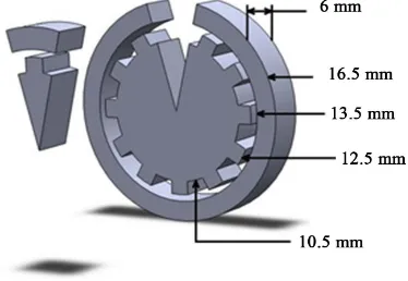
[image:2.595.219.406.574.703.2]The proposed simulation 3D model uses a 25 mm external diameter AISI 4340 steel spline with 21 mm internal diameter. The spline is wound with a 27 mm copper based coil (Figure 1). Because of the circular symmetry of the shaft, only one twelfth of the spline and the coil are considered in the simulation model (the spline is com- posed of twelve teeth). These parameters are chosen taking into account the constraints imposed by the experi-mental setup and conditions (heating system and geometry of the available mechanical parts). The AISI 4340 alloy steel used is a low alloy steel that contains iron (95.195% - 96.33%), nickel (1.65% - 2%), chromium (0.7% - 0.9%), manganese (0.6% - 0.8%), carbon (0.37% - 0.43%), molybdenum (0.2% - 0.3%), silicon (0.15% - 0.3%), sulfur (0.04%) and phosphorous (0.035%). This steel is heat treated at 830˚C followed by quenching in
oil. The analysis assumes that the ambient temperature is set to 293 K and that the spline and the coil are sur-rounded by a local dielectric environment that is magnetically isolated with vacuum permittivity and permeabil-ity.
2.1. Problem Formulation
To calculate the electromagnetic field, it is imperative to solve Maxwell’s equations, for generally varying elec-tromagnetic fields. Maxwell’s equations can be written as:
D
H J
t
∂ ∇ × = +
∂ (1)
B E
t
∂ ∇ × = −
∂ (2)
0
B
∇ ⋅ = (3)
charge
D ρ
∇ ⋅ = (4)
Here E is electric field intensity, D is electric flux density, H is magnetic field intensity, B is magnetic flux density, J is conduction current density, and ρcharge is electric charge density. Special symbols like ∇ ⋅ and
∇ × are popular in vector algebra and are useful to shorten an expression of particular differential operations without having to carry out the details. ∇ =U gradU,∇ ⋅ =U divU and ∇ × =U curlU . In this part, we used the Fourier equation as it is written in the following form.
(
)
T
c k T Q
t
γ ∂ + ∇ ⋅ − ∇ =
∂ (5)
T is temperature, γ is the density of the metal, c is the specific heat, k is the thermal conductivity of the met-al and Q is the heat source density induced by eddy currents per unit time in a unit volume. So the system to be solved is given by:
( )
(
1)
0
jωσ T A+ ∇ × µ−∇ ×A = (6)
(
,)
p
T
C k T Q T A
t
ρ ∂ − ∇ ⋅ ∇ =
∂ (7)
where
ρ
is the density, Cp is the specific heat capacity.Induction heating is a non-contact heating process. It uses high frequency electricity to heat materials that are electrically conductive [6]. Since it is non-contact, the heating process does not contaminate the material being heated. It is also very efficient since the heat is actually generated inside the work piece. This can be contrasted with other heating methods where heat is generated in a flame or heating element, which is then applied to the work piece.
A source of high frequency electricity is used to drive a large alternating current through a coil [7]. This coil is known as the work coil. The passage of current through this coil generates a very intense and rapidly changing magnetic field in the space within the work coil. The work piece to be heated is placed within this intense alter-nating magnetic field [6], [8]. The alternating magnetic field induces a current in the conductive work piece. The arrangement of the work coil and the work piece can be thought of as an electrical transformer. The work coil is like the primary where electrical energy is fed in, and the work piece is like a single turn secondary that is short-circuited. This causes tremendous currents to flow through the work piece, known as eddy currents.
In addition to this, the high frequency used in induction heating applications gives rise to a phenomenon called skin effect [6] and [9]. This skin effect forces the alternating current to flow in a thin layer towards the surface of the work piece. The skin effect increases the effective resistance of the metal to the passage of the large current. Therefore it greatly increases the heating caused by the current induced in the work piece. The principle of induction heating is mainly based on two well-known physical phenomena.
E dt
∂∅
= (8)
When the loop is short-circuited, the induced voltage (E) will cause a current to flow that opposes its cause, the alternating magnetic field. This is Faraday-Lenz’s law.
If a “massive” conductor (e.g. a cylinder) is placed in the alternating magnetic field instead of the short cir-cuited loop, eddy currents (Foucault currents) will be induced within it. The eddy currents heat up the conductor according to the Joule effect.
The second phenomena is the Joule effect, wherein a current, I(A) flows through a conductor with a resistance,
( )
R Ω , and the power P W
( )
is dissipated in the conductor according to:2
P=RI (9) A general characteristic of alternating currents is that they are concentrated on the outside of a conductor. This is called the skin effect. Eddy currents induced in the material are also the biggest on the outside and dimi-nish towards the center [10]. Therefore most of the heat is generated on the outside. The skin effect is characte-rized by its so-called penetration depth (
δ
), defined as the thickness of the layer, measured from the outside, in which 87% of the power is developed. The penetration depth can be deduced from Maxwell’s equations. For a cylindrical load with a diameter that is much bigger thanδ
, the formula is as follows:f
ρ δ
π µ
=
⋅ ⋅ (10)
The penetration depth depends on the characteristics of the material to be heated (
µ ρ
, ), and is also influ-enced by the frequency. The frequency dependence offers a possibility to control the penetration depth. As can be derived from the formula above, the penetration depth is inversely proportional to the square root of µr. For nonmagnetic materials like copper or aluminum the relative magnetic permeability is equal to 1.On the contrary, ferromagnetic materials (iron, many types of steel) have a relative magnetic permeability that is much higher. Therefore, these materials generally show a more explicit skin effect (smaller
δ
). The magnetic permeability of ferromagnetic materials strongly depends on the composition of the materials and on the cir-cumstances (temperature, magnetic field intensity, saturation).Above the Curie temperature, µr suddenly drops again to 1, which implies a rapid increase of the penetration depth. The current flow in skin effect can be calculated using equation:0e
x x
i =i − δ (11) where, ix is the current density at x distance from the surface and i0 refers to current density at the skin depth.
2.2. Simulation
Simulations were conducted after establishing the most suitable mesh size to be used. The imposed current den-sity (J0) is adjusted so that T reaches a specific temperature of 1000˚C after 1 s of heating. When the tempera-ture reaches 1000˚C, it is certain that the steel has been transformed to a martensitic form. A primary compari-son is presented in Figure 2 showing the difference between temperature distributions when the frequency in-creases from 50 kHz to 500 kHz. For the following study, Ttip and Troot are measured in the tip and the root of the tooth of the spline, as shown in Figure 2(c). In those two regions, the spline is in contact with other me-chanical components and friction is elevated.
3. Effect of Frequency and Heating Time on Temperature Distribution
Figure 2. Temperature distributions (˚C) for different frequency. (a) 50 kHz; (b) 100 kHz; (c) 150 kHz; (d) 200 kHz; and (e) 500 kHz.
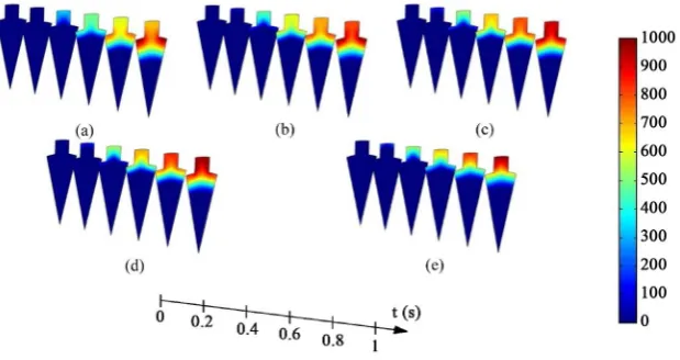
Figure 3. Evolution of temperature distribution (˚C) versus heating time for different frequency. (a) 50 kHz; (b) 100 kHz; (c) 150 kHz; (d) 200 kHz; and (e) 500 kHz.
of the spline. See Figure 3(c). For a frequency of 200 kHz, the induced currents are concentrated at the tooth tip and flank with some heat generated at the root. The skin depth is less than when MF is used. See Figure 3(d). When the frequency increases to 500 kHz (VHF), as shown inFigure 3(e), the skin depth becomes very small compared to that seen with HF and MF. The induced currents do not sufficiently penetrate the spline. The only region where the temperature reaches 1000˚C is the upper tip of the teeth. In conclusion, the frequency affects the temperature profile by changing the skin depth. When the frequency increases, the skin depth decreases. When the skin depth decreases, the temperature profile becomes narrower and is more restricted to the tooth tip.
High frequency induction heating has a shallow skin effect, which is more efficient for small parts, and low frequency induction heating has a deeper skin effect, which is more efficient for larger parts. As a rule, heating smaller parts requires higher operating frequencies (often greater than 50 kHz), and larger parts are more effi-ciently heated with lower operating frequencies. Temperatures at the tip and at the root are calculated for all frequencies and are shown in Table 1.
The effect of heating time over temperature distribution is the same at all five frequencies. The temperature increases when the heating time increases. At the beginning of the process, the heat is concentrated in a minor region and starts to spread as the time increases. In the case of MF, the heat started to spread outward from the root without touching the tip. In the case of HF, it started in the flank and spread without touching the root. Fi-nally, in the case of VHF, it started from the tip and spread just through the tip of the tooth.
[image:5.595.159.469.276.440.2]strated in Figure 4(a). As the frequency increases, the hardened region migrates from the root toward the ex-treme tip of the spline tooth as demonstrated in Figures 4(b)-(e). This is due to the skin effect and equation 10.
It is important to analyze the effect of frequency on temperature at the end of the heating period (t = 1 s). Af-ter measuring the temperature at the tip and root for all frequencies (Table 1), it is seen that these two tempera-tures intersect at a frequency of 180 kHz as illustrated in Figure 5. This means that for a frequency of 180 kHz and for a specific J0, the temperature at the tip and at the root must be equal, which means that the temperature profile should be uniform. It is also observed that the imposed current density (J0) increases when the frequen-cy increases. The values of J0 for 50 kHz, 100 kHz, 150 kHz, 200 kHz, and 500 kHz are respectively equal to
10 2 10
1.99× A m , 10 2
10
2.70× A m , 10 2
10
3.21× A m , 10 2
10
3.57× A m , and 10 2 10
5.11× A m .
4. Prediction of the Hardened Profile and Validation
As seen in the previously, the frequency that gives the uniform temperature distribution is equal to 180 kHz. This frequency value is used to find the correct induced current density that meets the criteria leading to uniform temperature distribution. As illustrated clearly inFigure 6, when frequency is equal to 180 kHz, J0 should be equal to 3.4275×10¹⁰A m2. Those two parameters are used to build the simulation that should yield a uniform temperature distribution, and will be compared to the experimental results.
4.1. Prediction of the Hardened Profile
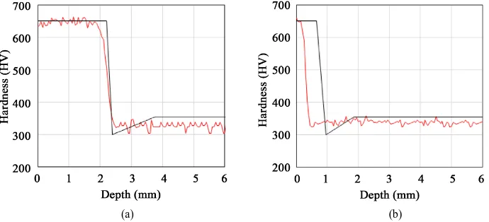
The AISI 4340 spline has a high core hardness, HC, which means that the microstructure is in an unstable martensitic state. From the surface to dS, the region is transformed to an austenitic phase because the tempera-ture T is greater than Ac3. This region is transformed to a martensitic structure and is characterized by a maxi-mum hardness called HS. The second region represents a loss in hardness and is characterized by a minimum hardness value called HL. The third region is heated but not transformed because the temperature is less than
1
Ac . Finally the fourth region corresponds to the zone that is not affected by the transformations. The case depth is characterized by the first zone called hard zone. In fact, a case depth being at full hardness is interesting to consider as a specification since there would be a homogeneous microstructure, nearly uniform hardness, and compressive residual stresses levels [11].
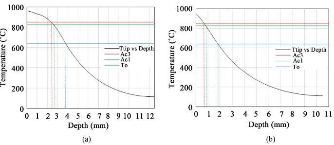
The four region limits are calculated inFigure 7(a) for the tip andFigure 7(b) for the root. In fact, it is suffi-cient to calculate the x-axis coordinates of the points at the intersections of the temperature versus depth curve and Ac3, Ac1 and T0. Ac3 is the temperature above which the material is transformed to a martensitic form,
1
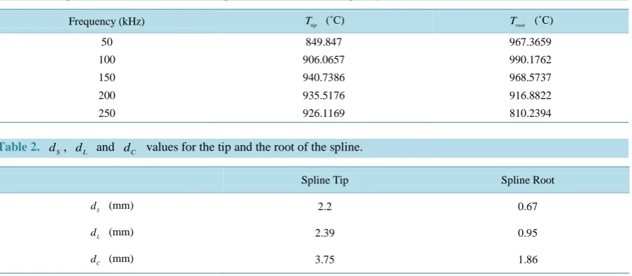
Ac is the temperature at which the transformation starts, and T0 is the maximum value of the temperature at which the AISI 4340 does not undergo any change in its micro-structure.Table 2 shows the measured values of,
S
[image:6.595.89.541.525.722.2]d , dL and dC for the tip and the root of the spline.
Table 1. Temperature measurements in the tip and the root versus frequency.
Frequency (kHz) Ttip (˚C) Troot (˚C)
50 849.847 967.3659
100 906.0657 990.1762
150 940.7386 968.5737
200 935.5176 916.8822
250 926.1169 810.2394
Table 2. dS, dL and dC values for the tip and the root of the spline.
Spline Tip Spline Root
S
d (mm) 2.2 0.67
L
d (mm) 2.39 0.95
C
Figure 4. Predicted hardened profile for different frequency. (a) 50 kHz; (b) 100 kHz; (c) 150 kHz; (d) 200 kHz; (e) 500 kHz.
Figure 5. Temperature versus frequency for the tip (blue) and the root (red).
Figure 6. Induced current density versus frequencies.
(a) (b)
[image:7.595.210.432.379.527.2] [image:7.595.144.487.554.703.2]The horizontal hardness value of the first region demonstrates that it was transformed to a martensitic struc-ture. The hardness drops dramatically in the second region. In this region, the material tries to affect a reaction opposing the action of heating, and the hardness reaches a minimal value. In the third region, the hardness value increases again to its initial value. This is normal, as it is closer to the core. The last region represents the ma-terial with unaffected microstructure. Both the tip and the root surfaces are hardened using a single frequency current. The spline is hardened in the surface and not in the core. The core hardness does not change. This is normal for surface treatment, which is meant to be the most concentrated on the surface as it is the region that is always in contact with other components. Since this is the region that will deteriorate the most quickly, hardness must be maximal on the surface and in the skin depth.
Data in Table 2is used to representthe hardnessversus depth curve from the surface to the core. These curves are compared to the ones resulting from the micro measurements of the heated specimen. Graphs in Figure 8
show that the hardness is predicted with an excellent accuracy between d = 0 mm to d = ds. The measured
hard-ness present uniform profiles along the maximum hardened region.
From dL to dC, the hardness drops dramatically to its minimum value. This region constitutes the boun-dary between the hardened and the non-hardened regions. Outside of it, the material is transformed, rigid and hardened so that it is able to withstand continual contact with other components and failure. On the contrary, the inside of the spline (closer to the core) is non-hardened and maintains its original hardness, giving some degree of flexibility to the mechanical component that helps to prevent cracks from forming. In the final zone, the ma-terialdoes not undergo any transformation, and carbon does not change the original AISI 4340 microstructure.
The predicted model is very accurate in the tip of the spline tooth, as opposed to in the root where results are not very similar. In fact, the predicted hardness in the root is slightly delayed, in terms of depth, from the meas-ured hardness. This is due to edge effects and experimental errors. In the simulation only one twelfth is studied due to symmetrical aspect of the model, but when the real spline was treated there were no edges because the spline was not divided.
4.2. Validation
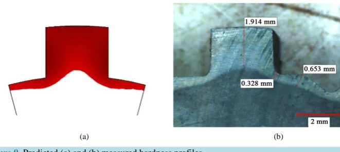
Even with the small error in the root simulation due to edge effects, it is seen that the predicted and the meas-ured hardened regions are quite similar. The machine parameters used in the simulation produced a good har-dened pattern as compared to the real pattern achieved using the induction machine. The results obtained dem-onstrated that the hardened region depends directly on machine parameters. This region can be reduced by using high frequencies and decreasing heating time as depicted inFigure 9.
5. Conclusion
In this work, induction heating process is applied to a spline shaft in order to understand the effect of frequency and heating time on the final temperature distributions and hardness profile. The model used to evaluate the sur- face hardening attributes is based on coupled electromagnetic and thermal fields analysis. The achieved results
[image:8.595.143.488.548.705.2](a) (b)
(a) (b)
Figure 9. Predicted (a) and (b) measured hardness profiles.
establish that the proposed model can provide an accurate prediction of temperature distribution and precise approximation of the hardness profile beside a comprehensive analysis of induction heating parameters effects, especially medium, high and very high frequency currents. The simulation results are validated by data from numerous and structured experiments. The results present a good agreement between simulation and experi-mental data. This work opens an interesting perspective to investigate the use of multi-frequency currents and various design involving multiple coils and scanning processes.
References
[1] Semiatin, S.L. and Stutz, D.E. (1987) Induction Heat Treatment for Steel. 2nd Edition, American Society for Metal, Metals Park, Ohio.
[2] Rudnev, V., Loveless, D., Cook, R. and Black, M. (2003) Handbook of Induction Heating. Marcell Dekker Inc., New York.
[3] Hammi, H., Barka, N. and El Ouafi, A. (2015) Effects of Induction Heating Process Parameters on Hardness Profile of 4340 Steel Bearing Shoulder Using 2D Axisymmetric Model. International Journal of Engineering and Innovative
Technology, 4, 41-48.
[4] Barka, N., El Ouafi, A., Chebak, A., Bocher, P. and Brousseau, J. (2012) Sensitivity Study of Temperature Profile of 4340 Spur Gear Heated by Induction Process Using 3-D Simulation. Journal of Applied Mechanics and Materials, 232, 736-741. http://dx.doi.org/10.4028/www.scientific.net/AMM.232.736
[5] Chebak, A., Barka, N., Menou, A., Brousseau, J. and Ramdenee, D.S. (2011) Simulation and Validation of Spur Gear Heated by Induction Using 3D Multi-Physics Model. World Academy of Science, Engineering and Technology, 59, 893-897.
[6] Zinn, S. and Semiatin, S.L. (1988) Elements of Induction Heating: Design, Control, and Applications. ASM Interna-tional, Metals Park, Ohio.
[7] Lin, C.Y., Wu, M., Bloom, J.A., Cox, I.J. and Miller, M. (2001) Rotation, Scale, and Translation Resilient Public Wa-termarking for Images. IEEE Transactions on Image Process, 10, 767-782. http://dx.doi.org/10.1109/83.918569
[8] Lienhard IV, J.H. and Lienhard V, J.H. (2008) A Heat Transfer Textbook. Phlogiston Press, Cambridge, Massachu-setts.
[9] Jungwirth, M. and Hofinger, D. (2007) Multiphysics Modelling of High-Frequency Inductive Device. The Proceeding
of the COMSOL Users Conference, Grenoble, 2007.
[10] Li, M.Y., Xu, H.B., Lee, S.-W.R., Jongmyung, K. and Daewon, K. (2008) Eddy Current Induced Heating for the Sol-der Reflow of Area Array Packages. IEEE Transactions on Advanced Packaging, 31, 399-403.
http://dx.doi.org/10.1109/TADVP.2008.923385
[11] Barka, N., Chebak, A., El Ouafi, A., Bocher, P. and Brousseau, J. (2012) Study of Induction Heating Process Applied to Internal Gear Using 3D Simulation. Journal of Applied Mechanics and Materials, 232,736-741.