Munich Personal RePEc Archive
Multi-asset Spread Option Pricing and
Hedging
Li, Minqiang and Deng, Shijie and Zhou, Jieyun
College of Management, Georgia Institute of Technology
January 2008
Multi-asset Spread Option Pricing and Hedging
Abstract
I. Introduction
Spread options are widely traded both on organized exchanges and over the counter in equity,
fixed income, foreign exchange and commodity markets. They play an increasingly important
role in hedging correlation risks among a set of assets of concern. In terms of the contract
struc-ture, the level of complexity rises constantly and the scope covers more and more asset classes. For instance, in the fixed income markets, instruments are traded on exchanging securities with
different maturities (such as Treasury notes and bonds), with different quality levels (such as the
Treasury bills and Eurodollars), and with different issuers (such as French and German bonds,
or Municipal bonds and Treasury bonds). In the agricultural markets, the crush spread options
traded on the Chicago Board of Trade (CBOT) exchanges raw soybeans with a combination
of soybean oil and soybean meal (Johnson et al 1991). Asset pricing and risk management in
energy markets embody a large variety of spread options. In the crude oil markets, crack spread
options, which either exchange crude oil and unleaded gasoline or exchange crude oil and
heat-ing oil, are traded on the New York Mercantile Exchange (NYMEX). In the electricity markets,
spark spread option and its variants designed for exchanging one or several types of fuel for electricity are commonly utilized in hedging both short-term and long-term cross-commodity
risks.
Moreover, there is a growing demand for pricing spread options involving 3, 4 and even
more assets in bulk quantity with contract parameters spanning a large range. Such scenarios
arise from the application of valuing physical assets such as fossil fuel electric power plants,
transmission assets (see Deng et al. 2001 and Routledge et al. 2001) and natural gas storage
facilities. In valuing a fossil-fuel power plant, one could approximate the plant value by a
portfolio of spread options with maturity spanning 15 to 20 years. At each time instant over
the life span of the plant, owner of the plant receives a payoff resembling that of a spread option
paying off the positive part of electricity price less fuel price, emission permit prices, operating and maintenance costs. If considering the granularity in maturity to be as fine as one day, then
the total number of spread option prices that need to be computed is between 5000 and 7500.
Similarly, in valuing a natural gas storage facility, a portfolio consisting of hundreds to thousands
of daily spread options on forward contracts of different terms with maturities spanning from
one year to ten years, are commonly used for approximating the facility value. In these kinds
of applications, numerical algorithms that are capable of pricing a large quantities of spread
options on multiple assets with varying parameters fast and accurately, are in great demand. As
proposals on using the spread between own firm’s stock performance and an index level reflecting
the average performance of a basket of peer firms as compensation for executives working in the
own firm (see Johnson and Tian 2000).
While the spread options written on more than two underlyings are becoming more and
more popular, it is very challenging to price such spread options efficiently and accurately since
closed-form expressions are not available. A number of research works have studied the pricing
of two-asset spread options, such as Jarrow and Rudd (1982), Wilcox (1990), Shimko (1994),
Pearson (1995), Mbanefo (1997), Zhang (1997), and Carmona and Durrleman (2003). More
recently, Deng, Li and Zhou (2006) provide a very accurate closed-form approximation formula
for the efficient pricing of two-asset spread options. However, when the number of asset
in-volved in the spread option is larger than two, not many approaches are available for computing
the spread option price efficiently and accurately, even under the classical Black-Scholes
frame-work. This is because when the dimension (the number of assets) is high, numerical approaches, such as numerical integration method, numerical solutions to partial differential equations and
Monte Carlo simulation, become extremely slow and often inapplicable. A noticeable work that
approximates the multi-asset spread option price is Carmona and Durrleman (2005). While
Car-mona and Durrleman’s method is quite accurate, it suffers from a somewhat major shortcoming.
Carmona and Durrleman’s method does not give the option price in closed form. To compute
each option price, one would have to solve a high-dimensional system of nonlinear equations
numerically, usually by using the Newton-Raphson’s algorithm. However, our extensive
experi-ments with these equations indicate that it takes considerable effort to solve them because the
convergence of numerical algorithms depends very sensitively on the initial values, and a good
understanding of how to choose the initial values is still lacking.
In this paper, we directly approximate multi-asset spread option prices under the jointly
nor-mal return framework based on the approximation of the exercise boundary. There are several
main contributions of this paper. The most important contribution of this paper is that we give
two closed-form approximation methods. The first method is an extension of Kirk’s
approxima-tion (1995) for two-asset spread opapproxima-tions to the multi-asset case. As pointed out in Deng, Li and
Zhou (2006), Kirk’s method can be thought of as a linear approximation of the exercise
bound-ary. Our numerical experiment shows that in most cases, the extended Kirk approximation is
quite accurate. The main advantage of the extended Kirk approximation is that it is extremely
fast and robust. The second method is an extension of Deng, Li and Zhou (2006)’s method of
with the method in Carmona and Durrleman (2005), both our methods are in closed form and
only involve arithmetic calculations, thus they are quite straightforward to implement. We also
extend both our methods to price hybrid spread-basket options through a technique commonly used in valuing Asian options.
Second, we consider the Greeks of the multi-asset spread option. In practical applications
such as dynamic hedging and Value-at-Risk calculations, the calculation of Greeks is very
im-portant. Because the second-order boundary approximation is more accurate than the extended
Kirk approximation, we use the former to compute the Greeks. We give closed-form
approx-imations for the deltas and kappa of the multi-asset spread option in two important cases of
our general framework, namely, the geometric Brownian motions case and the
log-Ornstein-Uhlenbeck process case. Because the second-order boundary approximation is extremely fast
and accurate, Greeks other than the deltas and kappa can be very efficiently computed using
finite difference approximation.
Finally, we perform extensive numerical experiments to study the performance of our
meth-ods and other existing methmeth-ods, including Monte Carlo simulation, Carmona and Durrleman’s
method and numerical integration. We first perform the comparisons with different number of
assets in the spread option, namely, 3, 20, 50 and 150 assets. Numerical integration is only
performed for the three-asset case because it quickly gets inapplicable when the dimension gets
higher. All results indicate that our methods are extremely fast and accurate. Between our
methods, the second-order boundary approximation is a little bit slower than the extended Kirk
approximation but more accurate. In particular, for the second-order boundary approximation,
it takes about 3×10⁻³ second to compute the price of a spread option written on 50 underlying assets. The relative pricing error of the second-order boundary approximation is usually in the order of 10−4. For the three-asset case, because computation of the Greeks using numerical
integration is still feasible, we also perform a comparison of the deltas and kappa between the
extended Kirk approximation and the second-order boundary approximation. We find that for
the purpose of calculating Greeks, it is preferable to use the latter method. Our last comparison
uses two hypothetical spread options. The first one is between the S&P 500 index and the 30
component stocks of the Dow Jones Industrial Average (DJIA) index, while the second one is
between the S&P SmallCap 600 index and the DJIA components. The purpose of this
exper-iment is to examine the performance of our methods with more realistic parameters. Also, in
practice, the spreads between large company stocks and the whole market and between large
The paper is organized as follows. Section II discusses the general framework under which our
spread option pricing results are derived, and then gives the spread option price in integration
form. Section III develops two closed-form approximations for multi-asset spread option prices, namely, the extended Kirk approximation and the second-order boundary approximation. The
implementation of the latter method is discussed in detail. We also study the Greeks of
multi-asset spread options and extend both our methods to hybrid spread-basket options. Section IV
compares our methods with alternative numerical approaches and other approximations in terms
of both speed and accuracy. Section V concludes. Proofs are given in the Appendix.
II. The model setup
ConsiderN+1 assets whose prices at timetare denoted byS0(t),S1(t),· · ·, andSN(t). We are
interested in spread options with time-T payoff [S0(T)−PNk=1Sk(T)−K]+, where the strikeK
is a pre-specified constant. We will first assume thatK ≥0. NegativeK cases are treated later
when we discuss hybrid basket-spread options. Assuming that the interest rater is a constant,
by the martingale pricing approach, the price of a spread option Π is given by
Π =e−rTEQ£S0(T)−
N
X
k=1
Sk(T)−K
¤+
(1)
where Q is the risk-neutral measure under which discounted security prices are martingales.
To compute these option prices, we assume that logS0(T), logS1(T), · · ·, and logSN(T) are
jointly normally distributed conditioning on the initial asset prices. Specifically, conditioning on
S0(0) =s0,S1(0) =s1,· · ·, and SN(0) =sN, we assume
EQ[logSk(T)] =µk, VarQ[logSk(T)] =νk2, k= 0,1,· · ·, N
where µ≡ {µk} and ν ≡ {νk} are two deterministic vectors. Recasting in more familiar terms
of asset returnsRk,T ≡log(Sk(T)/sk), we have
µk= logsk+EQ[Rk,T], and νk2= VarQ[Rk,T], k= 0,1,· · · , N. (2)
Next, we define
X= logS0(T)−µ0 ν0
, Yk=
logSk(T)−µk
νk
, k= 1,2,· · · , N. (3)
In our setup, we will assume thatXandY′
ksare jointly normally distributed with mean vector0,
variance vector1, and the following (N + 1)×(N+ 1) correlation matrix
Σ= (ρi,j) =
µ
1 Σ10′ Σ10 Σ11
where Σ10 is a N×1 column vector and Σ11 is the N×N correlation matrix of the Yk’s. We
assume that the determinant ofΣis not zero. That is, the returns of theN + 1 assets are not
perfectly correlated.
This general setup incorporates two important cases, namely, the geometric Brownian
mo-tions (GBMs) case and the mean-reverting log-Ornstein-Uhlenbeck (log-OU) case. Geometric
Brownian motions are frequently used to model stock prices while the log-OU processes are
fre-quently used to model commodity prices. Specifically, letWk(t), k= 0,1,· · ·, N, be Brownian
motions with correlation matrix̺= (̺i,j). In the GBMs case, we have
dSk= (r−qk)Skdt+σkSkdWk, (4)
wherer is the risk-free interest rate,σk’s are the volatilities, andqk’s are the dividend rates. A
simple application of Ito’s lemma yields
µk= logsk+ (r−qk−σk2/2)T, νk =σk
√
T , ρi,j =̺i,j, (5)
The GBMs case can be easily generalized to incorporate seasonality in parameters by allowing
σk’s, qk’s and Σ to be deterministic functions of the calendar time t. This is useful since for
some spread options, their underlying assets exhibit strong seasonality in price volatilities and
in their return correlations. Our general framework incorporates this generalized GBMs case.
In the log-OU case, we have
dSk=−λk(logSk−ηk)Skdt+σkSkdWk, (6)
whereλk’s are the mean-reverting strength parameters andηk’s are parameters controlling the
long-run means. The application of Ito’s lemma now gives
µk=ηk−
σ2
k
2λk
+e−λkT µ
logsk−ηk+
σ2
k
2λk
, νk =σk
s
1−e−2λkT
2λk
, (7)
ρi,j = 2̺i,j
p
λiλj
λi+λj
1−e−(λi+λj)T √
1−e−2λiT p
1−e−2λjT
. (8)
Again, with some modifications on theµk’s,νk’s andΣ, our general framework can incorporate
the log-OU case with time-varying parameters.
Before introducing our methods for computing the spread option price, we present an analysis
of the exercise boundary. At timeT, the spread option is in-the-money ifS0(T)−PNk=1Sk(T)−
K ≥0. IfK ≥0, this condition is the same as
X≥ log(
PN
k=1eνkYk+µk+K)−µ0
ν0
Thus, conditioning onYk=yk, the option is in-the-money ifX ≥x(y), where
x(y)≡ log(
PN
k=1eνkyk+µk +K)−µ0
ν0
. (9)
Notice that sinceK ≥0, equation (9) is always binding since the right hand side is a finite real
number. Also notice that x(y) is a nonlinear function in the components ofy.
Throughout the paper, we use φ(z;m,Σ) to stand for the multivariate normal density
func-tion with mean vectormand covariance matrixΣ, and Φ(z) for the one-dimensional cumulative
normal distribution function. Notice that the random variables X and Y in equation (3) are
jointly normally distributed with density φ({x,y};0,Σ). Thus the computation of Π involves an (N+1)−dimensional integration as follows:
Π = Π(µ,ν,Σ) =e−rT
Z
RN Z
R ³
eν0x+µ0
−
N
X
k=1
eνkyk+µk−K ´+
φ({x,y};0,Σ) dxdy. (10)
However, in the following proposition, we reduce the above integral to N + 2 N-dimensional
integrations based on a technique in Pearson (1995).
Proposition 1. Under the jointly-normal returns setup withK ≥0 anddetΣ6= 0, the price of
the spread option can be written as
Π =e−rT+µ0+12ν02 I
0−
N
X
k=1
e−rT+µk+12ν 2
k Ik−Ke−rT IN+1.
The integralsIi’s are given by
I0=
Z
RN
φ(y;0,Σ11) Φ ³
A(y+ν0Σ10) +ν0
q
Σx|y´dy,
Ik=
Z
RN
φ(y;0,Σ11) Φ ³
A(y+νkΣ11ek) ´
dy, k= 1,2,· · ·, N
IN+1=
Z
RN
φ(y;0,Σ11) Φ ¡
A(y)¢
dy,
where ek is the unit column vector (0,· · ·,0,1,0,· · · ,0)′ with 1 at the k-th position, and
A(y) = µx|py−x(y)
Σx|y
,
with
Notice that when detΣ 6= 0, we have Σx|y 6= 0 and detΣ11 6= 0, so A(y) is always
well-defined. Also, notice that in the geometric Brownian motions case, the price Π reduces to the
more familiar form
Π =s0e−q0T I0−
N
X
k=1
ske−qkT Ik−Ke−rT IN+1.
The proof of Proposition 1 is given in the Appendix. Proposition 1 highlights the importance
of the exercise boundary and is the starting point of our approximation. Our goal now is to
approximate A(y) so that the Ik’s can be performed in closed form.
III. Closed-form approximations
A. Extended Kirk approximation
Kirk (1995) gives a fairly accurate closed-form approximation for two-asset spread option prices.
Deng, Li and Zhou (2006) compares its performance with other methods and points out that Kirk’s formula can be obtained by a linear approximation of the exercise boundary. In this
sub-section, we extend Kirk’s approximation to a multi-asset setting. Our idea is to first approximate
PN
k=1Sk(T) as a lognormal random variable and then apply Kirk’s approximation for two-asset
spread options. This can be achieved by approximating PN
k=1Sk(T)/N by the corresponding
geometric average ¡ QN
k=1Sk(T)
¢1/N
, a technique commonly used in pricing Asian options. The
result is the following
Proposition 2. Under the general jointly-normal returns setup, the multi-asset spread option
price can be approximated as
Π≈e−rT+µ0+12ν02Φ
³
dK+
νK 2 ´ −³ N X k=1
e−rT+µk+12ν 2
k+Ke−rT ´
Φ³dK−
νK
2
´
, (11)
where
νK =
q
ν2
0 −2ρaν0νam+νa2m2, dK=
logm0
νK
,
with
m0 =
eµ0+12ν02
PN
k=1eµk+
1 2ν
2
k+K
, m=
PN
k=1eµk+
1 2ν
2
k
PN
k=1eµk+
1 2ν
2
k+K
,
νa=
1 N v u u t N X i=1 N X j=1
ρi,jνiνj, ρa=
1 N νa
³XN
k=1
ρ0,kνk
´
The proof of the above proposition is given in the Appendix. Notice that the above
propo-sition works for all models in our general jointly normal returns setup, in particular, for the
GBMs and the log-OU case. In the GBMs case, equation (11) becomes
Π≈s0e−q0TΦ
³
dK+
νK
2
´
−³
N
X
k=1
ske−qkT +Ke−rT
´
Φ³dK−
νK
2
´
, (12)
and resembles the Black-Scholes formula or more closely, the Margrabe formula. The extended
Kirk approximation is extremely easy to implement and extremely fast. Another advantage of
the above approximation is that it also works when detΣis very close to 0.
As we will see later, the extended Kirk approximation is extremely fast and fairly accurate.
Numerical experiments in Section IV show that the extended Kirk approximation is most
ac-curate when theSk(T)’s (k= 1,· · · , N) are more symmetric. That is, the ρi,j’s are about the
same, initial asset prices si’s are about the same, and µi’s and νi’s are about the same. The
reason is that in this case, the geometric average of theSk(T) is closer to the arithmetic average.
We also conduct an experiment where theSk(T)’s (k= 1,· · · , N) are not very symmetric using
a hypothetical spread option between the S&P 500 Index and the 30 component stocks of the
Dow Jones Industrial Average Index. We see that when the assets are not very symmetric, the
extended Kirk approximation is not as accurate as the second-order boundary approximation
which we are introducing below. Also, by the nature of its design, the extended Kirk approxi-mation does not give as accurate Greeks as the second-order boundary approxiapproxi-mation does.
B. Second-order boundary approximation
Deng, Li and Zhou (2006) derive an approximation for two-asset spread options based on a
second-order approximation of the exercise boundary. They also show that when the curvature
of the exercise boundary is not large, the second-order boundary approximation is extremely efficient and more accurate than existing methods such as Kirk’s approximation. Below we
extend their results to spread options on arbitrary number of assets.
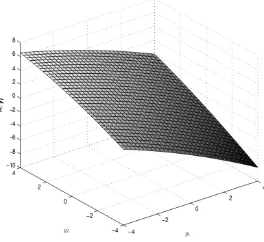
Two observations of Proposition 1 are very useful. First, the integrals Ii’s all involve
φ(y;0,Σ11) which is quite peaked around y= 0. Second, aroundy= 0, the exercise boundary
x(y) is quite close to being linear iny. Hence the same is true for the functionA(y). Figure 1
confirms this by giving a sample plot of A(y) when N = 2. The parameters used are the same
ones we use later for numerical comparisons in the three-asset case, and we fix K = 30 with
We now derive the approximations for the exercise boundary x(y) of the spread option and
the functionA(y) to second order in yaround y=0 as follows:
Proposition 3. The exercise boundary x(y) can be approximated to second order in y as
x(y)≈x(0) +∇x|′0y+1 2y
′∇2x| 0y,
where
x(0) = log(R+K)−µ0 ν0
,
(∇x|0)k =
eµkν
k
ν0(R+K)
, k= 1,2,· · ·, N,
(∇2x|0)i,j =−
νiνjeµi+µj
ν0(R+K)2
+δi,j
νj2eµj
ν0(R+K)
, i, j= 1,2,· · ·
with δi,j being the Kronecker delta function, and
R=
N
X
k=1
eµk.
Accordingly, the function A(y) can be approximated as
A(y) = µx|py−x(y)
Σx|y ≈
c+d′y+y′Ey,
where
c=−log(R+K)−µ0 ν0pΣx|y
, (13)
d= p1
Σx|y(Σ
−1
11Σ10− ∇x|0), (14)
E=− 1
2p
Σx|y(∇
2x
|0). (15)
Our goal is to use an approximation of A(y) in Proposition 1 so that we can perform the
integralsIk’s. For this purpose, we further expand Φ
³
c+d′y+y′Ey´into three terms to second order iny′Ey around y′Ey=ǫ, for some suitably chosenǫ. With the help of an identity in Li (2007), we are now able to perform the integration and obtain a closed-form approximation for
the spread option price as presented in Proposition 4. Proposition 4 is one of the most important
Proposition 4. Let K ≥ 0 and detΣ 6= 0. The spread option price Π under the general
jointly-normal returns setup is given by
Π =e−rT+µ0+12ν02 I
0−
N
X
k=1
e−rT+µk+12ν 2
k I
k−Ke−rT IN+1. (16)
The integralsIi’s are approximated as
Ii≈J0(ci,di) +J1(ci,di)−
1 2J
2(c
i,di), i= 0,1,· · ·, N + 1 (17)
where the scaler function Ji’s are defined as
J0(u,v) = Φ
µ
u
√
1 +v′v
, (18)
J1(u,v) =√ λ
1 +v′v·φ
µ
u
√
1 +v′v
, (19)
J2(u,v) = u
(1 +v′v)3/2 ·φ
µ
u
√
1 +v′v
(20)
n
λ2+ 2tr[(PFP)2]−4λ(1 +v′v)(v′P2FP2v) + (4u2−8−8v′v)kPFP2vk2o,
with
P=P(v)≡(I+vv′)−1/2, (21)
λ=λ(u,v)≡u2v′P2FP2v+tr(PFP)−tr(F), (22)
where tr stands for the trace operator of a matrix. The scalers ci, vectors di,and matrix Fare
given by
c0 =c+tr(F) +ν0
q
Σx|y+ν0Σ10′d+ν02Σ10′EΣ10, (23)
d0 =Σ
1 2
11(d+ 2ν0EΣ10), (24)
ck=c+tr(F) +νkek′Σ11d+νk2ek′Σ11EΣ11ek, k= 1,2,· · ·, N (25)
dk=Σ
1 2
11(d+ 2νkEΣ11ek), k= 1,2,· · ·, N (26)
cN+1 =c+tr(F), (27)
dN+1 =Σ
1 2
11d, (28)
F=Σ
1 2
11EΣ
1 2
11, (29)
Notice that we have used boldface subscriptiindito denote thei-th vector in order to avoid
confusion with thei-th component di of the vectord. As we see, the calculation of the spread
option price is quite straightforward in the second-order boundary approximation. A naive look at Proposition 4 might imply that we need to perform a lot of costly matrix multiplications.
However, Proposition 5 below shows that we only need to perform a very limit number of matrix
multiplications. The critical observation in obtaining Proposition 5 is thatv is an eigenvector
of P(v) defined in equation (21). The proof of Proposition 5 is in the Appendix.
Proposition 5. With P=P(v) as defined in equation (21), we have
P=I−θvv′, P2=I−ψvv′,
where the scalars θ and ψ are given by
θ=θ(v) =
√
1 +v′v−1
v′v√1 +v′v, ψ=ψ(v) =
1
1 +v′v. (30)
Furthermore, we have
tr[(PFP)2] =tr(F2)−ψ(1 +ψ)v′F2v, (31)
v′P2FP2v=ψ2v′Fv, (32)
kPFP2vk2 =ψ2£
v′F2v−ψ(v′Fv)2¤
, (33)
tr(PFP) =tr(F)−ψv′Fv. (34)
Thus the scaler function Ji’s given in (18) can be simplified as
J0(u,v) = Φ³upψ´, (35)
J1(u,v) =ψ32(ψu2−1)v′Fv·φ
³
upψ´, (36)
J2(u,v) =uψ32 ·φ
³
upψ´ n2tr(F2)−4(1−tr(F))(ψ−ψ2)v′Fv (37)
+ψ2(9 + (2−3u2)ψ−u2(4−u2)ψ2)(v′Fv)2−2ψ(5 + (1−2u2)ψ)v′F2vo.
Proposition 5 is very useful in the actual implementation of the second-order boundary
approximation because it reduces the calculation of the four computationally costly terms in
Proposition 4, tr[(PFP)2], v′P2FP2v, kPFP2vk2 and tr(PFP), to four much simpler expres-sions, namely,tr(F),tr(F2),v′Fv, andv′F2v. Our numerical analysis shows that Proposition 5 reduces the computational time of the second-order boundary approximation as presented in
Proposition 4 by about several hundred times. In the Appendix we comment more on the
implementation of the second-order boundary approximation.
C. Spread option Greeks and their approximation
Proposition 2 and Proposition 4 give approximations for multi-asset spread options prices. Below
we derive approximations for the important Greeks in our setup. Fast and accurate calculation
of these Greeks is very important because the Greeks are very useful in hedging, portfolio
rebalancing, risk assessment such as VaR calculations, among other things. There are many
approaches to calculating the Greeks, including finite difference method using Monte Carlo,
numerical integration, and more recently, Malliavin calculus. For multi-asset spread options,
especially when the number of assets is large, numerical methods often prove to be extremely slow to be applicable in practice. Thus a closed-form approximation is extremely useful. We use
the second-order boundary approximation in the computation of the Greeks because although
the extended Kirk approximation is fairly accurate for the prices, it does not give as accurate
Greeks as the second-order boundary approximation does.
We will focus on the most important Greeks, the deltas and kappa. Because the second-order
boundary approximation is extremely fast and accurate, Greeks other than the deltas and kappa
can be very efficiently computed using finite difference method.
To compute the deltas and kappa, we need to know the dependence ofµk’s and νk’s on the
initial asset prices sk’s and the strike priceK. We will assume that for each k,µk is a function
ofsk while νk is independent ofsk. This is not very restrictive because both the two important
special cases of our general setup, namely, the GBMs case and the log-OU case, satisfy this
requirement.
Now let us define the price vector
S= (e−rT+µ0+21ν20,−e−rT+µ1+12ν12,· · · ,−e−rT+µN+12ν 2
N,−Ke−rT)′.
Notice that in the GBMs case, equation (5) holds so
S= (s0e−q0T,−s1e−q1T,· · ·,−sNe−qNT,−Ke−rT). (38)
In the log-OU case, equation (7) gives us that fork= 0,1,· · · , N,
Sk= exp
³
−rT +ηk(1−e−λkT) +e−λkT logsk−
σ2
k
4λk
¡
1−e−λkT¢2 ´
. (39)
From Proposition 1 and 4 , we have the following result for the deltas and kappa. The proof
Proposition 6. Let K≥0. Suppose that in the general jointly normal returns setup,µk is only
a function of sk while νk is independent of sk for each k= 1,· · · , N. Then
∆0 ≡
∂Π ∂s0
= ∂µ0 ∂s0
S0I0, (40)
∆k≡
∂Π ∂sk
=−∂µk ∂sk
SkIk, k= 1,2,· · ·, N (41)
κ≡ ∂Π ∂K =−e
−rTI
N+1. (42)
In particular, in the geometric Brownian motions case, we have
∆0 =e−q0TI0, ∆k =−e−qkTIk, k= 1,2,· · · , N.
In the log-Ornstein-Uhlenbeck case, withSk’s given in equation (39), we have
∆0 =
e−λ0T s0
S0I0, ∆k=−
e−λkT
sk
SkIk, k= 1,2,· · · , N.
The vector I={Ik} can then be approximated by Proposition 4.
Proposition 6 shows that Proposition 4 is not only useful for computing spread option prices,
but also useful for computing the deltas and kappa of the spread option. In particular, if
Proposition 4 is implemented with the vectorization technique, then the computation of the
vectorIsimultaneously gives us all the deltas and kappa. This is not the case if one uses Monte
Carlo simulation to compute the prices and then uses finite difference to approximate the Greeks.
D. Extension to hybrid spread-basket option prices
We now extend both the extended Kirk approximation and the second-order boundary
approx-imation to a generic hybrid spread-basket option with time-T payoff
hXM
i=1
wiSi(T)− M+N
X
j=M+1
wjSj(T)−K
i+
,
where K, wi’s are positive constants. Again, we assume that conditioning on the initial asset
prices, logSi(T) are jointly normally distributed with mean µi, variance νi2, and correlation
matrix ρi,j for i, j = 1,2,· · · , M +N. Without loss of generality, we will assume that all
wi equal 1 as the weights wi can be easily absorbed by defining Si′ = wiSi and noticing that
µ′i = logwi+µi, νi′ =νi and ρ′i,j =ρi,j. In addition, we allow one ofSi (i= 1,· · · , M) to be a
constant, thus effectively allowingK to be negative. Except for the possibility of a constantSi
To compute the price of this hybrid spread-basket option, we again utilize the well-known
technique in pricing Asian options. Specifically, let
H0(t)≡
M
X
i=1
Si(t), and Hk(t)≡Sk+M(t) k= 1,2,· · ·, N.
Notice that the final payoff of the hybrid option now formally reduces to that of a standard
spread option
h
H0(T)−
N
X
k=1
Hk(T)−K
i+
.
However, theHi’s are no longer jointly normally distributed, nor isH0(T) normally distributed.
The idea is to approximate the distribution of H0(T) by the corresponding geometric average
of theSi’s. In addition, in order to apply Proposition 4, we need the correlation matrix of the
Hi’s. The detailed procedure is as follows.
Define random variables X and Yk’s by
X= logH0(T)−µ
H
0
ν0H , Yk=
logHk(T)−µHk
νkH , k= 1,2,· · · , N
withµH
k =µk+M and νkH =νk+M fork= 1,· · · , N, and
µH0 = log¡
M
X
i=0
eµi+12ν 2
i¢−1
2(ν
H
0 )2, ν0H =
1 M v u u t M X i=1 M X j=1
ρi,jνiνj.
Then X and the Yi’s can be approximated as jointly normally distributed with mean vector0,
variance vector1, and correlation matrixΣ= (̺i,j), i, j = 0,1,· · ·, N, where
̺0,0 = 1,
̺0,k =̺k,0 =
1 M νH
0
³XM
i=1
ρi,kνi
´
, k= 1,2,· · · , N
̺i,j =ρM+i,M+j, i, j= 1,2,· · ·, N.
The above equations can be proven in a very similar way to Proposition 2. Notice that under
the GBMs case, the quantityµH0 are usually further approximated as
µH0 = logH(0) +³rT − 1 M
M
X
i=1
qiT+
1 2M
M
X
i=1
νi2´.
Once we have approximated the Hi’s using the jointly normal setup, we can use either the
extended Kirk approximation in Proposition 2 or the second-order boundary approximation in
IV. Comparison of accuracy and speed with existing methods
A. Existing pricing methods
When the number of assets is small, numerical integration method can be used to calculate
spread option prices by using Proposition 1. Although very accurate, it is not quite applicable
for multi-asset spread options when the number of assets is large because of the huge computation
cost. The same is true for partial differential equation technique. Another widely used numerical
method is Monte Carlo simulation. The advantage of Monte Carlo simulation is that it is very
flexible and is able to value spread options under many different distributional assumptions. The
shortcomings are that the results are not always accurate enough, even after variance reduction
techniques such as antithetic method, control variate and importance sampling are applied.
Also, the Greeks need to be calculated with extra effort, usually by approximating them using finite difference. The biggest shortcoming is that Monte Carlo simulation is generally very
time-consuming, especially when the dimension is high and the number of option prices need to be
computed is large.
Given the high computational cost of numerical methods for multi-asset spread option, it is
extremely useful to design approximation techniques. However, until very recently, not much
work has been done on this subject. Carmona and Durrleman (2005) propose approximate
formulas for the lower and upper bounds of multi-asset spread options by solving a nonlinear
optimization problem. They only consider the geometric Brownian motions case. The lower
bound is quite accurate while the upper bound is less accurate. Therefore we just compare our
method with their lower bound. We give a brief description of the Carmona and Durrleman method below. Interpreting σN+1 = 0 and letting C = Σ⊕1, the lower bound of the spread
option price is given as follows.
Π =
N+1
X
i=0 SiΦ
³
d∗+ (C12z∗)
iσi
√
T´,
where the scalerd∗ and unit length vectorz∗ satisfy the following system of nonlinear equations
N+1
X
i=0 Siσi
√
T(C12)
ij φ
³
d∗+ (C12z∗)
iσi
√
T´−µz∗j = 0, for j= 0,· · ·, N + 1 (43)
N+1
X
i=0 Si φ
³
d∗+ (C12z∗)iσi√T
´
= 0, (44)
addition, like our second-order boundary approximation, Carmona and Durrleman’s method also
requires the somewhat expensive calculation of the square root of Σ. Interpreting sN+1 ≡ K,
the deltas and kappa are given by
∂Π ∂si
= Si si ·
Φ³d∗+ (C12z∗)
iσi
√
T´, i= 0,1,· · ·, N + 1. (45)
One very nice feature about this method is that it always gives a lower bound for the actual
price. The main difficulty of applying Carmona and Durrleman’s method is in solving the system
of nonlinear equations, because there is not much guidance on the choice of initial values ford∗,
z∗ and µ.
B. Numerical performance
We now compare our methods, namely, the extended Kirk approximation and the second-order
boundary approximation, with Monte Carlo simulation, numerical integration method based on
Proposition 1, and Carmona and Durrleman’s method. We perform the comparisons for four different dimensionsN+1, namely, 3,20,50, and 150 using an artificial correlation matrix similar
to the one used in Carmona and Durrleman (2005). In addition, in order to test various methods
using a more plausible correlation matrix, we also apply the methods to two hypothetical spread
options. One is between the S&P 500 index and the 30 component stocks of the Dow Jones
Industrial Average (DJIA) index and the other is between the S&P SmallCap 600 index and the
DJIA components. All methods are implemented in MATLAB 7.0 on a Dell Optiplex GX620
with 3.80 GHz Intel Pentium(R) 4 CPU and 3G RAM. For the purpose of definiteness and the
fact that Carmona and Durrleman (2005) only consider the geometric Brownian motions case,
we will only compare models in this special case.
For the Monte Carlo simulation, we generate 10,000,000 replicates. We use Proposition 1 rather than equation (10) because if one uses equation (10), then the information on the random
variablesxandyis completely lost if the option happens to be out of money. The use of
Propo-sition 1 amounts to an importance sampling technique. In the actual implementation we find
that it gives very large variance reduction in Π. The numerical integration method is only used
for the 3-dimension case because the computational cost is exceedingly high when the dimension
is high. The numerical integration results computed with error tolerance level 10−8 are used as actual option prices to calculate the relative pricing errors (ΠApproximation−ΠActual)/ΠActual. For
Carmona and Durrleman’s method, we use the globally convergent Newton-Raphson method as
optimal solution. However, the optimization is still extremely sensitive to the choice of initial
values and very often fails. The region of initial values that will lead to solutions is an unknown
function of the parameters of the spread option, namely, µi,νi and Σ, and Carmona and
Dur-rleman (2005) does not give much guidance on how to choose the initial values. Because of this,
extensive numerical experiments are often needed to find out the appropriate initial values for
different options, which can take from one minute to as long as half an hour. We thus conclude
that some guidance on how to choose the initial values in Carmona and Durrleman’s method is
crucial for the method to be useful in large scale real-life computations.
Spread options on 3 assets.
As a first example, we consider spread options on 3 assets. We set T = 0.25, r = 5%, and the
dividend rate zero. The initial asset prices are s0 = 150, s1 = 60, and s2 = 50. The volatilities
of all three assets are given by the same σ and we vary σ to be 0.3 and 0.5. We varyK to be
from 30 to 50 with increment 5. The correlation matrix for the asset returns is given by
Σ=
1 0.2 0.8 0.2 1 0.4 0.8 0.4 1
.
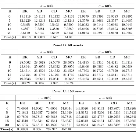
Table 1 reports the prices for each of the five methods we compare together with the average
computing times. The numerical integration results are used as the actual prices. Looking
at the relative errors, both our methods are quite accurate with the second-order boundary
approximation being more accurate than the extended Kirk approximation. In particular, the
relative pricing error of the extended Kirk approximation is in the order of 10−2, while that of the second-order boundary approximation is in the order of 10−5. Monte Carlo simulation with 10,000,000 replications and the use of Proposition 1 gives quite accurate results, but usually
still not as accurate as the second-order boundary approximation. Carmona and Durrleman’s method is also quite accurate but not as good as our second-order boundary approximation.
Furthermore, in the actual implementation we need to spend about 20 minutes to find good
starting values for the nonlinear equations that one has to solve in their method. Even if good
starting values are found, their method is still slower than both our methods. The average
computing times for both our methods are in the order of 10−3second, while both the numerical integration and Monte Carlo simulation methods take considerably more time.
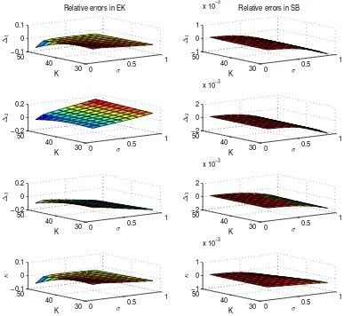
Table 2 lists the results for four important Greeks for all the methods, namely, the three
deltas and the kappa. Here we fixK = 30. Again, the qualitative conclusions are the same for
Greeks between the extended Kirk approximation and the second-order boundary
approxima-tion. Parameters are still the same, but now with K varies in the range [30,50] and σ varies
in the range [0.1,0.9]. The actual values for the Greeks are computed using numerical integra-tion. The Greeks for the extended Kirk approximation are obtained by differentiating equation
(11) in Proposition 2. The Greeks for the second-order boundary approximation are given in
Proposition 6. The Greeks for Carmona and Durrleman’s method is given in equation (45).
Figure 2 indicates that for the purpose of calculating the Greeks, the second-order boundary
approximation should be preferred to the extended Kirk approximation.
Spread options on 20, 50 and 150 assets.
Next, we consider spread options on multiple assets with numbers of assetsN + 1 equal 20, 50
and 150, respectively. We will consider symmetric target assets with initial pricess0 = 10(N+1)
and s1 =· · · =sN = 10. We set T = 0.25, r = 5%, and dividend rate zero. The correlation
matrix is set to be
Σ=
1 ρ · · · ρ
ρ 1 . .. ... ..
. ... . .. ρ ρ · · · ρ 1
(46)
withρ= 0.4. All assets returns have the same volatilityσ and we varyσto be either 0.3 or 0.6. We vary K from 0 to 20 with increment 5.
Table 3 reports the prices of spread options with different number of assets, different
volatil-ities σ and strikes K for each of the four methods we consider, together with the average
computing time of each method. The results for different dimensionN+ 1 are reported in three
different panels. SinceN is large, numerical integration is no longer feasible so we do not know
the exact actual option prices and as a result, we do not know the exact relative pricing errors.
However, the results from Monte Carlo simulation can serve as a rough comparison benchmark.
The results indicate that when the target assets are more symmetric, the extended Kirk
approx-imation is more accurate. Again, both our methods are among the fastest and the second-order
boundary approximation is much more accurate than the extended Kirk approximation and Carmona and Durrleman’s method.
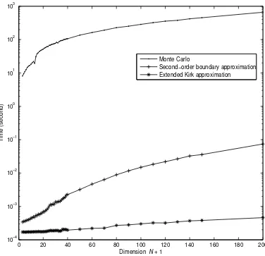
Figure 3 gives the computing time as a function of dimensionsN+ 1. The horizontal axis is
dimensionN+ 1, which we vary from 3 to 200. The vertical axis is time in log scale. We do not
plot the computing times for Carmona and Durrleman’s method because it often takes more than
20 minutes to search for good initial starting values for their algorithm. If we do not include
lie somewhere between the second-order boundary approximation and Monte Carlo simulation.
As we see, up to dimension 25, both our methods take less than 10−3 second to compute the price of one spread option. The extended Kirk approximation remains within 10−3 second for all dimensions, while the second order boundary approximation remains within 10−1 second.
Monte Carlo simulation takes considerable more time, ranging from 8 seconds in dimension 3
to over 500 seconds in dimension 200. For all dimensions, the computing times in the extended
Kirk approximation are about 0.001% or 0.0001% of those in Monte Carlo simulation while
the computing times in the second-order boundary approximation are about 0.01% of those in
Monte Carlo simulation.
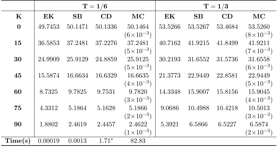
Spread options on two S&P indices and DJIA components.
Our final numerical example considers two hypothetical spread options. The first one is written on the S&P 500 index and the 30 component stocks of the Dow Jones Industrial Average (DJIA)
index. The second one is written on the S&P SmallCap 600 index and DJIA components.
Both options are very interesting in practice because industrial practitioners pay very close and
constant attention to the different performance among large company stocks, small company
stocks and the whole market. For our numerical experiments, these options are very interesting
because now the target assets are not completely symmetric.
For the first spread options, the final payoff is given by£
S0(T)−Pk30=1Sk(T)−K
¤+
, where
S0 is chosen to be the S&P 500 index multiplied by 1.15, andS1,· · · , S30the prices of the DJIA
component stocks. The weight 1.15 is chosen such that the spread option is near the money.
Because of occasional additions and deletions of the DJIA components, the DJIA component stocks are fixed as those on August 29th, 2007. For the second spread option, S0 is chosen to
be the S&P SmallCap 600 index multiplied by 4.
We consider two different maturities, T = 1/6 andT = 1/3. For each maturityT, to obtain
µk and νk, we use equation (2) and compute the mean and variance of the historical T-period
returns Rk,T. For the first option, we use historical daily price data from the CRSP (Center
for Research in Security Prices) data base from July 9th, 1986 to August 29th, 2007 because
the stock prices for several companies are only available after July 9th, 1986. The returns
are calculated using daily close prices after adjusting for stock splits. The prices on August
29th, 2007 are used to determine the initial asset prices sk’s. Alternatively, we could have used
equations (5) to computeµk’s andνk’s by estimating the dividend rates. The correlation matrix
Σ is estimated from the historical correlation matrix of the Rk,T’s. For the second option, we
SmallCap 600 index is only available after August 16th, 1995. To include both in-the-money
and out-of-the-money options, we vary K from 0 to 75 with increment 15 for the first option,
and varyK from 0 to 120 with increment 30 for the second one.
Table 4 and Table 5 report the prices of the two spread option with different maturities T
and strikesK, together with the average computing time of each method. Because actual prices
are not available, we use the results from the Monte Carlo simulation as a rough benchmark. As
we see, the extended Kirk approximation in this nonsymmetric case becomes less accurate, with
relative pricing error sometimes quite significant. Our second-order boundary approximation
give more accurate approximation for the option prices than Carmona and Durrleman’s method.
V. Conclusion
In this paper, we study spread options written on multiple assets. We develop two closed-form approximations for pricing them, namely, the extended Kirk approximation and the
second-order boundary approximation. Numerical analysis demonstrates that both our methods are
very robust, fast and accurate, with the second-order approximation being more accurate than
the extended Kirk approximation and Carmona and Durrleman’s method. For spread options
written on 3 assets, the relative pricing error of the second-order approximation is in the order
of 10−4 with an average computing time for each option of 2×10⁻⁴. For dimensions up to about 100, the second-order boundary approximation takes less than 10−2 second. Thus, our method enables the accurate pricing of a bulk volume of spread options on multiple assets with different
contract specifications in real time, which offer traders a potential edge in financial markets. We
also extend our results to hybrid spread-basket options.
In addition, our approximations, especially the second-order boundary approximation, can
be used to approximate the Greeks of spread options, which serve as valuable tools in
finan-cial applications such as calculating the delta-hedging position of a portfolio containing spread
options.
There are a few directions that one can take to extend and improve the results in this paper.
First, in the geometric Brownian motions case, our results can be easily extended to incorporate
jumps in the price processes of the assets. Second, the boundary approximation idea might be
Appendix
A. Proofs
Proof of Proposition 1:
The conditional density of X given Y =y is φ(x;µx|y,Σx|y). By formula for the determinants for partitioned matrix, we have Σx|y6= 0 since
detΣ= det(Σ11−Σ10Σ′10) = (det(Σ11))−1Σx|y6= 0.
Thus, we can compute the price of the spread option as follows:
Π =e−rT
Z
RN Z
R ³
eν0x+µ0
−
N
X
k=1
eνkyk+µk−K ´+
φ({x,y};0,Σ)dxdy
=e−rT
Z
RN
φ(y;0,Σ11)dy
Z ∞
x(y)
Ã
eν0x+µ0
−
N
X
k=1
eνkyk+µk−K !
φ(x;µx|y,Σx|y)dx.
By virtue of the identity
Z ∞
x0
etxn(x;µ, σ2)dx=eµt+σ2t2/2Φ
µ
µ−x0
σ +σt
, (47)
the inner integral can be performed to yield
Π = e12ν 2
0Σx|y+µ0−rT
Z
RN
eν0µx|y φ(y;0,Σ
11) Φ ³
A(y) +ν0
q
Σx|y ´ dy − N X k=1
e−rT
Z
RN
eνkyk+µk φ(y;0,Σ 11) Φ
³
A(y)´dy
−Ke−rT
Z
RN
φ(y;0,Σ11) Φ ³
A(y)´dy. (48)
Completing the square after a change of variablez=y−ν0Σ10 gives
e12ν 2
0Σx|y+µ0−rT
Z
RN
eν0µx|y φ(y;0,Σ
11) Φ ³
A(y) +ν0
q
Σx|y ´
dy
=e−rT+µ0+12ν02
Z
RN
φ(z;0,Σ11)Φ ³
A(z+ν0Σ10) +ν0
q
Σx|y ´
dz.
Similarly, a change of variable z=y−νkΣ11ek, fork= 1,2,· · ·, N, gives
e−rT
Z
RN
eνkyk+µk φ(y;0,Σ 11) Φ
³
A(y)´dy
=e−rT+µk+12ν 2
k Z
RN
φ(z;0,Σ11)Φ ³
A(z+νkΣ11ek) ´
Collecting terms, we get the expressions in Proposition 1.
Proof of Proposition 2:
Consider a spread option on two assets with final payoff (S0(T)−L(T)−K)+, where logS0(T)
and logL(T) are jointly normal with means µ0,µa, variances ν02,νa2, and correlationρa. Then
the two-asset Kirk approximation for the spread option price is given by
eµ0+12ν02−rTΦ(d
1)−(eµa+
1 2ν
2
a−rT +Ke−rT)Φ(d 2),
where
d1 =
1 νK
log³ e
µ0+12ν02−rT eµa+12νa2−rT +Ke−rT
´
+1
2νK, d2=d1−νK,
with
νK =
q
ν02+m2ν2
a−2mρaν0νa and m=
eµa+12ν 2
a−rT
eµa+12ν 2
a−rT +Ke−rT
.
To apply the above result for multi-asset spread options with payoff (S0(T)−PNk=1SN(T)−K)+,
we let L(T) = PN
k=1Sk(T). A common technique is to approximate the arithmetic average
PN
k=1Sk(T)/N by the geometric averageQNk=1Sk(T)1/N.
For νa, notice that
νa2= Var(logL(T))≈Var³log¡
N
N
Y
k=1
Sk(T)1/N
¢´
= Var³1 N
N
X
k=1
logSk(T)
´ = 1 N2 N X i=1 N X j=1
ρi,jνiνj.
For ρa, notice that
ρa=
1 ν0νa
Cov(logS0(T),logL(T))≈
1 ν0νa
Cov³logS0(T),log
N
Y
k=1
Sk(T)
1
N
´
= 1 ν0νa
Cov³logS0(T),
1 N
N
X
k=1
logSk(T)
´
= 1 N νa
N
X
k=1
ρ0,kνk.
To compute µa, notice that since logL(T) is approximated normally distributed with mean
µa and varianceνa2, we have EelogL(T) ≈eµa+ν
2
a/2. Thus,
µa≈logEelogL(T)−
1 2ν
2
a= logE N
X
k=1
Sk(T)−
1 2ν
2
a = log
³XN
k=1
eµk+ νk2
2
´
The final step of the proof involves simplifying the expressions for m and m0 using the
expression for µa.
Proof of Proposition 3:
This proposition follows directly from Taylor expanding the exercise boundary (9) to second
order in y aroundy=0:
(∇x|0)k=
∂x ∂yk ¯ ¯ ¯ ¯ 0 = e
µkν
k
ν0(R+K)
, k= 1,2,· · · , N
(∇2x|0)i,j =
∂2x ∂yi∂yj
¯ ¯ ¯ ¯ 0
=− νiνje
µi+µj
ν0(R+K)2
+δi,j
νj2eµj
ν0(R+K)
, i, j= 1,2,· · · , N.
Proof of Proposition 4:
From Proposition 1, we have
Π =e−rT+µ0+12ν02 I
0−
N
X
k=1
e−rT+µk+12ν 2
k I
k−Ke−rT IN+1.
First, by Proposition 3,A(y)≈c+d′y+y′Ey.Next, we treaty′Eyas an independent quantity from c+d′y and expand Φ(A(y))≈Φ¡
c+d′y+y′Ey¢
to second order in y′Ey around
y′Ey=ǫ=
Z
RN
φ(y;0,Σ11)y′Eydy=tr(F).
Since
dΦ¡
c+d′y+y′Ey¢
dy′Ey
¯ ¯ ¯ ¯
y′Ey=ǫ
=φ(c+ǫ+d′y),
d2Φ¡
c+d′y+y′Ey¢
d(y′Ey)2
¯ ¯ ¯ ¯
y′Ey=ǫ
=−(c+ǫ+d′y) φ(c+ǫ+d′y),
we have
IN+1 =
Z
RN
φ(y;0,Σ11)Φ ¡
A(y)¢
dy (49)
≈
Z
RN
φ(y;0,Σ11)Φ ¡
c+d′y+y′Ey¢
dy (50)
≈
Z
RN
φ(y;0,Σ11) h
Φ¡
c+ǫ+d′y¢
+φ(c+ǫ+d′y)(y′Ey−ǫ) (51)
−1
2(c+ǫ+d
′y) φ(c+ǫ+d′y)(y′Ey−ǫ)2idy (52)
≡J0N+1+J1N+1−1
2J
2
where
J0N+1 =
Z
RN
φ(y;0,Σ11)Φ ¡
c+ǫ+d′y¢
dy,
J1N+1 =
Z
RN
φ(y;0,Σ11) φ(c+ǫ+d′y) (y′Ey−ǫ)dy,
J2N+1 =
Z
RN
φ(y;0,Σ11)(c+ǫ+d′y) φ(c+ǫ+d′y)(y′Ey−ǫ)2dy.
ForJ0N+1, a change of variable w=d′ygives
J0N+1=
Z
R
φ(w; 0,d′Σ11d)Φ ¡
c+ǫ+w¢
dw. (54)
The following result in Li (2007) is very useful and we refer readers to Li (2007) for a proof:
Z ∞
−∞
Φ(a+by)φ(y;µ, σ2) dy= Φ
µ
a+bµ
√
1 +b2σ2
.
With the help of the above identity, the integral in (54) can be performed to give
J0N+1 = Φ³√ c+ǫ
1 +d′Σ11d
´
= Φ
µ
cN+1
q
1 +d′
N+1dN+1 
=J0(cN+1,dN+1). (55)
ForJ1N+1, a change of variable z=Σ−
1 2
11y gives
J1N+1 =
Z
RN
φ(z;0,I) φ(c+ǫ+d′N+1z) (z′Fz−ǫ)dz (56)
=
Z
RN
φ(z;0,I) φ(c+ǫ+d′N+1z) (z′Fz)dz−
ǫ
q
1 +d′N+1dN+1
φ³q cN+1
1 +d′N+1dN+1
´
.
(57)
We now perform a second change of variable z=a+Pw, where
P= (I+dN+1d′N+1)−1/2, a=−(c+ǫ)P2dN+1.
This choice of Pand agives
(c+ǫ+d′N+1z)2+|z|2 =|w|2.
The determinant of the Jacobian is given by
det ¯ ¯ ¯ ¯ dz dw ¯ ¯ ¯ ¯
where we have used Schur’s formula: det(I+dN+1d′N+1) = 1 +d′N+1dN+1. Completing the
square in equation (56), we can simplify J1N+1 to
J1N+1=
φ³√1+d′ c
N+1dN+1
´
q
1 +d′
N+1dN+1 µ Z
RN
φ(w;0,I) (a+Pw)′F(a+Pw)dw−ǫ
.
LetW be a random variable with density φ(w;0,I), then
E[Wi] = 0, E[WiWj] =δi,j, E[WiWjWk] = 0,
E[WiWjWkWl] =δi,jδk,l+δi,kδj,l+δi,lδj,k, E[WiWjWkWlWm] = 0.
Thus, withλgiven in the text, we have
E(a+PW)′F(a+PW)−tr(F) =λ=λ(cN+1,dN+1),
and
J1N+1 = qλ(cN+1,dN+1)
1 +d′
N+1dN+1
φ³q cN+1
1 +d′
N+1dN+1 ´
=J1(cN+1,dN+1).
ForJ2
N+1, similar changes of variable give
J2N+1 =
φ³√ cN+1
1+d′
N+1dN+1
´
q
1 +d′N+1dN+1
n
ǫ2E£
c+ǫ+d′N+1(a+PW)
¤
−2ǫE£(c+ǫ+d′N+1(a+PW))((a+PW)′F(a+PW))
¤
+E£
(c+ǫ+d′N+1(a+PW))((a+PW)′F(a+PW))2
¤o
.
After tedious calculations of the above expectation, we get thatJ2N+1 =J2(cN+1,dN+1) as in
Proposition 4.
For I0, notice that
I0=
Z
RN
φ(y;0,Σ11)Φ ³
A(y+ν0Σ10) +ν0
q
Σx|y´dy
≈
Z
RN
φ(y;0,Σ11)Φ ³
(c+ǫ+ν0
q
Σx|y) +d′(y+ν0Σ10) + (y+ν0Σ10)′E(y+ν0Σ10) ´
dy
=
Z
RN
φ(y;0,Σ11)Φ ¡
c0+d′0y+y′Ey ¢
dy.
Comparing the last equation with equation (50), we immediately get without any calculations
that
I0≈J0(c0,d0) +J1(c0,d0)−
1 2J
Similarly, we get
Ik =
Z
RN
φ(y;0,Σ11)Φ ³
A(y+νkΣ11ek) ´
dy
≈
Z
RN
φ(y;0,Σ11)Φ ³
c+ǫ+d′(y+νkΣ11ek) + (y+νkΣ11ek)′E(y+νkΣ11ek) ´
dy
=
Z
RN
φ(y;0,Σ11)Φ ¡
ck+d′ky+y′Ey
¢
dy
≈J0(ck,dk) +J1(ck,dk)−
1 2J
2(c
k,dk).
Proof of Proposition 5:
By the definition ofP,
P2 = (I+vv′)−1 =I−ψvv′,
where the last equality follows from the so-called updating formula (see, for example, Greene
2000). To see thatI−θvv′ is the unique square root ofP2, notice that I−θvv′ is symmetric, and 2θ−θ2v′v=ψ, so
(I−θvv′)2 =I−(2θ−θ2v′v)vv′ =I−ψvv′.
The other equations now follow from brute-force computations.
Proof of Proposition 6:
Notice that
Π =e−rT
Z
RN
φ(y;0,Σ11)dy
Z ∞
x(y)
³
eν0x+µ0
−
N
X
k=1
eνkyk+µk−K ´
φ(x;µx|y,Σx|y)dx.
Thus,
∂Π ∂s0
= e−rT∂µ0 ∂s0
Z
RN
φ(y;0,Σ11)dy
Z ∞
x(y)
eν0x+µ0φ(x;µ
x|y,Σx|y)dx
−e−rT
Z
RN
φ(y;0,Σ11) ³
eν0x(y)+µ0
−
N
X
k=1
eνkyk+µk−K
´∂x(y)
∂s0
φ(x(y);µx|y,Σx|y)dy
= ∂µ0 ∂s0
S0I0.
The other deltas and kappa can be proven similarly. The two special cases can be obtained by
B. Implementation of the second-order boundary approximation
While it is very straightforward to implement the second-order boundary approximation, an
efficient implementation which minimizes the computing time requires some effort. Below we
comment on some of the details of the actual implementation along with some useful tricks:
1. Σ−111Σ10. Matrix inversion is a costly operation and should be avoided. Instead, we use
matrix division to find the solutionzofΣ10=Σ11z. BecauseΣ11is positive definite and
symmetric, Cholesky factorization is useful in solving the linear system. Alternatively, one
could use Gaussian elimination. The quantityΣ−111Σ10 is referred to in the computation
of Σx|y,d and many other places.
2. Σ12
11. Notice that sinceΣ11is positively definite and symmetric, an efficient algorithm to
compute its square root is through the similarity transformationΣ11=Q′ΛQ, whereQ
contains all the eigenvectors ofΣ11 and Λ is a diagonal matrix containing all the
corre-sponding eigenvalues. Then the square root ofΣ11 is given byΣ
1 2
11 =Q′Λ
1
2Q. Efficient
algorithm for performing similarity transformation of a positive definite and symmetric
matrix exists.
3. tr(F2). Once the matrixF is computed from equation (29), we can avoid computingF2
by computingtr(F2) as follows:
tr(F2) =
N
X
i=1
N
X
j=1
£
Fij¤2.
The right-hand-side can be computed very efficiently by first taking the element-by-element
square ofF and then taking the sum of all the elements. This is computationally more efficient than computing the matrixF2 because the former involvesN2 multiplications of
two real numbers while the latter involvesN3 multiplications.
4. v′v,v′Fv and v′F2v. Define a (N+ 2)×N matrixD as follows
D= (d0,d1,· · · ,dN,dN+1)′.
Notice that we need to computev′v,v′Fv and v′F2v forv=di fori= 0,1,· · ·, N + 1.
We use the following identities to compute the vectorsv′v,v′Fvand v′F2v:
v′v= rowsum(D.2), (58)
v′Fv= diag(DFD′), (59)
v′F2v= rowsum((DF).2), (60)
where rowsum is the operator of taking the row sum of a matrix and A.2 stands for the
element-by-element square of a matrixA. Written out component-wise, we have
(di)′di=
N
X
j=1
¡
Dij¢2, (61)
(di)′Fdi= (DFD′)ii, (62)
(di)′F2di=
N
X
j=1
£
(DF)ij¤2. (63)
Equations (61), (62) and (63) can be seen easily by noticing thatF is symmetric.
5. Vectorization. It is very important to use vectorization technique in the actual
imple-mentation to avoid for-loops in the program and further improve the efficiency. This is
especially important whenN is large. All the scaler quantities involving v, such as ψ(v),
θ(v), v′v, v′Fv, v′F2v, tr[(PFP)2], v′P2FP2v, and kPFP2vk2 should be treated as (N+ 2)×1 vectors, where the index is onv ranging fromd0 todN+1. In particular, this
means that we should use equations (58), (59) and (60) instead of (61), (62) and (63).
Furthermore,λ(u,v), J0(u,v),J1(u,v) andJ2(u,v) should be treated as (N+ 2)×1
vec-tors whereu ranges fromc0 tocN+1 and v ranges from d0 todN+1. Equation (17) then
allows us to treatI as a (N + 2)×1 vector. In turn, the spread option price in equation
(16) is simply given by
Π =S0I0−
N
X
k=1
SkIk−Ke−rT IN+1 =S′I.
Despite its seemingly complexity, the second-order boundary approximation is very
straight-forward to implement and our code in MATLAB is only about 30 lines. The second-order
boundary approximation is also extremely fast and the computation of Σ
1 2
11 is actually where
more than half of the computing time is spent. For example, when N = 50, the second-order
boundary approximation needs less than 3×10⁻³ second to compute the price of one spread option and the computation ofΣ
1 2
References
Carmona, R., and V. Durrleman. “Pricing and hedging spread options.” SIAM Review, 45 (2003), 627-685.
Carmona, R., and V. Durrleman. “Generalizing the Black-Scholes formula to multivariate con-tigent claims.”Journal of Computational Finance, 9 (2005), 42-63.
Deng, S. J., B. Johnson, and A. Sogomonian. “Exotic electricity options and the valuation of electricity generation and transmission assets.”Decision Support Systems, 30 (2001), 383-392.
Deng, S. J, M. Li, and J. Zhou. “Closed-form approximations for spread option prices and Greeks.” available at SSRN:http://ssrn.com/abstract=952747, (2006).
Girma, P. B., and A. S. Paulson. “Risk arbitrage opportunities in petroleum futures spreads.”
Journal of Futures Markets, 18 (1999), 931-955.
Greene, W. H.Econometric Analysis, Prentice Hall, New Jersey (2000).
Jarrow, R., and A. Rudd. “Approximate option valuation for arbitrary stochastic processes.”
Journal of Financial Economics, 10 (1982), 347-369.
Johnson, S. A., and Y. S. Tian. “Indexed executive stock options.”Journal of Financial Eco-nomics, 57 (2000), 35-64.
Johnson, R. L., C. R. Zulauf, S. H. Irwin, and M. E. Gerlow. “The soy-bean complex spread: An examination of Market Efficiency from the viewpoint of a production process.”Journal of Futures Markets, 11 (1991), 25-37.
Kirk, E.“Correlations in the energy markets.” InManaging Energy Price Risk. Risk Publications and Enron, London (1995), 71-78.
Li, M. “The impact of return nonnormality on exchange options.”Journal of Futures Markets, working paper, forthcoming, (2007).
Margrabe, W. “The value of an option to exchange one asset for another.”Journal of Finance, 33 (1978), 177-186.
Mbafeno, A. “Co-movement term structure and the valuation of energy spread options.” In
Mathematics of Derivative Securities. M. Dempster and S. Pliska, eds. Cambridge Univer-sity Press, Cambridge, UK (1997).
Routledge, S., D. J. Seppi, and C. S. Spatt. “The “Spark Spread”: An Equilibrium Model of Cross-Commodity Price Relationship in Electricity.” working paper. Carnegie Mellon University, (2001).
Pearson, N. “An efficient approach for pricing spread options.” Journal of Derivatives, Fall (1995), 76-91.
Shimko, D. “Options on futures spreads: Hedging, speculation, and valuation.” Journal of Futures Markets, 14 (1994), 183-213.
Wilcox, D. Energy futures and options: Spread options in energy markets. Goldman Sachs & Co., New York (1990).
−4
−2
0
2
4
−4 −2
0 2
4 −10 −8 −6 −4 −2 0 2 4 6 8
y1 y2
A(
[image:33.612.104.489.117.471.2]y)
Figure 1. The functionA(y) neary=0. Notice thatA(y) is approximately linear inyaround
0 0.5 1 30 40 50 −0.1 0 0.1 σ
Relative errors in EK
K ∆ 1 0 0.5 1 30 40 50 −1 0 1
x 10−3
σ
Relative errors in SB
K ∆ 1 0 0.5 1 30 40 50 −0.2 0 0.2 σ K ∆ 2 0 0.5 1 30 40 50 −2 0 2
x 10−3
σ K ∆ 2 0 0.5 1 30 40 50 −0.2 0 0.2 σ K ∆ 3 0 0.5 1 30 40 50 −2 0 2
x 10−3
σ K ∆ 3 0 0.5 1 30 40 50 −0.1 0 0.1 σ K κ 0 0.5 1 30 40 50 −1 0 1
x 10−3
σ
K
[image:34.612.102.489.107.463.2]κ
0 20 40 60 80 100 120 140 160 180 200 10−4
10−3 10−2 10−1 100 101 102 103
Dimension N + 1
Time (second)
Monte Carlo
[image:35.612.107.483.106.469.2]Second−order boundary approximation Extended Kirk approximation