http://dx.doi.org/10.4236/wjm.2014.42005
Non-Destructive Testing of Rods Using a Potential
Component of a Magnetic Field
A. K. Tomilin1, E. V. Prokopenko2 1
National Research Tomsk Polytechnic University, Tomsk, Russian Federation 2
D. Serikbayev East Kazakhstan State Technical University, Ust-Kamenogorsk, Republic of Kazakhstan Email: [email protected], [email protected]
Received November 6,2013; revised December 2, 2013; accepted January 1, 2014
Copyright © 2014 A. K. Tomilin, E. V. Prokopenko. This is an open access article distributed under the Creative Commons Attribu-tion License, which permits unrestricted use, distribuAttribu-tion, and reproducAttribu-tion in any medium, provided the original work is properly cited. In accordance of the Creative Commons Attribution License all Copyrights © 2014 are reserved for SCIRP and the owner of the intellectual property A. K. Tomilin, E. V. Prokopenko. All Copyright © 2014 are guarded by law and by SCIRP as a guardian.
ABSTRACT
An essentially new method for non-destructive testing of elastic electrically conductive rods using non-vortex electromagnetic induction is proved theoretically. An experimental technique for defining a location of a cross crack is offered.
KEYWORDS
Elastic Oscillation; Electric Mechanical Systems; Non-Destructive Testing; A Magnetic Field
1. Introduction
Developing efficient and highly precise methods for di- agnosing products is a relevant science task: non-de- structive testing allows defining timely defects of ele- ments of important constructions. There are several me- thods of non-destructive testing: magnetic-particle, ed- dy-current, liquid penetrant, acoustic, optical, radiation [1,2]. The Shock Pulse Method is widely applied [3], which is based on using the connection between natural frequencies of elastic oscillation and physical mechanical properties of materials and products. At the same time, piezoelectric accelerometers are used for transforming mechanical oscillation into electric signals. It is well known that their applying has some difficulties: signal filtration depends on frequency response of an accelero-meter and the way it is set up [3].
The authors from Kazan [4] considered the opportuni-ty of applying an ultrasonic method to the diagnosis of rods in their work. A way to define a rode defect by ana-lyzing the spectrum of fundamental frequencies is of-fered. The analysis implies comparing the oscillation spectrums of a defective product with ones defect free.
Akhtyamov A.M. and Karimov A. R. [5] offered a method allowing defining the location of a crack in a rod by natural frequencies of longitudinal oscillation in their article. Cracks are a kind of springs. At the same time, a
construction observed is modeled by a system of solid bodies linked by springs. Direct and inverse problems were examined for systems with one and two degrees of freedom.
In this work, an essentially new method is offered, which lets define experimentally frequencies of the nor-mal mode of a rod’s longitudinal oscillation and deter-mine the location of a crack.
2. Modeling of Processes and Theoretical
Analysis
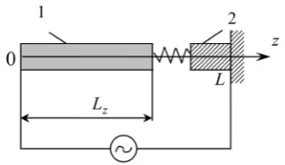
Parts of a rod shape are often used in engineering: dif-ferent shafts, axes of wheel sets, stocks, etc. The main type of defects for them is cross-cracks. A rod with a cross-crack is modeled by the system shown in Figure 1. The left part is considered to be elastically deformable, whereas the right part is a solid body and is fixed. We simulate a crack by a spring, where its equivalent stiff-ness is с. The total length of a rod is L. The unknown coordinate characterizing the location of a crack is Lz.
The natural oscillation in the system shown in Figure 1 can be initiated by a stroke impact from the left on the deformable part. In this case, the left part of the system moves as a solid, also deformations as longitudinal os-cillation arise in it.
Figure 1. The model of a rod with a crack.
of the rod:
( )
0
d d
0,
d d z
z
z L
z z L
U U
ES c U
z = z = =
= = −
. (1)
where U z t
( )
, is the displacement function, Е is the elastic modulus; S is the area of a cross section of a rod.We consider quasisolid motion of a rod (without any internal deformations). The differential equation looks like this if you do not consider the mechanical resistance:
0 0
mU = −cU . (2)
The quasisolid motion of a body occurs with a fre-quency:
0
c m
ω = . (3)
Since m=ρSLz, where ρ is the density of a rod
material. We obtain:
0 2
0 , or z
z
c c
L
SL S
ω
ρ ρ ω
= = . (4)
However, it is impossible to define Lz using just the
Equation (4), because the stiffness of the equivalent spring с is unknown. It depends on the size and shape of a crack, therefore cannot be assigned in advance.
Let us consider now elastic oscillation initiated in a rod taking into account the linear internal resistance, which is characterized by the coefficient β:
2 2
2 2 2
1
0
U U U
t
z β a t
∂ ∂ ∂
− − =
∂
∂ ∂ , (5)
where a2 E
ρ = .
We apply the Fourier method to the Equation (5):
( ) ( )
1n n
n
U q t Z z
∞
=
=
∑
. (6)Here qn
( )
t is generalized coordinates. Let us definethe eigen amplitude functions on the left end from the boundary condition (1):
( )
cos n ,(
1, 2, 3,)
n
p z
Z z n
a
= = , (7)
where pn is natural frequencies of elastic oscillation.
Taking into account the terms of orthogonality:
0
;
d 2
0;
z
L z
k n
L
k n Z Z z
k n
=
=
≠
∫
,we obtain the system of independent ordinary differential equations:
{
}
2
0, 1, 2, 3,
k k k k
q +βq +p q = k=
. (8)
Let us define the set of damped frequencies:
(
)
2
2 , 1, 2, 3,
4
k pk k
β
ω = − = . (9)
Using the boundary condition on the right end of the part 1, we obtain the equation of frequencies for damping oscillation:
ctg
n nLz ES
ac a
ω = ω
. (10)
Let us consider the Equations (4) and (10) together with n=1. If we eliminate the stiffness of an equivalent spring с, we obtain:
1 1
2 0
ctg z
z
a L
a L
ω ω
ω = . (11)
The values of frequencies ω0 and ω1 can be
fined experimentally. The concept of experimental de-fining of rod’s natural frequencies in case of longitudinal oscillation is described below. Using given values of ω0
and ω1, we can define Lz, which is the location of a
crack, by solving the Equation (11) numerically (or graphically).
In case of absence of a crack, quasisolid motion of any of its parts is excluded. Then, the first frequency of damping elastic oscillation can be defined by the well- known equation:
2 2
1
π
2 4
a L
β ω = −
. (12)
Thus, if the first frequency measured in an experiment coincides with the calculated value (12), we can conclude that the defect as a longitudinal crack is absent.
Note that the linear theory does not always take into account internal friction properly. Besides, the precise value of a coefficient β can be unknown for a given material. Therefore, we can calculate ω1 approximately
using the equation:
1 1
π 2
a p
L
ω ≈ = . (13)
3. Transformation of Longitudinal
Oscillation of a Rod into Electric Signals
defining natural frequencies of longitudinal oscillation of an elastic rod. We use the recently discovered potential component of the magnetic field [6-9]. It is described by the scalar functions H * or B*, that is why the term “scalar magnetic field” (SMF) is used. In contrast to a vector (vortex) component of a magnetic field, the scalar magnetic field is potential.
Conditions, under which a SMF can be created, and experiments with it are described in details in the mono-graph [6]. In particular, it is shown there that such a field can be created by a system of permanent magnets or a system of current circuits, for example a toroidal coil. The areas of a SMF are characterized by a sign: positive or negative. In a positive SMF, the longitudinal electro-magnetic force is directed along the current, in a negative SMF, it is against the current.
In the monograph [6], it was offered to rewrite the ge-neralized law of the electromagnetic force in differential form:
(
)
(
*)
*c Hc B
= ∇× × + ∇
f H B , (14)
where f is bulk density of magnetic force (Lorentz force); Hс is a vector of magnetic field strength of an intrinsic vortex magnetic field in a current-carrying con-ductor; B is magnetic flux density of an external vector magnetic field; B∗ is magnetic flux density of an ex-ternal SMF; Hс∗ is magnetic field strength of an intrin-sic SMF of a conductor.
It can be seen from the Equation (14) that transverse electromagnetic force is formed due to interaction of an intrinsic vector magnetic field of a conductor with an external vector magnetic field, whereas longitudinal force is formed due to interaction of an intrinsic scalar magnetic field of a conductor with an external SMF. Such an approach corresponds well to the common field theory and the Helmholtz’s theorem, because the super-position principle of solenoidal and potential components holds.
The certain similarity between phenomena of vortex and irrotational nature is observed. Along with the Am-pere’s force, which is perpendicular to the current, the magnetic force was discovered, which is directed along the current or against it depending on the sign of an ex-ternal SMF. The phenomenon of irrotational electro-magnetic induction [6], which is described by the law similar to the Faraday’s law, was discovered. It has been determined theoretically and experimentally that elec-tromotive force (EMF) of induction appears in a linear conductor while its translation in an external SMF. If we close the ends of a conductor, then the density current will be induced in an electrical circuit:
( )
( )
2
1
, d
z
z
U z t
j B z z
L t
σ ∗ ∂
=
∂
∫
, (15)where σ is conductivity of an electrical conductor. Re-sistance of a closed circuit is omitted.
This phenomenon can be used for experimental study-ing of the process of longitudinal oscillation in a resilient rod. Let us look at the task on longitudinal oscillation of an electrically conductive rod in a SMF. We assume that an external scalar magnetic field is created on some (ac-tive) section of a rod ∆ =z z2−z1 by induction
*
[image:3.595.317.486.427.507.2]B
(Figure 2). Let us consider the perfect case, when a SMF is fixed and homogeneous, and the boundaries of the active section are obviously determined. The ends of the rod are closed by an ideal electrical circuit with a fre-quency spectrum analyzer in it.
Let us write the differential equation for longitudinal oscillation of a resilient electrically conductive rod, based on the D’Alembert’s principle:
2 2
2 d 2 d d d 0.
c dH
U U U
S z ES z S z B S z
t dz
t z
ρ ∂ − ∂ +βρ ∂ − ∗ ∗ =
∂
∂ ∂
(16) The first term in the equation represents the fictitious force, the second term characterizes the elastic force, and the third one corresponds to the internal dissipation. The last term in the equation represents the electromagnetic force according to the law (14).
In the works [6-8], it is shown that the SMF Hc
∗
of a linear rod can be defined using the law similar to the Bi-ot-Savart-Laplace law:
1 1
. 4π
c
j H
z z z
∗= −
∆ − ′ ′
Consequently:
(
)
2 21 1
d d .
4π
c j
H z
z z z
∗= +
′ ′ ∆ −
The beginning of the crosshatched coordinate coin-cides with the left boundary of the active section. And
1
z′ = −z z Consequently, the equation for longitudinal magnetic force can be written like this:
(
)
*
2 2
1 1
d d
4π
j
F B S z
z z z
∗
= +
′ ′ ∆ −
.
Taking into account the Equation (15), we have:
(
)
( )
2 1 * * * 2 2 , 1 1d d d .
4π
z
z
U z t B
F S B z z
L z z z t
σ ∂
= + × ⋅ ′ ∂ ′ ∆ −
∫
(17)Note that this force has infinite values at the ends of the active section. This is because we used the model of a linear conductor, i.e. we omitted transverse sizes when calculating the SMF. Moreover, it was assumed that the SMF declines unevenly from some value to zero at the boundaries of the active section. Later, we will analyze a case close to real, when the SMF is heterogeneous and its strength equals zero at the ends of the active section. In this case, there is no uncertainty when calculating the longitudinal magnetic force.
Taking into account the Equation (17), the Equation (16) looks like this:
(
)
( )
2 2 1 2 2 2 2 * 2 2 , 1 1 d 0 4π z zU E U U
t
t z
U z t B
z
L z z z t
β ρ σ ρ ∂ ∂ ∂ − + ∂ ∂ ∂ ∂ − + = ′ ∂ ′ ∆ −
∫
(18)Let us apply the Fourier method using decomposition (6). We get:
(
)
2 2 1 2 2 1 * 2 2 d d 1 1 d 0 4πn n n n n
n
z
n n
z
E Z
Z q Z q q
z B
q Z z
L z z z
β ρ σ ρ ∞ = + − − + = ∆ − ′ ′
∑
∫
(19)Using amplitude functions (7) and the terms of ortho-gonality, we get the system of ordinary differential equa-tions:
(
)
{
}
2 2 2 1 1 2 2 2 2 2 1 π 2π 4 1 1 d d0, 1, 2, 3,
k k k
z z
z z
k n n
n
z z
Ek B
q q q
LL L
Z z q Z z
z z z k σ β ρ ρ ∗ ∞ = + + − + × ∆ − ′ ′ = =
∑
∫
∫
We introduce some notation:
(
)
2 2
1 1
2 2
1 1
d , d .
z z
k k n n
z z
Z z Z z
z z z
γ = + α =
∆ − ′ ′
∫
∫
We get:{
}
2 2 2 2 1 π 0 2π 41, 2, 3, .
k k k k n n
n z z
Ek B
q q q q
LL L
k
σ
β γ α
ρ ρ ∗ ∞ = + + − = =
∑
(20)Let us factorize the system (20) and rewrite it, so the first equation contains the first term of the sum, and the
second one has two terms, etc.:
(
)
2 2 2 2 2 2 21 1 1 1 2 1
2 2
2 2 2 2 2 2
2 1 1
2 2
3 3 3 3 2 3
3 1 1 2 2
1 π 0; 2π 4 2 π 2π 4 ; 2π 3 π 2π 4 ; 2π ; z z z z z z z z k B E
q q q
LL L
B E
q q q
LL L
B
q LL
B E
q q q
LL L B q q LL B q σ
β γ α
ρ ρ
σ
β γ α
ρ ρ
σ γ α
ρ σ
β γ α
ρ ρ
σ γ α α
ρ σ β ∗ ∗ ∗ ∗ ∗ ∗ + − ⋅ + ⋅ = + − ⋅ + ⋅ = + − ⋅ + ⋅ = + + −
(
)
2 2 2 2 21 1 2 2 1 1
π
2π 4
. 2π
k k k k
z z
k k k
z
k E
q q
LL L
B
q q q
LL
γ α
ρ ρ
σ γ α α α
ρ ∗ − − ⋅ + ⋅ = + + + (21) We can extract the equations for damped frequencies from here:
(
)
2 2 2 2 π, 1, 2, 3, 4 k k z k E h k L ω ρ
= − = . (22)
where
2
1
2 2π
k k k
z
B h
LL
σ
β γ α
ρ ∗ = − ⋅
is a damping factor of kth partial oscillation.
It can be seen that the process is polyharmonic, i.e.
there is oscillation of many frequencies. Every oscillation corresponds to a certain electrical signal appeared in a closed circuit. Using a frequency analyzer spectrum, we can extract and measure every frequency that is pre-sented in an experiment. Thus, we can use (11) to calcu-late the length Lz, which defines the location of a crack.
It can be seen from the Equations (20) and (21) that there is no electromagnetic effect on such oscillation at
0
k
γ = . Consequently, a corresponding electrical signal does not appear. It means that such oscillation will not be recognized by a frequency analyzer. In order to eliminate this case in an experiment, we need to change the loca-tion or the width of the active secloca-tion several times and measure accurately frequency, which is used (usually it is
1
ω ) by the spectrum analyzer.
homoge-neous SMF with sharply defined boundaries.
Let us analyze a case, which is more common, when the SMF is heterogeneous B∗ =B∗
( )
z . Generally, maximum one SMF is distinguished at a large gradient of its induction. Therefore, the boundaries of effective value*
B area can be defined quite accurately. Let us write the integral differential equation for natural longitudinal os-cillation in the resilient part of a linear rod in this case:
( )
(
)
( )
2 1 2 2 2 2 * * 2 2 1 1 d 0. 4π z zU E U U
t
t z
B z U
B z z
L z z z t
β ρ σ ρ ∂ ∂ ∂ − + ∂ ∂ ∂ ∂ − + = ′ ∂ ′ ∆ −
∫
(23)If we apply the Fourier method, we get:
( )
(
)
( )
2 1 2 2 1 * * 2 2 d d 1 1 d 0. 4πn n n n n
n
z
n n
z
E Z
Z q Z q q
z B z
q B z Z z
L z z z
β ρ σ ρ ∞ = + − − + = ′ ′ ∆ −
∑
∫
(24)We use eigen amplitude functions (7). We multiply the Equation (24) by Zk and integrate it from 0 to Lz. The
magnetic term is integrated from z1 to z2 like in the
pre-vious case. Applying the terms of orthogonality, we get the system of ordinary differential equations:
( )
(
)
( )
{
}
2 1 2 1 2 2 2 * 2 2 * 1 π 4 1 1 d 2πd 0, 1, 2, 3, .
k k k
z z k z z z n n n z Ek
q q q
L
Z B z z
LL z z z
q B z Z z k
β ρ σ ρ ∞ = + + − + ∆ − ′ ′ × = =
∫
∑ ∫
(25)Let us introduce some notation:
( )
(
)
(
)
2 1 * 2 2 1 1d , 1, 2, 3,
z
k k
z
Z B z z k
z z z η + = = ∆ − ′
∫
, (26)( )
(
)
2
1
*
d , 1, 2, 3,
z
n n
z
B z Z z=ψ n=
∫
. (27)Taking into account the notation introduced, the Equa-tions (25) will look like this:
{
}
2 2 2 1 π 0, 2π 41, 2, 3,
k k k k n n
n z z
Ek
q q q q
LL L
k
σ
β η ψ
ρ ρ ∞ = + + − ⋅ ⋅ = =
∑
(28)We factorize the system of Equations (28):
(
)
2 2 2
1 1 1 1 2 1
2 2 2
2 2 2 2 2 2
2 1 1
2 2 2
3 3 3 3 2 3
3 1 1 2 2
1 π
0,
2π 4
2 π 2π 4 , 2π 3 π 2π 4 , 2π 2π z z z z z z z z
k k k k
z
E
q q q
LL L
E
q q q
LL L
q LL
E
q q q
LL L q q LL k q q LL σ β ηψ ρ ρ σ
β η ψ
ρ ρ
σ η ψ
ρ σ
β η ψ
ρ ρ
σ η ψ ψ
ρ
σ
β η ψ
ρ + − ⋅ + = + − ⋅ + = ⋅ + − ⋅ + = ⋅ + + − ⋅ +
(
)
2 2 2 2
1 1 2 2 1 1
π 4 . 2π k z
k k k
z
E q L
q q q
LL
ρ
σ η ψ ψ ψ
ρ − −
= ⋅ + + + (29)
We write the equation for the set of natural damped frequencies:
(
)
2 2 2 2 π, 1, 2, 3, 4 k k z k E h k L ω ρ
= − = . (30)
where
1
2 2π
k k k
z
h
LL
σ
β η ψ
ρ
= − ⋅
is a damping factor of kth partial oscillation.
Let us analyze the particular case. Let the external SMF be distributed within the active section according to the following function:
( )
(
)
2* 2
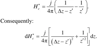
B z′ =λ ∆ −z z′ z′ . (31) Here λ is some dimensional constant, which defines maximum value of SMF induction. The diagram (31) is shown in Figure 3.
It can be seen on a diagram that the external SMF
( )
B∗ z′ equals zero at the ends of the active section, and is maximum in the center of the section. It corresponds well to SMF distribution, which can be created by a couple of flat magnets [6]. In case of such distribution of SMF, there is no uncertainty when calculating the longi-tudinal magnetic force.
We can see from the Equations (28) and (29), that at
( )
(
)
(
)
2 1 * 2 2 1 1d 0, 1, 2, 3,
z
k k
z
Z B z z k
z z z
η = + = =
∆ − ′ ′
∫
Figure 3. The distribution of a SMF in an active section.
tion, electrical signals, which correspond to some shapes of oscillation, are not present. In order to record effec-tively all natural frequencies, we need to change the lo-cation of the active section or its width several times.
The differential Equations (28) are more accurate comparing with (20), because they take into account the real distribution of a SMF.
4. The Concept of the Experiment
We describe the experimental installation and the me-thods of the experiment. The part analyzed has to be made out of electrically conductive material and have a shape similar to a rod. The geometry of a transverse sec-tion can be different if cross secsec-tion dimension is signif-icantly smaller than the length of the part. In addition, the cross sectional dimensions have to meet another re-quirement: an external SMF has to be as homogeneous as possible within the range of transverse coordinates.
The part is hung horizontally on elastic ropes. A ver-tical stop clamp fixes one of the part’s ends. It is neces-sary to eliminate electric contact between the part and the clamp. Conductors with small impedance are attached to the ends of the rod, which are enclosed in a frequency spectrum analyzer. The instrument used has to register small current impulses (µA) in a range of low frequen-cies (kHz).
The conditions of SMF initiation, its characteristics and topology are described in the monograph [6]. Small areas of the SMF are formed at the edges of a system of two flat magnets (Figure 4). We can define the sizes of the SMF area using for example images made out of iron filings (Figure 4(a)). The “empty” areas on the ends of the magnet couple is SMF. Magnetic field of such a sys-tem is equivalent to the magnetic field of a linear current with finite length: it has both vortex and potential com-ponent. The gradient of the SMF is directed along equiv-
(a) (b)
Figure 4. (а) The photograph of a field created by a couple
of flat magnets; (b) The distribution of the SMF created by a couple of flat magnets.
alent current (shown as the arrow (Figure 4(b))). That defines signs of the SMF areas.
In order to create a quite strong SMF, an inductor as a toroidal coil can be used. A vortex magnetic field in this case is concentrated inside of the coil, and a SMF of dif-ferent signs is formed on the edges of the toroid.
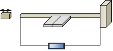
Cross sectional dimensions of the studying part cannot exceed sizes of the external SMF created by the inductor. The principal device of the experimental installation is shown in Figure 5.
A rod hanging horizontally sets against a heavy vertic-al wvertic-all. The end of the rod is fixed in a stop, so the rod cannot move away from the wall while testing. Conduc-tors with small resistance are attached to the ends of the conductors, and are connected to a frequency analyzer. In the left side of the figure, there is a striker. Its transverse section has to exceed cross sectional dimensions of a part tested. This provides plane shift of sections of the rod at elastic oscillation. An inductor of a SMF is situated so the rod’s transverse section is entirely inside of the SMF in some areas.
Let us describe the experiment technique (method) stage by stage.
Define the location and the width of an active section for an inductor of SMF that is used.
Create elastic oscillation by hitting horizontally the free end of the rod several times.
Measure first several frequencies starting with the frequency of quasisolid motion. It is necessary to change the location of the inductor several times in order to record oscillation of several first shapes without missing any.
Check if the first frequency coincides with the value calculated by the Equation (13). If yes, we conclude that there is no crack.
Calculate Lz using the Equation (11) in a case, when
the first experimental frequency differs significantly from one calculated by the Equation (13).
Let us give a numerical example. The following para-meters are given: the maximum value of induction of an external SMF is B∗
( )
z =1T;the conductivity of steel is6
7, 69 10 ;
m
σ = ⋅ Ω the density of steel is
3 kg
7800 ;
m ρ=
[image:6.595.310.538.86.155.2]Figure 5. The scheme of an experimental installation.
length of the rod studied is L=0.15m.
We calculate the first frequency of oscillation of the defect free rod using the Equation (13):
1
π 54308.867Hz 54.3kHz
2
a p
L
= = = .
We assume that the following frequencies were de-fined during the experiment:
1 1
0 tg 0.46kHz
z
z
a L
L a
ω ω
ω = ⋅ =
and ω =1 60kHz.
We solve the Equation (13) numerically and get:
0.1357m
z
L = .
5. Conclusion
Physical phenomena connected with a potential compo-nent of a magnetic field are discovered quite recently. The knowledge on new electromagnetic phenomena al-lows us to find innovative technical and technological solutions of applied problems.
The method of non-destructive testing, which we of-fered, uses the phenomenon of non-vortex electromag-netic induction. That makes it fundamentally new and differs from other known methods. It allows carrying out
non-destructive testing of a rod using a quite simple ex-perimental device, and defining the location of a crack.
The work is carried out within the frameworks of the RFFR grant No. 13-01-90904.
REFERENCES
[1] V. V. M. Kluev, “The Instruments for Non-Destructive Testing of Materials and Products,” Handbook on Me-chanical Engineering, 1985, 326 p.
[2] H. L. Libby, “Introduction to Electromagnetic Nonde-structive Test Methods,” Wiley-Interscience, New York, 1971.
[3] A. E. Levchin, “The Shock Pulse Method,” 2013. http://www.vibration.ru/spm/spm.shtml
[4] Y. V. Vankov, R. B. Kazakov and E. R. Yakovleva, “Natural Frequencies of a Product as an Informative In-dex of Defects,” Technical Acoustics, 2003.
http://cyberleninka.ru/article/n/sobstvennye-chastoty-izde liya-kak-informativnyy-priznak-nalichiya-defektov (The date of request: 01.10.2013).
[5] A. Akhtyamov and A. Karimov, “Diagnostics of crack location in a rod using natural frequency of longitudinal vibration,” Electronic Journal Technical Acoustics, No. 3, 2010, 6 p. http://www.ejta.org/en/karimov1
[6] A. K. Tomilin, “The Basics of Generalized Electro- dynamics,” 2009.
http://www.spbstu.ru/publications/m_v/N_017/frame_17. html
[7] A. K. Tomilin, “The Fundamentals of Generalized Elec-trodynamics,” 2008.
http://arxiv.org/ftp/arxiv/papers/0807/0807.2172.pdf [8] A. K. Tomilin, “The Potential-Vortex Theory of the
Electromagnetic Field,” 2010.
http://arxiv.org/ftp/arxiv/papers/1008/1008.3994.pdf [9] A. K. Tomilin, “The Potential-Vortex Theory of