Range finding of Alfvén oscillations and direction finding of ion cyclotron waves by using the ground based ULF finder

Range ®nding of AlfveÂn oscillations and direction ®nding

of ion-cyclotron waves by using the ground-based ULF ®nder

A. Guglielmi1_{, J. Kangas}2_{, D. Milling}3_{, D. Orr}3_{, O. Pokhotelov}1 1_{Institute of Physics of the Earth, 123810, Moscow, Russia}

2_{Department of Physical Sciences, University of Oulu, Linnanmaa, PO Box 333, FIN-90571 Oulu, Finland} 3_{University of York, Heslington, UK}

Received: 13 May 1996 / Revised: 14 November 1996 / Accepted: 10 December 1996

Abstract. A new approach to the problem of direction and distance ®nding of magnetospheric ULF oscilla-tions is described. It is based on additional information about the structure of geoelectromagnetic ®eld at the Earth's surface which is contained in the known relations of the theory of magnetovariation and magnetotelluric sounding. This allows us to widen the range of diagnostic tools by using observations of AlfveÂn oscillations in the Pc 3±5 frequency band and the ion-cyclotron waves in the Pc 1 frequency band. Preliminary results of the remote sensing of the magnetosphere at low-latitudes using the MHD ranger technique are presented. The prospects for remote sensing of the plasmapause position are discussed.

1 Introduction

The study is devoted to the problem of direction and range ®nding of the ULF geoelectromagnetic oscilla-tions. Our approach to this problem is in¯uenced by the paper of Hayakawa (1991) dedicated to the direction ®nding of VLF/ELF emissions (see also Hayakawaet al., 1991). We describe the operation of the ULF ®nder as a device which makes it possible to complete the range ®nding of Pc 3±5 oscillations (2±100 mHz) and the direction ®nding of Pc 1 waves (0.2±5 Hz). The range ®nder consists of a magnetometer and the recording system for measuring the Earth's currents, i.e. the normal set of standard observatory equipment. More-over, we consider a large volume of the Earth's crust in the vicinity of the observation point as an essential element of the device. The dimensions of the volume are assumed to be of the order of the skin depth. The electrodynamic characteristics of the new element are

taken into account when measurements and calculations are being carried out.

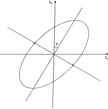
Figure 1 depicts a small part of the Earth's surface in the neighborhood of the observatory. Here thexaxis is directed northward, the y axis points eastward and the horizontal line stands for the projection of a magnetic shell on the Earth's surface. We consider that this shell undergoes resonant AlfveÂn oscillations and our purpose is to locate this shell. We present our method which allows us to solve this problem by observations at one single point. In other words, we suggest an algorithm for measurements and calculations to determine the dis-tancexRup to the projection of the oscillating magnetic

shell on the ground.

The ULF ®nder is also available for the Pc 1 wave propagation, i.e., for the measurement of the angle u (see Fig. 1). We start with this problem as it is easier in some respects than the range ®nding of Pc 3±5 oscillations. Although we cannot show any relevant Pc 1 data to verify the method at the moment, we introduce the basic elements of the direction ®nding method for the sake of completeness.

2 Direction ®nding of Pc 1 pulsations

a dense network of magnetometers (Hayashiet al., 1982, 1988). In addition to these methods we present here an independent technique for the measurement of azimuth u of the Pc 1 propagation (see Fig. 1). The position of the Pc 1 source region may be established by the direction ®nding of Pc 1 at two or more points.

Let us locate the observation point in the center of a region with a relatively homogeneous distribution of conductivity of the rocks in horizontal directions. We shall register three components of the magnetic ®eldb…t†

in the Pc 1 frequency band. The data analysis is based on the following graphic construction.

We can determine the plane perpendicular to b…t†. This plane intersects the horizontal plane (or Earth) in a straight line. The line rotates because the Pc 1 exhibits elliptic or, more precisely, quasi-elliptic polarization. The rotating line is coincident with the direction of Pc 1 propagation twice over the period of oscillations, much as a stopped clock shows the right time twice a day. This leads to the question: when does this coincidence take place? The answer runs as follows: the rotating line coincides with the propagation direction whenbz…t† ˆ0. Let us put this in another way. Figure 2 shows the hodograph of the vector-function bs…t†, where index s indicates that we are dealing with the horizontal vector projection. The moments at which bz…t† ˆ0 are indi-cated by the bold dots on the hodograph. Let us draw a line which connects these two points. Then the perpendicular to this line de®nes the direction of Pc 1 propagation.

In order to prove this conclusion we make use of the relation

bzˆik1rsbs; …1†

where 1stands for the surface impedance of the Earth, kˆc=x; cis the velocity of light,xis the frequency of

oscillations andbsˆ …bx;by†. This relation is widely used

in the study of the Earth's crust and upper mantle by means of magnetovariation sounding (Berdichevsky et al., 1969; Schmueker, 1970; Lilley and Sloane, 1976; Jones, 1980; PajunpaÈaÈ, 1988).

Setting bz ˆ0, we obtain rsbsˆ0. The operator rs may be replaced with iks, where ksˆ …kx;ky† is the

local wave vector of horizontal propagation. Hence

bsksˆ0, i.e., vector bs is parallel with respect to the

wave front, and it is perpendicular to the direction of propagation when bz ˆ0.

The information on the surface impedance is not necessary when the assumption of horizontal homo-geneity and isotropy of the Earth's crust in the vicinity of observation point is ful®lled. If it is necessary, we can take into account a weak dependence of 1on x;y. All one has to do is to replace bz by bzÿikbs r1. This

replacement follows from the evident generalization of Eq. (1) to the case of slightly inhomogeneous media:

bzˆikrs…1bs†. The realization of this version requires

preliminary investigation of the geoelectric structure of the region in the vicinity of the observation point to calculaterf. In this case the information on geoelectric properties of the rocks is used here in the explicit form.

Assuming the medium to be horizontally homoge-neous, but anisotropic we can use the procedure described, replacingbsby the auxiliary vector

biˆbj1kk1ÿji1 ;

where 1ij stands for the surface impedance tensor and

the indices i;j;k take the values x;y. Here we consider that 1ijˆ1ji.

Fig. 1.The location of the ULF ®nder (point at the origin of the coordinates) relative to the projection of the oscillating magnetic shell onto the ground (horizontal line). The inclined line indicates the direction of wave propagation in the ionospheric wave guide

Fig. 2.The hodograph of vector-functionbtˆs…t†: Thetwo pointsin

3 MHD ranger

We measure the east-west component of the electric ®eld

Ey and the vertical component of the magnetic ®eldbzin

the Pc 3±5 frequency range. Let us make use of spectral analysis and designate EˆjEy…x† j; Z ˆjbz…x† j. We

may ®nd the distance from the observation point to the magnetic shell, resonating at the frequencyx, from the expression

xR…x† ˆk…E=Z†sinh; …2†

if the electroconductivity of rocks has horizontal homogeneous distribution (Guglielmi, 1989). Here h…x† is the phase di€erence between the spectral componentsEy…x†andbz…x†. In the case of

inhomoge-neous distribution it is necessary to replace bz by

bzÿikbs r1as before.

Equation (2) was derived with the help of Eq. (1) and the impedance boundary condition

Esˆ1bsn; …3†

where ndenotes the unit vector normal to the Earth's surface directed earthwards (e.g., Wait, 1982), with regard to the approximate expression

bx…x† ˆbx…xR†‰1ÿi…xÿxR†Dÿ1Šÿ1 …4†

for the known spatial structure of the ®eld-line resonance (e.g., Hasegawa and Chen, 1974; Southwood, 1974; Orr and Hanson, 1981; Gough and Orr, 1984). HereDis the width of a resonance.

Let us draw an analogy between the range ®nding of ®eld-line resonances based on Eq. (3) and magnetotel-luric sounding (MTS). It is well known that the essence of MTS lies in the estimation of the vertical distribution of the crustal conductivity by the frequency dependence of the modulus of surface impedance (e.g., Rokityansky, 1982; Wait, 1982). The modulus of the surface im-pedance can be calculated from the Cagniard relation:

j1jˆE=H : …5†

HereHˆ jbxj, see Eq. (3). Clearly MTS is based on the

idea of compensation: since Ey and bx are proportional

to the intensity of external sources, their ratio …Ey=bx†

does not depend on this intensity and moreover it is proportional tof. (We recall thatEyis proportional tof,

and bx mostly does not depend onf.) In other words,

MTS is related to the compensation of the inde®nite conditions in the upper half-space. Similar to MTS, range ®nding in the form of Eq. (2) is achieved owing to a speci®c compensation: as both componentsEy andbz

are proportional to f, their ratio …Ey=bz† does not

depend onf. In other words, our method is directed to the compensation of inde®nite conditions in the lower half-space.

4 Veri®cation

As a test of the techniques described the data generously supplied by Prof. D. Chetaev has been analyzed in order to calculate xR. Pc 3 pulsations have been observed in

Ukraine not far from the village of Rakhny Sobovy,

/0ˆ43:9. Altogether 21 events suitable for analysis

were registered on August 30, 1974 between 09.30±12.30 LT. Each event represents a wave packet with a carrier frequencyf ˆx=2pand a smoothly varying amplitude envelope. In addition to the distance xR also the

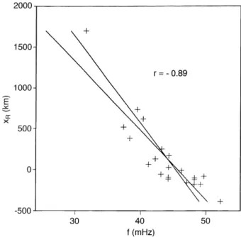
impedance jfjhas been calculated for selected events. The dependence ofxRonf is shown in Fig. 3. We can

see that the connection betweenxRandf is obvious. The

correlation coecient rˆ ÿ0:89 has the expected sign (the period T ˆ1=f increases with increasing latitude). The regression equation is

xRˆ3:76103ÿ82:7f ; …6†

where xRis measured in km andf in mHz, respectively.

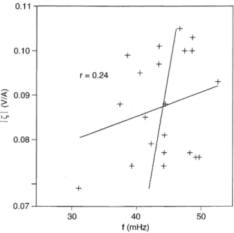
At the same time the connection betweenjfj andf

turned out to be rather weak (see Fig. 4). The correlation coecient rˆ0:24. This indicates that, at least in the case under study, the method of the magnetospheric MHD-range ®nding is more informa-tive than that of magnetotelluric sounding.

The result obtained may be veri®ed, for instance, by an observation in two points displaced in latitude. As such data is not available, we carried out indirect veri®cation by means of analysis of pulsation polariza-tion in the horizontal plane. Figure 5 displays the relative distributions of number of cases versus xRforL

and R polarizations separately. One can see that L

polarization is preferable if xR>0 and vice versa as

would be expected, in the framework of the theory of ®eld-line resonances (e.g., Lanzerotti, 1976).

With a knowledge of xR and the position of the

device, it is possible to determine the magnetic shell L

magnetosphere (e.g., Aubry, 1970; Jacobs, 1970; Orr, 1973; Orr and Matthew, 1971; Nishida, 1978). Accord-ing to Eq. (6)d lgq=dL' ÿ0:9 atL'2, which is not in contradiction with direct and indirect measurements (e.g., Carpenter and Anderson, 1992).

5 Discussion

We now discuss mainly two questions, one related to MTS and the other concerns HMD, and in one way or another both of these questions are related to the

problem of ULF ®nding. We point out also some limitations in using the direction ®nding method.

In order to understand the reason why the impedance 1is almost independent of the frequencyf (Fig. 4), let us consider the relation

Ey ˆ ÿ1 bx‡id 2

4 @

2_b x @x2

; …7†

which is more general than the Cagniard relation Eq. (5). Heredˆp2j1jkis the e€ective skin depth (e.g. Wait, 1982).

The strong inequality d2

4

@2_b x @x2

jbxj …8†

is usually valid, and that is why the second term on the right hand side of Eq. (7) may be omitted. Such a rejection leads to the violation of the correlation between 1 and f. Let us consider the question in a greater detail.

As we may write

@2_bx @x2 ˆ

2bx …D‡ixR†2 ;

it follows from Eqs. (1) and (4) that …D‡ixR† ˆ ÿk1bx=bzatxˆ0. Based on these relations we conclude

that the rejection of the second term in the right hand side of Eq. (7) leads to an error of the order of

…Z=H†2. The analysis of data indicates that the random variation of value…Z=H†2. The analysis of data indicates that the random variation of value…Z=H†2is of the order of 5±10%.

On the other hand, the relative variation of frequency is of the order of 10% (see Fig. 3). It is known that 1 depends on frequency such aspf in the high frequency limit, and 1 is almost independent on f in the low frequency limit. Hence, the regular variation of j1j in our case is not greater than 5%, i.e., it is less than a random variation. Therefore, the poor correlation betweenj1jandf is the result of neglecting the second term on the right hand side of Eq. (7).

A more detailed analysis of the data available for the present study reinforces our conclusion. It has been found that the correlation coecientrtends to increase with the increase of distance jxRj. For example,

rˆ0:41 ifjxRj>100 km (14 events), and rˆ0:07 if jxRj<200 km (14 events). The reason is that the greater jxRj, the smaller the second term in the right hand side

of Eq. (7).

We now turn our attention to the discussion of the application of ULF range ®nding to HMD. We see great possibilities for the development of hydromagnetic diagnostics with the help of the MHD-ranger. The idea is as follows. If the range-®nder is placed in the band of latitude 50ÿ60 _{it may be possible to detect the} plas-mapause positionLby recording Pc 3, 4 pulsations. It is anticipated that a display ofxRagainstf will reveal the

location of the plasmapause by a distinct discontinuity. There are two weak points which have to be recognized when applying the direction ®nding method Fig. 4.Magnetotelluric sounding at the same latitude on the same

date

developed in Sect. 2. Although Hayashi et al. (1982) found that the radius of the ionospheric secondary source of Pc 1 pulsations does not exceed 300 km it is obvious that the Pc 1 source region is often more extended in the E-W direction. On the other hand, according to the theoretical calculations (Grei®nger and Grei®nger, 1973; Fujita, 1987) the propagation of Pc 1 waves is limited mostly along the magnetic meridian plane i.e., at small values ofu. Although this may not be the general case according to our experience (see also e.g., Fraser, 1975) it is probable that the method to locate the Pc 1 source by the direction ®nding method does not work in all cases. However, it is expected that the method always produces useful information about the ¯uctuations of the local direction of the Pc 1 propagation.

Conclusion

The basic idea of the present study is that the impedance relationships between the components of electromag-netic ®eld on the Earth's surface can be used in hydromagnetic diagnostics. Two simple methods based on the impedance relation (1) have been introduced. This is not, however, an exact formula. We have avoided discussion of the applicability conditions but even so it is clear that the depth of ®eld penetration into the crust must be small as compared with the vacuum wavelength, the radius of curvature of the surface and the characteristic scales of the changes in the ®eld and medium properties along the surface of the Earth. Any complete answer to the question of applicability condition is dicult to present. The relationship (1) depends strongly on the geoelectric conditions in the vicinity of the point of observation. There is always the risk that one or another applicability condition will be violated or, alternatively, that some condition will turn out to be too rigid.

Is it possible to suggest an alternative approach which would retain the idea in general terms but which would not be based directly on Eq. (1)? We believe that the answer is positive. For this purpose we need to study the conductivity distribution in the lower half-space near the observation point by MTS methods and then jointly solve the internal problem (for the Earth's crust) and the external problem (for the magnetosphere). The solutions are to meet at the interface. Then, it becomes possible to use additional relationships between the ®eld compo-nents in order to improve the accuracy of magneto-spheric diagnostics.

Acknowledgments. This research was partly supported by the Commission of the European Union (Brussels) through Research Grant INTAS-94-2811. The authors are grateful to Professor Dmitrii Chetaev for the kind permission to use his data. We acknowledge also the stimulating comments and criticism of the referees.

Topical Editor K.-H. Glaûmeier thanks three referees for their help in evaluating this paper.

References

Aubry, M. P., Diagnostics of the magnetosphere from ground based measurements of electromagnetic waves, Ann. Geophy-sicae,26,341, 1970.

Berdichevsky, M. N., L. L. Vanyan, and E. B. Fainberg,Magnetic variation sounding using the space derivatives of ®eld, Geomagn. Aeronom.,9,229±301, 1969.

Carpenter, D. L., and R. R. Anderson,An ISEE/whistler model of equatorial density in the magnetosphere,J. Geophys. Res.,A97, 1097±1108, 1992.

Chetaev, D. N.,On the local structure of magnetotelluric ®eld,Izv. AN SSSR, Ser. Fiz. Zemli, 10,105±116, 1978.

Feygin, F. Z., Y. P. Kurchashov, V. A. Troitskaya, D. S. Fligel, and K. Dobes,Method of locating the Pc 1 source and hot plasma parameters in the generation region,Planet. Space Sci.,27,151± 158, 1979.

Fraser, B. J., Ionospheric duct propagation and Pc 1 pulsation sources,J. Geophys. Res.,80,2790±2796, 1975.

Fraser, B. J., and S. S. Wawrzyniak,Source movements associated with IPDP pulsations, J. Atmos. Terr. Phys., 40, 1281±1288, 1978.

Fujita, S.,Duct propagation of a short-period hydromagnetic wave based on the international reference ionosphere model,Planet, Space Sci.,35,91±103, 1987.

Gough, H., and D. Orr, The e€ect of damping on geomagnetic pulsation amplitude and phase at ground observatories,Planet. Space Sci.,32,619±628, 1984.

Grei®nger, C., and P. S. Grei®nger, Theory of hydromagnetic propagation in the ionospheric wave guide, J. Geophys. Res., 73,7473±7490, 1968.

Grei®nger, C., and P. Grei®nger, Wave guide propagation of micropulsations out of the plane of the geomagnetic meridian, J. Geophys. Res.,78,4611±4618, 1973.

Guglielmi, A.,Diagnostics of the plasma in the magnetosphere by means of measurement of the spectrum of AlfveÂn oscillations, Planet, Space Sci.,37,1011±1012, 1989.

Hasegawa, A., and L. Chen,Theory of magnetic pulsations,Space Sci. Rev.,16,347±359, 1974.

Hayakawa M., Direction ®nding of magnetospheric VLF/ELF emissions and their generation mechanism inEnvironmental and Space Electromagnetics, Ed. H. Kikuchi, Springer, Tokyo Berlin Heidelberg, 155±167, 1991.

Hayakawa M., K. Ohta, and S. Shimakura, Direction ®nding of very-low-latitude whistlers and their propagation in Environ-mental and Space Electromagnetics, Ed. H. Kikuchi, Springer, Tokyo Berlin Heidelberg, 168±171, 1991.

Hayashi, K., S. Kokubun, T. Oguti, K. Truruda, S. Mashida, T. Kitamura, O. Saka, and T. Watanabe, The extent of Pc 1 source region in high latitudes, Can. J. Phys.,59, 1097±1105, 1982.

Hayashi, K., T. Yamamoto, S. Kukubun, T. Oguti, T. Ogawa, N. Iwagami, T. Araki, T.-I. Kitamura, O. Saka, K. Makita, N. Sato, T. Watanabe, R. E. Horita, D. J. McEwen, J. S. Kim, and A. Egeland,Multi-station observation of Ipdp micropulsa-tions-two-dimensional distribution and evolution of the source region,J. Geomag. Geoelectr.,40,583±619, 1988.

Jacobs, J. A., Geomagnetic micropulsations, Springer, New York Berlin Heidelberg, 1970.

Jones, A. G., Geomagnetic induction studies in Scandinavia, J. Geophys.,48,181±194, 1980.

Lanzerotti, L. J.,Hydromagnetic waves: International symposium on solar-terrestrial physics, Boulder, Colorado, June 7±18, 1976. Lilley, F. E. M., and M. N. Sloance, On estimation electrical conductivity using gradient data from magnetometer arrays, J. Geomagn. Geoelectr.,28,321±328, 1976.

Manchester, R. N.,Correlation of Pc 1 micropulsations at spaced stations,J. Geophys. Res., 73,3549±3556, 1968.

Nishida, A.,Geomagnetic diagnosis of the magnetosphere, Springer, New York Berlin Heidelberg, 1978.

Orr, D.,Magnetic pulsations within the magnetosphere: a review, J. Atmos. Terr. Phys.,35,1±50, 1973.

Orr, D., and J. A. D. Matthew, The variation of geomagnetic micropulsation period with latitude and plasmapause, Planet. Space Sci.,19,897±905, 1971.

Orr, D., and H. W. Hanson,Geomagnetic pulsation phase patterns over an extended latitude array, J. Atmos. Terr. Phys.,43,894± 910, 1981.

PajunpaÈaÈ, K., Application of the horizontal spatial gradient technique to magnetometer array data in Finland,Rep. Dept. Geophys. Univ. Oulu, Oulu, Finland,15,1±14, 1988.

Rokityansky, I. I.,Geoelectric investigation of the Earth's crust and mantle, Springer, Berlin Heidelberg New York, 1982.

Schmueker, U., An introduction to induction anomalies, J. Geomagn. Geoelectr.,22,9, 1970.

Southwood, D. J.,Recent studies in micropulsation theory,Space Sci. Rev.,16,413±425, 1974.

Tepley, L., and R. K. Landsho€,Wave guide theory for ionospheric propagation of hydromagnetic emissions,J. Geophys. Res.,71, 1499±1503, 1966.