A Monte Carlo Algorithm for State and Parameter Estimation of Extended Targets

A Monte Carlo Algorithm for State

and Parameter Estimation of Extended Targets

Donka Angelova1and Lyudmila Mihaylova2

1

Institute for Parallel Processing, Bulgarian Academy of Sciences 25A Acad. G. Bonchev St, 1113 Sofia, Bulgaria

[email protected]

2

Department of Communication Systems, Lancaster University, South Drive, Lancaster LA1 4WA, UK

[email protected]

Abstract. This paper considers the joint state and parameter estimation of

ex-tended targets. Both the target kinematic states, position and speed, are estimated with the target extent parameters. The developed algorithm is applied to a ship, whose shape is modelled by an ellipse. A Bayesian sampling algorithm with finite mixtures is proposed for the evaluation of the extent parameters whereas a subop-timal Bayesian interacting multiple model (IMM) filter estimates the kinematic parameters of the maneuvering ship. The algorithm performance is evaluated by Monte Carlo comparison with a particle filtering approach.

1

Introduction

The increasing interest in simulation-based Bayesian methods for analysis of dynamic models has been resulted in a variety of powerful techniques for filtering and prediction of complex dynamic systems [1, 2]. The problem of state and parameter estimation of dynamic systems has many applications such as in signal processing, machine learning, robotics, target (e.g., aircraft, ship) tracking [3, 4]. In the present work, a Monte Carlo (MC) algorithm is applied to ship size evaluation in the framework of state filtering (tracking) of a maneuvering ship, modeled by a Markovian jump system.

Most of the target tracking algorithms available in the literature consider the moving object as a single point and estimate its state vector based on the incoming sensor data, e.g. range and bearing. However, recent sensor systems are able to resolve individual features or measurement sources on an extended object. The possibility to additionally make use of this measurements is referred to extended target tracking. For example, a high-resolution radar can provide a measure of down-range object extent given a rea-sonable signal-to-noise ratio [5, 6]. This valuable information can help for more precise estimation of the object behaviour. It can assist in resolving measurement association uncertainty in situations of closely spaced objects in dense clutter. Furthermore, the knowledge of objects size is especially important for the purposes of classification.

In this paper we address the problem of extended target tracking. There exist sev-eral ways for modelling object extent parameters. Models, based on measurements of

?

individual points on object require complicated techniques for multiple hypotheses test-ing [7]. A simple ellipsoidal object model is proposed in [5] and adopted in our work. The lengths of the major and minor axes of the ellipse have to be calculated, based on the measurements of down-range extent. Shape parameters are included in [5] in the state vector together with kinematic parameters and are estimated by Extended and Un-scented Kalman Filters (EKFs and UKFs) and particle filtering. However, it is pointed out is [5] that the EKF implementation is prone to divergence due to high nonlinearity conditions and a straightforward particle filter can avoid this problem.

Having in mind the inferences in [5, 6], we develop a Bayesian algorithm able to deal with the nonlinear estimation problem. Taking into account the possibility for sub-sequent classification, we assume that the unknown shape parameters are defined over the discrete set of values, with a given prior distribution. Within this formulation of the problem, data augmentation (DA) algorithm for finite mixture estimation [9] offers an alternative solution. DA represents a special case of Gibbs sampling [2] and belongs to the class of Markov Chain Monte Carlo (MCMC) methods. We develop a DA pro-cedure for the parameter estimation, along with an IMM algorithm for kinematic state estimation. The scheme implemented here is inspired by the ideas in [8].

The paper is organised as follows. Section 2 describes the system dynamics and measurement model. Section 3 presents the formulation of the problem. The designed DA algorithm is presented in Section 4. Section 5 illustrates and compares the perfor-mance of the proposed algorithm with a particle filter (PF). Conclusions are given in Section 6.

2

System Dynamics and Measurement Models

Target motion tracking is performed by a recursive reconstruction of the state proba-bility density function given the available prior information and current measurement data. Prior information includes dynamic models, models of the measurement process, initial state and noise probability distributions.

System Model. Consider the following model of a discrete-time jump Markov

sys-tem, describing object dynamics and sensor measurements

xk=f(mk,xk−1,θ) +g(mk,θ)wk, (1)

zk=h(mk,xk,θ) +d(mk,θ)vk, k= 1,2, . . . , (2)

where xk ∈ Rnx is the base (continuous) state vector, with transition function f, zk ∈ Rnz is the measurement vector with measurement function h, andθ ∈ Θ is a vector, containing unknown static parameters. The noiseswkandvkare independent

identically distributed (i.i.d.) Gaussian processes having characteristicswk ∼N(0,Q) andvk ∼ N(0,R), respectively. All vectors and matrices are assumed of appropri-ate dimensions. The modal (discrete) stappropri-atemk ∈ S , {1, 2, . . . , s} is a first-order Markov chain with transition probabilitiespij ,P r{mk =j|mk−1=i},(i, j∈S) and initial probability distributionP0(i),P r{m0=i},i ∈S, such thatP0(i)≥0, andPs_i=1P0(i) = 1.k= 1,2, . . .is a discrete time.

velocity in the Cartesian plane, centered at the observer location. All possiblesmotion regimes of the maneuvering ship are modelled by the modal state variablem. The static parameter vectorθ= (`, γ)0contains shape parameters: the length of the major axis of the ship ellipse`and the ratio of the lengths of the minor and major axesγ.

Measurement Equation. Similarly to [5, 6], we assume, that a high-resolution

radar provides measurements of rangerand bearingβ to the object centroid, as well as the object down-range extentLalong the observer-object line-of-sight (LOS). The relationship betweenLand the angleφbetween the major axis of the ellipse and the target-observer LOS is given by

L(φ) =`

q

cos2_φ+γ2_sin2_{(φ). (3)}

The measurement functionhin (2) is nonlinear,

h(xk,θ) = 

 p

(xk−xo)2+ (yk−yo)2

arctan((yk−yo)/(xk−xo))

L(φ(xk))



 (4)

where the measurement vector iszk = (rk, βk, Lk)0. Here(xo, yo)is the location of the observer. If it is assumed that the target ellipse is oriented so that its major axis is parallel to the velocity vector( ˙x,y˙)then from (3) the along-range target extent can be written in terms of the state vector andθas

L(φ(xk)) =θ(1)

q

cos2_{φ(xk) +θ(2)}2_sin2_φ(x

k), (5)

where φ(xk) = arctan ((xky˙k−x˙kyk)/(xkx˙k+yky˙k)).

The problem that we consider has own particularities: the measurements ofLare not used for the base state vector estimation. The kinematic states are estimated throughr

andβ. The estimated kinematic states are, however, used for the estimation of`andγ. This is the motivation for applying separate estimators to the two estimation problems.

3

Problem Formulation

The goal is to estimate the state vectorxkand the extent parameter vectorθ, based on all available measurement informationZk={z1,z2, . . . ,zk}. If we can calculate the

posterior joint state-size probability density function (PDF)

p

³

xk,θ|Zk ´

=

Z

p

³

θ|xk,Zk ´

p

³ xk|Zk

´

dxk, (6)

then for any integrable function~(xk,θ)the required estimate is given by

E

n

~(xk,θ)|Zk o

=

Z Z

~(xk,θ)p ³

θ|xk,Zk ´

p

³ xk|Zk

´

dθdxk. (7)

If we denote thel-th mode history, realised by a Markovian jump system through time

kasml

mixture with an exponentially increasing number of terms [10]

p³xk|Zk

´

=

εk X

l=1

p³xk|mlk,Zk

´

P³ml

k|Zk ´

. (8)

The exponentially increasing computations can be avoided by different ways of com-bining histories of models. For example, the Interacting Multiple Model (IMM) filter

[10] provides an approximate state estimatexˆk =E n

~(xk)|Zk o

and its associated covariance matrixPk, by usingsworking in parallel EKFs. Then the estimate ofθcan

be expressed asθˆk=E n

~(θk)|xˆk,Zk o

. Note that thekindex ofθindicates that it is

calculated based on the information up to time instantk, not thatθis time-varying. MC algorithms (PF or MCMC) can be applied to the highly nonlinear extent estima-tion problem. The use PF for the first step is not justifiable, as ships exhibit moderate maneuvers and the time interval between the measurements is rather short. Since the size estimate could be obtained along with the filtering process, but not necessary on-line, the more precise MCMC algorithm can be applied.

The scheme implemented here is similar to [8]. It comprises the following steps. On receipt of a new measurementzk:

a) run the IMM algorithm with the previous state estimatexˆk−1in order to update the current state estimatexˆk.

b) find the estimateθˆk of the parameter vectorθbased on the previous estimates

ˆ

θk−1,xˆk, and the measurement likelihoodp ³

zk|θˆk−1,zk−1 ´

, by PF or DA scheme.

4

Extent Parameters Estimation by Stochastic Simulation

Based on a priori information about ship types, we assume thatθtakes values from a known discrete setθ ∈ T ,{1, 2, . . . , t} with known prior distribution:Pθ0(i) , P r{θ=i},i ∈T, such thatPθ0(i)≥0, and

Pt

i=1Pθ0(i) = 1. Let us suppose that

along-range extent measurementsLk, k= 1, . . . , n, . . .have Gaussian distributed zero-mean errors with known varianceRL. The PDF of the measurementLkis represented in the following mixture form [9, 11]:

p(Lk|π,θ,xk) =

t X

j=1

πjG(Lk|θj,xk), (9)

whereπ = (π1, . . . , πt)are the mixture proportions which are constrained to be non-negative and sum to unity.G(Lk|θj,xk)∼N(Lk;L(θj,xˆk), RL)is a Gaussian den-sity andL(θj,xˆk)is the measurement prediction, calculated according to (5). Thus, the task is reduced to the well known finite mixture estimation problem: for the mix-ture model (9) with known component PDFs G(Lk|θj,xk), one needs to estimate the unknown weights π = (π1, . . . , πt), given a sequence of independent observa-tions L1, L2, . . . , Ln. The mixture component with a maximum weight identifies the

most probable ship type. The estimate of the extent parameters can be calculated as the

Mixture Weights Estimation by Data Augmentation. DA algorithm approximately

evaluates the mixture posterior distribution, relying on the missing data structure of mixture model. Generally, the mixture model is given by the observation ofn indepen-dent random variablesy1, . . . , ynfrom at-component mixture [9, 11],

z(yk) = t X

j=1

πjzj(yk), k= 1, . . . , n, (10)

where the densitieszj, j= 1, . . . , tare known or are known up to a parameter and the proportionsπjsatisfy the above conditions. We consider the special case, where only the weightsπhave to be estimated. According to [9], the mixture model can always be expressed in terms of missing (or incomplete) data. That is, define vectorsδ(k) =

(δ1(k), δ2(k), . . . , δt(k)),k = 1, 2, . . . , nwith componentsδj(k) ∈ {0,1}, j =

1,2, . . . , t, which indicate that the measurementykhas densityzj(yk) [8]. The model

is hierarchical with, on top, the true parameters of the mixture,π, then the missing data whose distribution depends onπ,δ ∼ p(δ|π), and, at the bottom, the observed data y ∼p(y|π,δ). Starting with an initial valueπ(0), the algorithm implements two-step

iterative scheme: at the iterationu, u= 1,2, . . .

a) generateδ(u)∼p(δ|y,π(u))from a multinomial distribution with weights pro-portional to the observation likelihoods:δ(u)_j (k)∝π(u)_j zj(yk);

b) generateπ(u+1)∼p(π|y,δ(u)).

Since the conjugate priors onπ are with Dirichlet distributions (DD)D(α1, . . . , αt) [9],π(u+1)_{is generated according to the DDs with parameters, depending on the} miss-ing data. Bayesian samplmiss-ing produces an ergodic Markov chain (π(u)_{) with} station-ary distributionp(π|y). Thus, afteru0initial (warming up) steps, a set ofU samples

π(u0+1)_{, . . . , π}(u0+U)_{are approximately distributed asp(π|y)and, due to ergodicity,}

averaging can be made with respect to time [8, 9].

In the next scheme, the sequence of observationsyk, k = 1, . . .is replaced by the along-range extent measurementsLk, k= 1, . . .. The joint IMM and data augmentation scheme is given below. DA is realised in a sliding window mode.

Algorithm Outline

Fork= 1,2, . . .

• Run the IMM algorithm with the previous state vectorxˆk−1, covariance ma-trixPk−1and posterior model probability vectorµk−1 to update the current estimatexˆk, together withPkandµk.

• Compute Mixture Components Conditional PDFs

˜

Gj(k),G(Lk|θj,xk)∝exp

h

−0.5 (Lk−L(θj,xˆk))TR−1L (Lk−L(θj,xˆk)) i

• Implement Data Augmentation - Initialisation: π(0) _=π(k−1) - Iterations (u= 0,1, . . . , u0+U−1)

* Missing Data Conditional Probability Mass Functions (PMFs)

q(u)_j (l) = π

(u) j G˜j(l) P_t

j=1π (u) j G˜j(l)

* Missing Data Generation (Multinomial Sampling)

δ(u)_{(l) = (0, . . . ,0, 1,0, . . . ,0)∼}n_q(u) j (l)

ot

j=1, l= 1,2, . . . k

* Parameter Evaluation (Dirichlet Distribution Sampling)

π(u+1)_{∼ D} Ã

π;α1+ k X

l=1

δ(u)₁ (l), . . . , αt+

k X

l=1

δ(u)t (l)

!

• Calculate the Output Estimates

π(k) = 1

U

U X

σ=1

π(u0+σ) _{and θ}ˆ

k= t X

j=1

πj(k)θj

5

Simulation Results

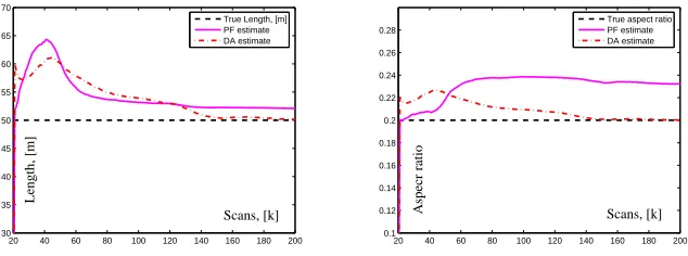
The algorithm performance is evaluated by simulations over trajectories, including con-secutive segments of uniform motion and maneuvers (a typical scenario is shown in Fig.1(a)). The observer is static, located at the origin ofx−y plane. The initial tar-get state isx0= (18e3,−14,90e3,5)0. It performs two turn maneuvers with a normal acceleration of ±1.4 [m/s2]. The object length is ` = 50 [m] and the ratio of the lengths of the minor and major axes (aspect ratio) isγ = 0.2. The sensor parame-ters are as follows [6]: sampling intervalT = 0.2 [s]; the standard deviations of mea-surement errors along range, azimuth and along-range target extent are respectively:

σr= 5 [m],σβ= 0.2degandσL= 5 [m].

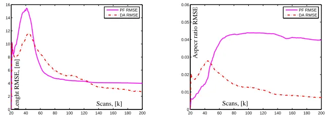
Root-Mean Squared Errors (RMSEs) [10] are selected as a quantitative measure for the

algorithm performance evaluation.

An IMM algorithm with s = 3 models is designed. The first model corresponds to the nearly constant velocity motion. The next two models are matched to the nearly coordinated turn maneuvers with a turn rate of ω = ±1.4 [rad/s]. The form of the transition matrices in (1) for these models can be found in [10].

A particle filter for extent parameters estimation is realised for the purposes of compar-ison with DA algorithm, withN = 100particles. Similarly to the procedure, described in [1] (Ch.10),N particles(θ(i))N

i=1 are generated according to a priori normal dis-tribution with mean, corresponding to the trueθ. After that the particles are predicted according to a normal distribution with small deviations to provide “artificial evolution” of parameters. Then the particle weights are evaluated using likelihoods of the received measurements and finally resampling is implemented according to a known rule.

θwith a high probability. The results are obtained from one MC realisation and confirm the reliability of the algorithm for classification tasks.

Figs.(2) and (3) demonstrate the better performance of the DA in comparison with the PF: the estimation errors of`andγobtained by the PF are quite large. It is natural to ex-pect a better performance of DA scheme. It has additional prior information, available from the θ set. DA is an off-line procedure and processes the cumulative measure-ment information. In addition, PF involves additional noise, necessary for prediction which deteriorates the estimation accuracy of the parameters (they are fixed). Its perfor-mance is highly sensitive to the choice of noise deviations, which are design parameters. However, the better performance is achieved at the increased computational time. The relative execution time is approximately 17:1 in PF favour.

1.74 1.75 1.76 1.77 1.78 1.79 1.8

x 104

8.992 8.993 8.994 8.995 8.996 8.997 8.998 8.999 9 9.001

9.002x 10

4

x [m]

y [m] START

1 2 3 4

0 0.1 0.2 0.3 0.4 0.5 0.6 0.7 0.8

θ set

mixture weights,

π

Fig. 1. Object trajectory and Mixture proportionsπ

20 40 60 80 100 120 140 160 180 200

30 35 40 45 50 55 60 65 70

Scans, [k]

Length, [m]

True Length, [m] PF estimate DA estimate

20 40 60 80 100 120 140 160 180 200

0.1 0.12 0.14 0.16 0.18 0.2 0.22 0.24 0.26 0.28

Scans, [k]

Aspecr ratio

True aspect ratio PF estimate DA estimate

Fig. 2. PF and DA comparison: True and estimated`andγ

6

Conclusion

20 40 60 80 100 120 140 160 180 200 0

2 4 6 8 10 12 14 16

Scans, [k]

Lenght RMSE, [m]

PF RMSE DA RMSE

20 40 60 80 100 120 140 160 180 200

0 0.01 0.02 0.03 0.04 0.05 0.06

Scans, [k]

Aspecr ratio RMSE

PF RMSE DA RMSE

Fig. 3. PF and DA comparison: RMSE of`andγ

parameter estimation of a ship, based on positional and along-range object extent mea-surements. A Monte Carlo algorithm (Data augmentation) is designed for length and aspect ratio assessment of the elliptical ship shape. The performance of the proposed al-gorithm is evaluated by Monte Carlo simulation. The results show that DA is capable to deal with highly nonlinear relationships between states, parameters, measurements and complicated target-observer geometry. A combined IMM-DA procedure is proposed which provides accurate joint state-parameter estimation and reliable identification of the ship type.

References

1. Doucet, A., de Freitas, N., Gordon, N. (ed.): Sequential Monte Carlo Methods in Practice. Springer-Verlag, New York, (2001).

2. Liu, J.: Monte Carlo Strategies in Scientific Computing. Springer-Verlag, New York, (2003). 3. Storvik, G.: Particle filters in state space models with the presence of unknown static

para-meters. IEEE. Trans. of Signal Processing, Vol. 50, No. 2, (2002) 281–289.

4. Doucet, A., Tadic, V.: Parameter estimation in general state-space models using particle methods. Ann. Inst. Stat. Math., vol. 55, No. 2, (2003) 409–422.

5. Salmond, D., Parr, M.: Track maintenance using measurements of target extent. IEE Proc.-Radar Sonar Navig., Vol. 150, No. 6, (2003) 389–395.

6. Ristic, B., Salmond, D.: A study of a nonlinear filtering problem for tracking an extended target. Proc. Seventh Intl. Conf. on Information Fusion, (2004) 503–509.

7. Vermaak, J., N. Ikoma, S. Godsill: Sequential Monte Carlo Framework for Extended Object Tracking. IEE Proc.-Radar Sonar Navig., Vol. 152, No. 5 (2005), 353–363.

8. Jilkov, V., Li,X. Rong, Angelova, D.: Estimation of Markovian Jump Systems with Unknown Transition Probabilities through Bayesian Sampling. LNCS, Vol. 2542 (2003), Springer-Verlag, Berlin, pp. 307-315.

9. Diebolt, J., Robert, C.P.: Estimation of Finite Mixture Distributions through Bayesian Sam-pling. J. of Royal Statist. Soc. B 56, No. 4, (1994) 363–375.

10. Bar-Shalom, Y., Li, X.R., Kirubarajan, T.: Estimation with Applications to Tracking and Navigation: Theory, Algorithms, and Software. Wiley, New York (2001).