Borrowing Constraints, Multiple Equilibria and Monetary Policy

Munich Personal RePEc Archive

Borrowing Constraints, Multiple

Equilibria and Monetary Policy

Assenza, Tiziana

CeNDEF, University of Amsterdam

2007

Borrowing Constraints, Multiple Equilibria and

Monetary Policy

Tiziana Assenza

CeNDEF, University of Amsterdam

Abstract

The appealing feature of Kiyotaki and Moore’s Financial Accelera-tor model (Kiyotaki and Moore, 1997, 2002) is the linkage of asset price changes and borrowing constraints. This framework therefore is the nat-ural vehicle to explore the net worth channel of the monetary transmission mechanism. In the original model, however, all the variables, credit in-cluded, are in real terms. In order to assess the impact of monetary policy the model must be reformulated to …t a monetary economy. In the present paper we model a monetary economy with …nancing constraints adopt-ing the Money In the Utility function (MIU) approach.The occurrence of multiple equilibria is a likely outcome of the dynamics generated by the model. A change in the growth rate of money supply can a¤ect real out-put throughthe impact of in‡ation on net worth. In a sense the monetary transmission mechanism we are focusing on consists of a combination of thein‡ation tax e¤ect and thenet worth channel. Contrary to the tra-ditional view, at least for some parameter restrictions, an increase of the in‡ation tax can bring about an increase of aggregate output.

1

Introduction

The impact of monetary policy economic activity has been and still is a funda-mental question in macroeconomics. The literature has proposed several di¤er-ent mechanisms to explain the propagation of monetary shocks. During the ‘90s a remarkable body of literature has been developed under the name of…nancial acceleratorornet worth channelto explore the transmission of monetary policy on investment and production through the impact on …rms’ …nancial structure. The ambitious scope of this branch of literature consists in understanding the mechanism through which adverse shocks, in particular a contractionary mon-etary policy, a¤ect the decisions of …rms, households, …nancial intermediaries and investors and cause large and persistent e¤ects on economic activity and in‡ation.

In the early ’90s two alternative frameworks have been proposed to model the Financial Accelerator hypothesis. Bernanke-Gertler (1989, 1990) and co-authors emphasized the role of agency costs in the decision to supply credit while Greenwald-Stiglitz (1988, 1993) focused on the role of bankruptcy costs in limiting investment and production. In the late ’90s Kiyotaki and Moore (1997, 2002) put forward a new framework based on the idea that borrowers face a …nancing constraint because lenders extend credit up to the present value of borrowers’ collateralizable wealth, i. e. “land”, which proxies real assets. The novel and appealing feature of their model is the linkage of asset price changes and borrowing constraints: booming asset prices relax borrowing constraints and boost economic activity; the upswing, in turn, a¤ects asset prices.

Thanks to this feature this model is the natural vehicle to explore the balance-sheet channel of the monetary transmission mechanism.In the original model, however, all the variables, credit included, are in real terms. Therefore the model as such is not suitable to explore the e¤ects of monetary policy. In order to assess the impact of a such a policy, the model must be reformulated to …t a monetary economy with borrowing constraint. An attempt in this direction has been proposed by Cordoba and Ripoll (2004), who introduce a cash in ad-vance constraint for consumption and investment to analyze the role of collateral constraints as a trasmission mechanism of monetary shocks. The major result of their model is that a monetary shock can generate persistent movements in aggregate output. The amplitude of this movements depends on whether or not debt contracts are indexed.

In our paper we follow a well known but di¤erent route. We model a mon-etary economy with …nancing constraints adopting the Money In the Utility function (MIU) approach. 1

As in KM population consists of …nancially constrained farmers and non

1_{The introduction of money in the utility function is a controversial but well known and}

constrained gatherers. In the present framework, however, preferences are non linear: they are represented by a Cobb-Douglas utility function whose argu-ments are consumption and money holdings. As in in the original framework, there are two types of goods, a non storable consumption good (fruit) and a collateralizable, durable asset/input (land). The total supply of land is given and constant.

By assumption the farmer and the gatherer have access to di¤erent tech-nologies. The farmer is endowed with a linear technology while the gatherer has a well behaved production function. Notice however, that since preferences are non-linear in consumption, we must not assume that part of production is non-tradable and that consumption is limited to bruised fruit as in Kiyotaki and Moore.

In this setting, we study the e¤ects of a monetary injection on the asset price and the allocation of land to the farmers and the gatherers. By assumption, the farmer is less patient than the gatherer.2 _{Moreover, in equilibrium the real}

interest rate is anchored to the rate of time preference of the gatherer. Since the rate of time preference of the gatherer is exogenous, the real interest rate is given and constant. As a consequence, a change of the in‡ation rate brings about the same change in the nominal interest rate. Finally, in the steady state the in‡ation rate is pinned down to the rate of growth of money supply. In the end therefore, in the steady state a change of the rate of growth of money supply brings about a change of the same sign and the same magnitude of the nominal interest rate.

In the present context, therefore, by construction an expansionary monetary policy cannot a¤ect real output through theliquidity e¤ect. By construction in fact the liquidity e¤ect is not active because, in the end, an increase in the rate of growth of money supply raises the in‡ation rate and pushes the interest rate up, not down. This does not necessarily mean, however, that superneutrality always holds. A change in the growth rate of money supply can a¤ect real output throughthe impact of in‡ation on net worth. In a sense the monetary transmission mechanism we are focusing on consists in a combination of the

in‡ation tax e¤ect and the net worth channel. Contrary to the traditional view, at least for some parameter restrictions, an increase of the in‡ation tax can bring about an increase of aggregate output.

The paper is organized as follows. In sections 2 and 3 we discuss the opti-mization problems of the farmer and the gatherer respectively. In section 4 we present the equilibrium conditions and in section 5 we discuss the dynamics gen-erated by the model. In particular we explore the e¤ects of a monetary shock. In sections 6 and 7 we present the e¤ects on individual and aggregate variables of unexpected and temporary shocks to the productivity parameter and to the rate of growth of money supply respectively.

2_{Another way of characterizing the framework put forward by Kiyotaki and Moore, in fact,}

2

The farmer/borrower

Preferences of both the farmer and the gatherer are de…ned over consumption and real money balances. Adopting a Cobb-Douglas speci…cation of the utility function, preferences of the farmer are represented by:

UF =

1

X

s=0

F s _lncF

t+s+ (1 ) lnmFt+s (1)

where 0 < < 1; cF

t+s is consumption and mFt+s =

MF t+s

Pt+s

are real money balances. We assume that the production function of the farmer has constant returns to scale: yF

t = KtF1whereyFt is output of the farmer,KtF1is land he

owns int 1and >0.3

The farmer maximizes utility subject to two constraints: the ‡ow-of-funds (FF) constraint and the …nancing constraint. Following Ljungqvist and Sargent (2000) we assume thatat the beginning of period tthe farmer decides the amount of money he wants to holdat the beginning of periodt+1. Therefore the farmer’s ‡ow of funds constraint in nominal terms is:

PtytF+Bt+MtF Qt KtF KtF1 +NtBt 1+PtcFt +MtF+1

where PtyFt is nominal income, MtF are money balances at the beginning of

periodt, Bt is credit obtained in t, MtF+1 are money balances that the farmer

wants to hold at the beginning of period t+ 1, Qt is the price of land and

Nt= 1 +itis the gross nominal interest rate.

Dividing byPtwe obtain the FF constraint in real terms:

cF

t + (1 + t+1)mFt+1+qt KtF KtF1 KtF1+mFt +bt Rbt 1

where t+1:=

Pt+1

Pt

1is the in‡ation rate, qt:=

Qt

Pt

is the real price of land,

bt:=

Bt

Pt

is credit in real terms and R= 1 +r:= 1 +it 1 + t+1

is the real interest rate.

In order to establish the way in which liquidity changes over time, let’s as-sume that each agent gets a transfer in money in t+ 1from the public sector proportional to his money holdings int: Ti

t+1 = gMMti; i = F; G, where the

superscriptF (G) denotes the farmer (gatherer). The supply of money, there-fore, follows the law of motionMi

t+1 =Mti+Tti+1 = Mti(1 +gM). In words,

money holdings grow at the (exogenous) rategM. In order to keep the analysis

as simple as possible we assume that the rate of change of money supplygM is

uniform across agents. This means that the allocation of money to the agents, i.e. the ratio of money of the farmer to money of the gatherer, is constant

3_{Since preferences are not linear in consumption we must not distinguish between tradable}

(which will be denoted by in the following). Therefore real money balances of the agent int+ 1aremi

t+1:=

Mi t+1

Pt+1

= M

i t

Pt

1 +gM

1 + t+1

=mi t

1 +gM

1 + t+1

. Substituting this relation into the FF constraint we get:

cFt +gMmFt KtF1 Rbt 1 qt KtF KtF1 +bt (2)

The termgMmFt =

MF

t+1 MtF

Pt

is the increase in the farmer’s money hold-ings betweent and t+ 1in real terms, i.e. at prices of periodt. For lack of a better term we will refer to this magnitude as the increase in real money bal-ances. In the light of this remark, (2) can be interpreted as follows: “resources” of the farmer, of internal or external origin ( KF

t 1andbtrespectively), can be

employed to consume (cF

t), “invest” (qt KtF KtF1 ), reimburse debt (Rbt 1)

and increase money balances (gMmFt). The increase in desired money balances

is always equal to the increase of liquidity engineered by the central bank by means of money transfers. In other words, we are ruling out the mismatch between desired and actual increase in money holdings.

The farmer is also …nancially constrained, the …nancing constraint can be expressed as:

bt

qt+1

R K

F

t (3)

The farmer maximizes (1) subject to the FF constraint (2) and the …nancing constraint (3). From the Lagrangian:

L =

1

X

s=0

F s _lncF

t+s+ (1 ) lnmFt+s +

+

1

X

s=0

F s F

t+s KtF1+s Rbt 1+s+

qt+s KtF+s KtF1+s +bt+s gMmFt+s cFt+s +

+

1

X

s=0

F s t+s

qt+1+s

R K

F

t+s bFt+s

we obtain the followingFOCs: (iF) @L

@cF t

= 0 =)

cF t

= Ft

(iiF) @L @cF

t+1

= 0 =)

cF t+1

= Ft+1

(iiiF) @L @mF

t

= 0 =) 1

mF t

= FtgM

(ivF) @L @mF t+1

= 0 =) 1

mF t+1

= Ft+1gM

(vF) @L @bF t

(viF) @L @bF

t+1

= 0 =) F_{t+1 t+1} R F

t+2 F = 0

From (iF) and (iiF) follows that the FF constraint is binding in each period. From (iF)-(ivF) follows:

gMmFt =

1

cFt 8t (4)

i.e. the ratio of the increase in money holdings gMmFt to consumption cFt is

constant and equal to 1 . Notice that, given the rate of growth of money supplygM;the equality above states that the ratio of consumption to real money

balances is constant.

From (vF) and (viF) we conclude that the …nancing constraint is binding if:

F t F t+1

> FR (5)

Moreover after trivial substitutions we get:

F t F t+1

= c

F t+1

cF t

=m

F t+1

mF t

(6)

i.e. consumption and real money balances should grow at the same rate. This condition ensures that the ratio of consumption to real money balances remains constant as implicitly stated in (4).

From (5) and (6) follows: cF

t+1

cF t

= m

F t+1

mF t

> FR

Notice that m

F t+1

mF t

= 1 +gM 1 + t+1

by construction. Therefore from (6) we conclude

that consumption grows at the rate 1 +gM 1 + t+1

.

In the end, the …nancing constraint is binding if the following condition holds:

1 +gM

1 + t+1

> FR

In the steady state real money balances are constant, i.e. the rate of growth of money balances is equal to the in‡ation rategM = . The inequality above,

therefore, boils down to:

R < 1_F

The same condition holds also in the original KM framework. Since both the ‡ow of funds and the …nancing constraints are binding, we can write

cF

where t=qt

qt+1

R is the downpayment. In other words, the output produced by the farmer is employed to consume, hold money balances and provide the downpayment. Given output, the higher the rate of growth of nominal money balances, the smaller consumption and/or downpayment, the smaller therefore the investment in landholding.

Substituting theFOCs into the ‡ow of funds constraint we get the optimal level of consumption and real money balances:

cF

t = KtF1 tKtF (7)

gMmFt = (1 ) KtF1 tKtF (8)

Thanks to the Cobb-Douglas speci…cation of preferences, consumption and the increase in real money balances are a fraction and 1 respectively of the resources available to the farmer, which in turn are equal to output less down-payment.

Since both the FF and the …nancing constraints are binding, from the very de…nition of net worth in the present context, we can conclude that net worth is equal tosaving net of the increase in real money balances:

nF

t =yFt cFt gMmFt RbFt 1+qtKtF1=sFt gMmFt (9)

In KMnF

t =sFt. The increase in real money balances therefore is a negative

component of net worth. In the steady stategM = so that

nF =sF mF

An increase in the rate of growth of money (which translates into an increase of in‡ation) has anin‡ation tax e¤ect on the accumulation of net worth.

Making use of (4), after some algebra we can rewrite the equation above as:

nF

t = KtF1

1 cF

t = KtF1 gMmFt

where = 1

1 . In words: net worth is equal to output minusa multiple of the increase in real money balances. Other things being equal the higher the increase in real money balances, the lower net worth.

Finally notice that since the sum of consumption and the increase in real money balances is equal to the resources available to the farmer, net worth is devoted completely to downpayment:

nF

t =ytF cFt +gMmFt =ytF ytF tKtF = tKtF (10)

The same condition holds in KM. Considering (9) and (10) simultaneously we infer that in a KM economy with money

nF

In the steady state

sF = KF+ mF

Part of the resources of the farmer cannot be employed as downpayment because they must be devoted to pay the in‡ation tax.

After trivial substitutions from the ‡ow of funds constraint one gets:

KtF =

1

t

KtF1 gMmFt (11)

Equation (11) is the law of motion of the land of the farmer. Notice that it di¤ers from the law of motion obtained by KM due to the term that represents the increase of real money balances. In particular there exists a negative relation between the demand for land and the demand for money: the higher the real money balances demanded by the farmer the lower landholding and viceversa. In the steady state KF _{= K}F _{+ m}F_{. An important implication of this}

equation is that m

F

KF = : With the exception of a zero-in‡ation steady

state, therefore,

< (12)

:

3

The gatherer/lender

Following the same modelling strategy of the previous section, we assume that preferences of the gatherer are represented by a Cobb Douglas utility function:

UG =

1

X

s=0

G s _lncG

t+s+ (1 ) lnmGt+s (13)

where the meaning of the symbols is straightforward. Being unconstrained from the …nancial point of view, the gatherer maximizes utility subject only to the ‡ow of funds constraint.

We assume that the production function of the gatherer has decreasing re-turns to scale:yG

t =G KtG1 withG 0

>0, G00

<0. We assume moreove that the Inada conditions are ful…lled.

The ‡ow of funds constraint of the gatherer at current prices is: PtytG+NtBt 1+MtG Qt KtG KtG1 +Bt+PtctG+MtG+1+'MtG

where'MG

t ,0< ' <1, arereservesthat the gatherer keeps as a bu¤er stock to

carry on the lending business “smoothly”. The gatherer, in fact, in this context (as in KM) plays the role of the lender. We can think of'as a policy parameter, possibly established by the central bank in his role of regulator/supervisor of the banking system or as a rough measure of transaction cost due to “…nancial frictions”. At the beginning of periodt the nominal money balances available to the gatherer areMG

Following the modelling strategy already adopted for the farmer we can write the ‡ow of funds constraint of the gatherer in real terms as follows:

cG

t +qt KtG KtG1 +bt+ (1 + t+1)mGt+1 G KtG1 +Rbt 1+ (1 ')mGt

Recalling that m

G t+1

mG t

= 1 +gM 1 + t+1

and rearranging, the ‡ow of funds constraint becomes:

cG

t +qt KtG KtG1 +bt+ (gM +')mGt G KtG1 +Rbt 1 (14)

The term(gM+')mGt =

MG

t+1 (1 ')MtG

Pt

is the increase in the gatherer’s money holdings betweentandt+ 1in real terms, i.e. at prices of periodt. Ac-cording to (14) the resources of the gatherer, i.e. the sum of outputG KG

t 1

and interest paymentsRbt 1, can be employed to invest (qt KtG KtG1 ),

in-crease money holdings ((gM +')mGt ), consume (cGt) and extend credit to the

farmer (bt).

The maximization problem of the gatherer is:

max

1

X

s=0

G s _lncG

t+s+ (1 ) lnmGt+s

s:t: cGt +qt KtG KtG1 +bt+ (gM +')mGt G KtG1 +Rbt 1

From the Lagrangian:

L =

1

X

s=0

G s _lncG

t+s+ (1 ) lnmGt+s +

+

1

X

s=0

G s G

t+s G KtG1+s +Rbt 1+s+

qt+s KtG+s KtG1+s bt+s (gM +')mGt+s cGt+s

we obtain the followingFOCs: (iG) @L

@cG t

= 0 =)

cG t

= Gt

(iiG) @L @cG

t+1

= 0 =)

cG t+1

= G_t+1

(iiiG) @L @mG

t

= 0 =) 1

mG t

= (gM +') Gt

(ivG) @L @mG t+1

= 0 =)1

mG t+1

= (gM +') Gt+1

(vG) @L @bG t

= 0 =) G_t + GR G_t+1= 0

(viG) @L @bG

t+1

(viiG) @L @KG

t

= 0 =) G_tqt+ G Gt+1 G 0 _KG

t +qt+1 = 0

From (iG)-(ivG) follows that the ‡ow of funds constraint of the gatherer is binding in each period. Moreover:

(gM+')mGt =

1

cGt 8t (15)

i.e. the ratio of the increase in money holdings(gM +')mGt to consumption

cG

t is constant and equal to

1

. Considering (vG) and (viG) we reach the following conclusion:

G t G t+1

=c

G t+1

cG t

= m

G t+1

mG t

= GR

In words: real money balances and consumption must grow at the same rate

G_R.

From the assumption m

G t+1

mG t

= 1 +gM 1 + t+1

follows:

1 +gM

1 + t+1

= GR

In the steady stategM = so that:

R= 1_G (16)

i.e. the real interest rate is pinned down to the rate of time preference of the gatherer (as in KM).

Since the rate of time preference of the gatherer is exogenous, the real interest rate is given and constant. As a consequence, a change of the in‡ation rate brings about the same change in the nominal interest rate. In the steady state the in‡ation rate is pinned down to the rate of growth of money supply. In the end therefore, in the steady state a change of the rate of growth of money supply brings about a change of the same sign and the same magnitude of the nominal interest rate.

Let’s recall now that from the maximization problem of the farmer we have obtained:

1 +gM

1 + t+1

> FR (17)

From (16) and (17) we infer that:

G _> F ₍₁₈₎

Substituting the …nancing constraint into the ‡ow of funds constraint and recalling that both constraints are binding be set:

cG

t + (gM +')mGt =G KtG1 + tKtF (19)

Equation (19) states that the resources of the gatherer, i.e. output and the downpayment received from the farmer, can be employed to consume and in-crease money balances.

Substituting (vG) into (viiG) we get:

G t qt+

G t

R G

0

KtG +qt+1 = 0

from which, using (iG), we obtain:

G0

KtG =R t (20)

Once again, we get the same condition obtained by KM which equates the present value of the marginal productivity of the gatherer to the downpayment. Finally substituting theF OCswe determine the optimal level of consump-tion and real money balances for the gatherer:

cGt = G KtG1 + tKtF (21)

(gM+')mGt = (1 ) G KtG1 + tKtF (22)

Thanks to the Cobb-Douglas speci…cation of preferences, consumption and the increase of real money balances are a fraction and 1 respectively of the

resources available to the gatherer, which in turn are equal to the sum of the output and the downpayment of the farmer.

4

Equilibrium

Total consumption int is equal to the sum of the optimal consumption of the farmer and the gatherer. Recalling (7) and (21) we can write:

ct=cFt +cGt = KtF1+G KtG1

In words, consumption intis a share of total production available in the same period,yt= KtF1+G KtG1 .

We assume that Government expenditure is gt = (1 )yt i.e. the public

sector plays the role of “buyer of last resort” purchasing all the output not consumed by the private sector. The aggregate resource constraintct+gt=yt

is always satis…ed.

Since by construction there are no taxes,gtrepresents also the public sector

de…cit, which we assume is …nanced by means of money. The change of money supply between beginning-of-periodtand beginning-of-periodt+ 1, i.e. Mt+1

(gM+')mGt. Therefore agents end up “saving” a portion (1 )yt of total

income in the form of real money balances. In fact from (4) and (15) follows:

cFt +cGt = ₁ gMmFt + (gM +')mGt

from which we get:

KF

t 1+G KtG1 (1 ) =gMmFt + (gM +')mGt

or

(1 )yt=gMmtF+ (gM+')mGt (23)

We assume also that the ratio between the real money balances of the gath-erer and the farmer is constant over time: m

G t

mF t

:= . Substituting into (23) we get:

(1 )yt=gMmFt + (gM +') mFt

After trivial algebra :

mF t =

1

gM(1 + ) +'

KF

t 1+G KtG1 (24)

5

Dynamics

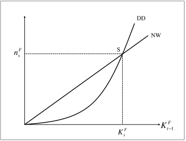
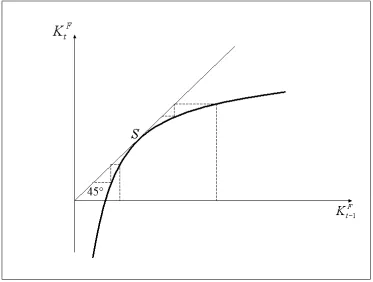
In order to compare our results with those obtained by KM we recall that in a real KM economy tKtF = KtF1; i.e. tradable output is equal to the

downpayment, whereas t=G

0

KG

t =R, i.e. the downpayment is equal to the

discounted value of the marginal productivity of the gatherer’s land. Therefore G0

K KF t

R = K

F

t 1. The steady state is represented in …gure 1.

In a monetary KM economy such as the present one, the dynamic system obtained by the maximization problems of the farmer and the gatherer consists of equations (11), (20), (24) and the de…nition of the downpayment, which we rewrite for convenience of the reader:

8 > > > > <

> > > > :

tKtF = KtF1 gMmFt

G0

KG

t =R t

mF t =

1

gM(1 + ) +'

KF

t 1+G KtG1

t=qt

qt+1

R

Notice that the RHS of the …rst equation represents net worth. Substituting the third equation into the RHS of the …rst one we get:

nF

DD

NW

S

F t

K

F s

K

s

n

Figure 1: Steady state in KM’s framework

where

A:= gM

1

gM(1 + ) +'

= 1

(1 + ) + ' gM

is a polynomial of policy parameters: gM, ' and . It is easy to verify that

0< A <1 and thatAis increasing withgM and decreasing with'and .

Therefore, recalling that K=KF

t +KtG, the RHS of the …rst equation can

be expressed as a function ofKF

t 1 as follows:

nFt = KtF1 A G K KtF1 + KtF1 (26)

It is easy to see thatnF

t is an increasing convex function of KtF1. In fact:

dnF t

dKF t 1

= (1 A) +AG0

K KtF1 = +A G 0

K KtF1 >0

d2_nF t

d KF t 1

2 = AG

00

sinceG00

K KF t 1 <0.

Notice now thatnF

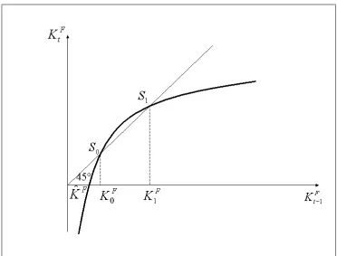
t = 0i¤yFt (1 A) =AyGt i.e. i¤:

h KtF1 :=

G K KF t 1

KF t 1

= 1

A 1 = 1 + ' gM

(27)

h KF

t 1 is the ratio of output of the gatherer to output of the farmer,h 0

<0. MoreoverlimKF

t ₁!0h K

F

t 1 = +1andh K =

G(0) K = 0.

( )

K h −1

F t

K

σ

ϕ









+

=

−

1

1

1

g

A

σ

ϕ









+

=

−

1

1

1

g

A

K

K

H

J

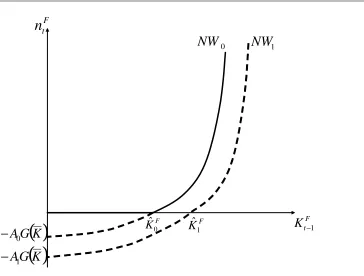
Figure 2: Determination ofK^F

Solving (27) forKF

t 1yields athreshold level of KtF1, sayK^F =h 1

(1 A) A such that ifKF

t 1 <K^F, thennFt <0 and the farmer goes bankrupt. We will

deal therefore only with the caseKF

t 1 > K^F. In particular this threshold is

a function of the policy parameters ' and gM. The determination of K^F is

represented in …g. 2. It is immediate to conclude that an expansionary policy move – for instance an increase ofgM – increases the threshold K^F (compare

F t

n

F t

K

K

F

K

0

NW

NW

( )

K

G

A

−

( )

K

G

A

−

Figure 3: The farmer’s net worth

In …gure 3 net worth is represented as a function of the farmer’s landholding according to equation (26). This graph shows the new shape of the Net Worth (NW) curve in a monetary KM economy. There are three di¤erences with respect to the NW curve in a real KM economy represented by the straight line of equationaKF

t 1 which represents tradable output.

First, the curve crosses the x-axis atK^F _{instead of the origin. This means}

that net worth becomes negative (a condition for bankruptcy) when “too much land” is in the hand of the gatherer. We focus on the case of solvent farmers and therefore rule out the dashed portion of the NW curve. Second, a nominal shock can a¤ect the position on the plane of the curve. In particular a monetary injection shifts the curve down. On the contrary, by construction, a nominal shock has no e¤ect on the NW schedule in a real KM economy. Third, in a monetary economy the NW curve undergoes a “convexi…cation”. This is due to the fact that also the gatherer’s production indirectly a¤ects the farmer’s net worth through the money market. An expansionary policy move – for instance an increase of gM – which makesA go up has also the e¤ect of increasing the

slope of the NW curve ifG0

> and of reducing it ifG0

< . The slope remains the same inG0

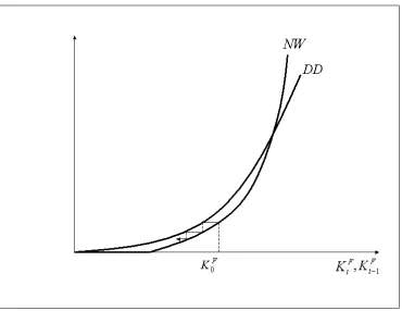
Figure 4: The DD-NW diagram. The case of a unique unstable steady state.

On the other hand the DD curve, which represents total downpayment _tKF t

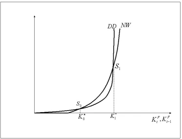
is exactly the same as in KM. Therefore we can envisage three scenarios. In the …rst one there is no intersection between the two curves (not shown). In the second one there is one intersection between the two curves (as shown in …gure 4). It is easy to see that the steady state is unstable. Finally the third and most interesting case is represented in …gure 5 where the NW curve intersects the DD curve twice. It is easy to reach the conclusion that the equilibriumS1

is stable whileS0 is unstable.

Substituting the second and the third equations of the dynamic system into the …rst one we get:

G0

K KF t

R K

F

t = KtF1(1 A) AG K KtF1 = (28)

= KF

t 1 A G K KtF1 + KtF1

Substituting the fourth equation into the second one and adapting the time index we get:

qt=Rqt 1 G 0

Figure 5: The DD-NW diagram. Multiple equilibria.

We end up therefore with the system (28) (29) of two non linear di¤erence equations in the state variables KF

t and qt. The system is recursive. The

dynamics ofKF

t in fact, is independent of the dynamics ofqt.

Let’s focus on (28) …rst. It is a …rst order non-linear di¤erence equation in Kt. In order to study the properties of the steady state, at least qualitatively, we

have to sketch the phase diagram. Applying the implicit function di¤erentiation theorem to:

f KtF; KtF1 =G 0

(K KtF)KtF KtF1R(1 A) +RAG K KtF1 = 0

which is another way of writing (28) we obtain:

dKF t

dKF t 1

=R +A G

0 _{K K}F t 1

G00_{(K K}F

t )KtF+G0(K KtF)

Notice now that:

"t=

G00

(K KF t )KtF

G0_{(K K}F t )

= @G

0

(K KF t )

@KF t

KF t

is the (non-negative) elasticity of the marginal productivity of the land of the gatherer with respect to the land of the farmer. Hence the slope of the phase diagram is:

dKF t

dKF t 1

=R +A G

0

K KF t 1

("t+ 1)G0(K KtF)

>0 (30)

Notice also that when KF

t ! K, G

0

(0) ! 1, thanks to one of Inada’s conditions. Moreover elasticity tends to"_K = G

00_(0)K

G0₍₀₎ = 0. Hence:

dKF t

dKF t 1

KF

t=K = 0

It is straightforward to conclude therefore that the phase diagram of (28) is increasing and concave (see …g. 7).

The phase diagram of (28) is reminiscent of the analogous phase diagram derived in the original KM case. At a glance the major qualitative di¤erence is the fact that the origin is not belonging to the phase diagram any more. The introduction of real money balances into the model leads to a “shift” downward of the phase diagram that now cuts the x-axis with a positive interceptKF

t 1=

^ KF_.

In a sense this is obvious because in the present context the farmer devotes part of his resources (consisting of output and credit) to money holdings. For each level of land inherited from the past, therefore, the amount of new land he can buy is smaller than in the original KM case.

Once again in the present context we can envisage three scenario. The phase diagram may not cross the45 line at all, may be tangent or may cross the45 line twice. In the …rst case there are no steady states (not shown). If the phase diagram is tangent to the45 line, trajectories starting from initial conditions above (below) the steady state S, converge to the steady state (diverge) (see …g. 6). Finally in the third case there are two steady states (see …g. 7).

We have only one steady state if the45 line is tangent to the phase diagram. This occurs if KF

t 1 =KtF = KsF, where KsF is the unique steady state, and

simultaneously the slope of the phase diagram is equal to1. This is the case i¤:

A= ^A:= R G

0 _{K K}F

s ("s+ 1)

R G0 _{K K}F s

5.1

Multiple equilibria

Let’s assume now that:

Figure 6: Phase diagram. The case of a unique steady state

Let’s go back now to the system (28) (29). In the steady stateKF

t 1=KtF =

KF _andq

t 1=qt=q so that equation (29) becomes:

q=G

0

K KF

R 1 (31)

(31) is the steady stateasset price equation. It establishes a positive link be-tween the farmer’s landholdings and the price of landin the steady state.

Notice now that in the steady state =q where = 1 1

R. Therefore (28) becomes:

q= (1 A) Ah KF _{= 1 A h K}F _{+ 1 (32)}

whereh KF ₌G K K F

KF ;h

0

KF _{<0 (see above).}

Figure 7: Phase Diagram: the case of multiple equilibria.

price as the sum of the discounted marginal productivities of the gatherer’s land (uniform across periods in the steady state) over an in…nite horizon. The higher KF_{, in the steady state, the lower K}G _{= K K}F_{, the higher the marginal}

productivity and therefore the price of landq.

The “story” one can tell to give the economic intuition of (31) is less straight-forward. One interpretation is as follows. The higherq, the higher the downpay-ment =q will be, the smaller should be therefore the amount of resources the farmer devotes to money holdings mF_{. In equilibrium, a smaller money}

holding is brought about by a higher landholdingKF_.

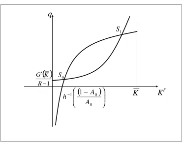
In order to study the steady state, let’s consider the system (31) and (32) which we rewrite here for convenience of the reader

8 > <

> :

q= G

0

K KF

R 1

q= (1 A) Ah KF (33)

andKF_{. It crosses the x-axis whenK}F _=h 1 (1 A)

A = ^K

F_{. IfK}F _!0

then q! 1, while if KF _{=K then q = (1 A). Therefore we conclude}

that, in the domain of interest, the second equation yields an increasing and concave relationship betweenq andKF_{. On the other hand, the …rst equation}

yields an increasing and convex relationship betweenqandKF _{on the K}F_{; q}

plane. It crosses the y-axis whenq= G

0

K

R 1 . When K

F _{!Kthenq! 1.}

q

F

K

( )

1

−

′

R

K

G

S

1

S

K

(

)







 −

−

0 0 1

1

A

A

h

Figure 8: Steady state loci

We can explore di¤erent scenarios. In fact, given the properties of the two relations above we can obtain one, two or no steady states depending on the level of the policy parameter (A). Thanks to assumption A1 we focus only on the case of multiple steady states (see …g. 8).4

In order to assess the properties of each of the two steady states, we linearize

4_{In order to obtain a closed form solution for the steady state we should specify the}

the system (33) around each steady state and compute the jacobian matrix:

Ji =

" _{R(1 A)+RAG}0_{(K K}F i)

("i+1)G0(K K F

i ) 0

G00

K KF

i R

#

(34)

withi= 0;1.

Ji is a lower triangular matrix. Therefore the eigenvalues coincide with the

elements on the main diagonal. One of the eigenvalues isR >1. The second eigenvalue R(1 A) +RAG

0

K KF i

("i+ 1)G

0_{(K K}F i )

coincides with the slope of the phase diagram of (28) in the steady state. In particular we observe that the slope is greater than one in the lower steady state S0 (i= 0) while it is smaller than

one in the higher steady stateS1 (i= 1). In the latter case therefore the steady

state is a saddle point. This means that there is only one trajectory on the KF

t ; qt phase space which is converging to the steady stateS1, i.e. the saddle

path. All the other trajectories diverge.

Figure 9: E¤ects of an expansionary monetary policy when the initial condition isS1

In …g. 9 the convex solid line represents equation (31), that is independent from A. The concave solid line represents equation (32). Let’s assume that the economy lies in the higher steady state (S1). Suppose that an expansionary

monetary policy increasesA. The concave curve shifts down: the new situation is represented by the dotted line. Assuming that qt jumps down to the new

saddle path, the economy follows a trajectory which converges to the new saddle point (S10). In other words in the end an increase of the rate of growth of the

money supply yields a decrease of the farmer’s landholding and of the asset price.

5.2

Net worth, money balances and the in‡ation tax

Notice that “in the long run” gM = , i.e. a change in the rate of growth

of money supply translates into a change in the rate of in‡ation of the same magnitude. Therefore the long run impact of the monetary expansion on the real price of land can be attributed toan in‡ation tax e¤ect.

In order to assess the overall impact of the policy move, we recall that aggregate output is de…ned as Yt = f KtF1 where f KtF1 = KtF1 +

G K KF

t 1 . Therefore aggregate output is a non monotonic function of the

farmer’s landholding. In particular it is easy to conclude thatYtis an increasing

(resp. decreasing) function ofKF

t 1if > G 0

K KF _{( < G}0

K KF _{). In}

other wordsYtis an increasing (resp. decreasing) function ofKtF1ifKtF1< KfF

(KF

t 1> KfF) whereKfF =K G

0 1_{( )is the farmer’s landholding which}

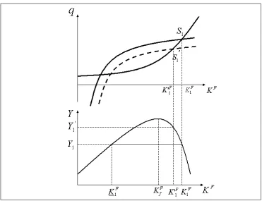
max-imizes aggregate output. In the case of the higher steady state,Y1=f K1F

Proposition 1 Starting fromS1, so thatKtF1=KtF =K1F andY1=f K1F , an expansionary policy move (i.e. an increase ofA due to an increase of the rate of growth of the money supply) has a positive long run e¤ect on aggregate output i¤KF

1 > KfF andK F

1 < K

0_F

1 < K1F, where KF1 is such thatf KF1 =

f KF

1 . On the other hand an expansionary policy move has a negative e¤ect on aggregate output i¤KF

1 > KfF andK 0_F

1 < KF1 or i¤K1F KfF 8K 0_F

1 .

In …gure 10 we represent the e¤ects of an expansionary policy move in the case with KF

1 > KfF and K F

1 < K

0_F

1 < K1F. As claimed in the proposition

above an increase of the rate of growth of money supply – i.e. an increase of the in‡ation tax – has a positive e¤ect on aggregate output. This counterintuitive result is due to the fact that following the decrease in the steady state farmer’s landholding fromKF

1 to K

0_F

1 , the economy moves along the downword sloping

branch of the aggregate output function: The loss of output due to the reduction in farmer’s landholding is more than o¤set by the increase of output due to the increase of the gatherer’s landholding.

Figure 10: Positive e¤ect of an expansionary policy move on aggregate output.

6

The e¤ects of an unexpected productivity shock

In this section, following the original KM approach we analyze the e¤ects of a small unexpected and temporary shock to technology on output and asset prices by means of a linear approximation around the saddle point.

Suppose that at time0the economy is in the saddle point and an unexpected technological shock occurs so that the productivity of the farmer increases from

0to 1. As in KM we assume that the farmer decides whether to supply labour

or not before the shock. If the farmer chooses to cultivate land, when the shock occurs it is too late to change his mind.Moreover the shock is temporary, i.e. the parameter goes back to 0 immediately after the shock.

In order to study the e¤ects of a shock to productivity, we start from the de…nition of net worth, i.e. the sum of tradable output KF

t 1 and thecurrent

value of real assets qtKtF1 net of interest payments RbFt 1 and of (a multiple

of) the increase in real money balances( gMmFt):

nF

t = ( +qt)KtF1 Rbt 1 gMmFt

Net worth is employed as downpayment, i.e. nF

Figure 11: Negative e¤ect of an expansionary policy move on aggregate output

G0

K KF

t and mFt =

1

gM(1 + ) +'

KF

t 1+G KtG1 :Therefore:

G0

K KF t

R K

F

t = [ (1 A) +qt]KtF1 AG K KtF1 Rbt 1 (35)

At time0, before the shock,nF

0 = 0(1 A)K0F+q0K0F Rb0 AG K K0F

andq0K0F =Rb0– i.e. the current value of the farmer’s land is equal to interest

payments on debt inherited from the past – so that (35) boils down to:

G0

K KF

0

R K

F

0 = (1 A) 0K0F AG K K0F (36)

Suppose now that in the same period the productivity parameter goes up by = 1 0. By assumption, the …rst round e¤ect of the shock on net

worth concerns tradable output and the price of land,given the (steady state) landholding of the farmer KF

0. Immediately after the shock, net worth becomes

nF

since interest payments have been predetermined on the basis of the steady state price of land: q0K0F =Rb0:The …rst round e¤ect of the shock creates a wedge

between the current (after shock) value of land qtK0F and interest payments

q0K0F. In particular, as will be clear in the following, the current price of land jumpsfrom q0 toqtcreating an (unexpected)capital gain.

Substituting (37) into the RHS of (35) we obtain G0 _{K K}F

t

R K

F

t = [( 0+ ) (1 A) + (qt q0)]K0F AG K K0F (38)

which describes the impact of the shock onKF t .

Assuming that the shock is temporary, in period 1 and all the following periods the situation goes “back to normal”, i.e.

nFt+s= 0(1 A)KtF+s 1 AG K KtF+s 1 =

G0

K KF t+s

R K

F

t+s s= 0;1; :::

(39) Consider now (38). Let’s take a …rst order approximation of the LHS inKF

0:

G0

K KF t

R K

F t

G0

K KF

0

R K

F

0 +

G0

K KF

0

R ("0+ 1) K

F t K0F

(40) where:

"0=

G00

K KF

0 K0F

G0 _{K K}F

0

K0F

is the elasticity of the marginal productivity of the land of the gatherer with respect to the land of the farmerevaluated in the steady state KF

0.

The rate of change of total downpayment, i.e. of the LHS of (40), relative to the steady state is

"

G0

K KF t

R K

F t =

G0

K KF

0

R K

F

0

#

1. Denoting the

rate of change of a variable with respect to the steady state with a hat, the rate of change of the LHS becomes:

\

tKtF = ("0+ 1) ^KtF (41)

whereK^F t =

KF t K0F

KF

0

is the rate of change of the farmer’s landholding. On the other hand, the rate of change of net worth, i.e. of the RHS of (38), is [( 0+ ) (1 A) + (qt q0)]K0F AG K K0F

0(1 A)K0F AG K K0F

1. Butq0 1 1

R K0=

0K0=

G0 _{K K}F

0

R K0= 0(1 A)K

F

0 AG K K0F so that the rate of

change of the RHS becomes:

^ nF

AS = ^ (1 A)

0

q0

R R 1+ ^qt

R

where^ = a0

andq^t=

qt q0

q0

are the rates of change of the farmer’s produc-tivity and of the price of land.

After the productivity shock, the farmer’s net worth goes up for two reasons: the direct e¤ect ^ (1 A) 0

q0

R

R 1 and theindirect e¤ect through asset prices ^

qt

R

R 1. Notice that 0 < A < 1. Moreover in our context, as stated in (12)

0 =q0

R 1

R < 0: Hence the ratio of the productivity to the downpayment

0

q0

R

R 1 ,which we will denote with 0in the following, is greater than one. In symbols 0:= 0

q0

R R 1 >1:

In the original KM framework the rate of change of the farmer’s net worth is ^

nF

AS= ^ + ^qt

R

R 1. From a comparison with (42) it is clear that in the present model the indirect e¤ect is speci…ed exactly as in KM while the direct e¤ect ^ (1 A) 0 is greater than^ (as in KM) ifA <1

1

0. The smaller the policy

parameterA, the higher the direct e¤ect of the productivity shock on the rate of change of net worth after the shock.

Equating (41) and (42) we get

("0+ 1) ^KtF = ^ (1 A) 0+ ^qt

R

R 1 (43)

We have to determine now how the asset priceqtchanges over time.

Follow-ing KM, we note that from the de…nition of the downpayment and (20) follows qt =

G0 _{K K}F t

R +

qt+1

R , qt+1 =

G0 _{K K}F t+1

R +

qt+2

R and so on. Substi-tuting the second expression in the …rst one and iterating the procedure we end up with:

qt=

G0

K KF t

R +

G0

K KF t+1

R2 +:::= 1

X

s=0

R sG

0

K KF t+s

R (44)

i.e. the current price of land is equal to the present value of the stream of future downpayments over an in…nite horizon.

Taking a …rst order approximation of G0

K KF

t+s in K0F, we can write

G0

K KF t+s G

0

K KF

0 G

00

K KF

0 KtF+s K0F . Noting that this

approximation holds true for any time periods, equation (44) boils down to:

qt=

1

X

s=0

R sG

0 _{K K}F

0 G00 K K0F KtF+s K0F

R

Recalling thatP1_s=0R s=

R

R 1 and that G0

K KF

0

R =q0 R 1

expression above we obtain:

^ qt=

1 q0

G00

K KF

0

R

1

X

s=0

R s _KF

t+s K0F

Notice now that 1 q0

G00

K KF

0

R =

G00

K KF

0

G0 _{K K}F

0 R 1 R = "0 KF 0 R 1 R . MoreoverP1

s=0R sK0F =K0F

R

R 1. Thereforeq^t="0 R 1

R

P1

s=0R sK^tF+s.

In the end we obtain:

^ qt="0

R 1 R

1

X

s=0

R s 1

"0+ 1

s

^ KF

t

MoreoverP1_s=0R s 1

"0+ 1

s

=P1_s=0 1 R("0+ 1)

s

= R("0+ 1) R("0+ 1) 1

. There-fore

^

qt="0(R 1) ("0+ 1)

R("0+ 1) 1

^

KtF (45)

Solving (43) and (45) forq^t andK^tF yields

^

qt="0(1 A) 0^ (46)

^ KtF =

R("0+ 1) 1

(R 1) ("0+ 1)

(1 A) 0^ (47)

The rate of change of net worth^nF

AS= (1 A) 0 1 +

R

R 1"0 ^is larger than the rate of growth of productivity thanks to the indirect e¤ect of the shock on the price of land. The rate of change of total downpayment ("0+ 1) ^KtF

should match to keep equilibrium on the market for land. Therefore the rate of change of landholding is a multiple of the rate of change of productivity. In fact the multiplier 1

"0+ 1

1 + R

R 1"0 is greater than one.

7

The e¤ects of an unexpected monetary shock

In this section we analyze the e¤ects of a small shock to the rate of growth of money supply on output and asset prices by means of a linear approximation around the saddle point. Suppose that at time 0 the economy is in a steady state and an unexpected increase of the rate of growth of money supply makes Aincrease from A0 to A1. Assume moreover that the shock is temporary, i.e.

the parameterAgoes back toA0 immediately after the shock.

By assumption, the …rst round e¤ect of the shock on net worth concerns the price of land,given the (steady state) landholding of the farmer KF

0.

Immedi-ately after the shock, denoting with A=A1 A0, net worth becomes

nF

Since interest payments have been predetermined on the basis of the steady state price of land (q0K0F =RbF0 ) we can write:

G0

K KF t

R K

F

t = (1 A0 A)K0F A0G K K0F AG K K0F +(qt q0)K0F

The rate of change of net worth, i.e. of the RHS, is:

^ nF

AS = ( 0 1) ^A+ ^qt

R

R 1 (48)

whereA^= A A0

and 0:= 0

q0

R R 1 >1.

After the shock, the farmer’s net worth changes for two reasons: the direct e¤ect of the rate of growth of money supply ( 0 1) ^Aand the indirect e¤ect

of the rate of growth of money supply on net worththrough asset pricesq^t

R R 1. This indirect e¤ect is a multiple R

R 1 of the asset price increase. The direct e¤ect of the rate of growth of money supply is negative.

Equating (41) and (48) we get:

("0+ 1) ^KtF = ( 0 1) ^A+ ^qt

R

R 1 (49)

Solving (49) and (45) forq^tandK^tF yields:

^

qt= ( 0 1) ^A

^ KF

t = ( 0 1)

R("0+ 1) 1

(R 1) ("0+ 1)

^ A

An increase in the rate of change of money supply, has negative e¤ects both on the rate of change of the farmer’s landholding and the rate of change of the asset price. The rate of change of net worth in the end isn^F

AS = ( 0 1) ^A

2R 1 R 1 .

8

Conclusions

In this paper we have developed a model of a monetary economy with …nancing constraints. We borrow some of the basic ingredients of Kiyotaki and Moore’s …nancial accelerator framework in order to keep the appealing feature of the intertwined dynamics of asset price changes and borrowing constraints. In or-der to evaluate the impact of monetary policy, however, we model a monetary economy with …nancing constraints adopting the Money In the Utility function (MIU) approach.

References

[1] Bernanke, B. and Gertler, M . (1989), “Agency Costs, Net Worth and Business Fluctuations”, American Economic Review, vol. 79, pp. 14-31. [2] Bernanke, B. and Gertler, M. (1990), “Financial Fragility and Economic

Performance”,Quarterly Journal of Economics, vol. 105, pp. 87-114. [3] Bernanke, B., Gertler, M. and Gilchrist, S. (1999), “The Financial

Acceler-ator in Quantitative Business Cycle Framework”, in Taylor, J. e Woodford, M. (eds), Handbook of Macroeconomics, vol 1C, North Holland, Amster-dam.

[4] Cordoba, J. C., Ripoll, M. (2004a) “Collateral Constraints in a Monetary Economy” Journal of the European Economic Association, vol. 2, no. 6, pp. 1172-1205.

[5] Cordoba, J. C., Ripoll, M. (2004b) “Credit Cycles Redux” International Economic Review vol. 45, no. 4.

[6] Cooley, T. and Hansen, G. (1998) “The Role of Monetary Shocks in Equi-librium Business Cycle Theory: Three Examples,”European Economic Re-view vol. 42, pp. 605-617.

[7] Iacoviello, M. (2005a) “House Prices, Borrowing Constraints and Monetary Policy in the Business Cycles” The American Economic Review, vol. 95, no. 3, pp. 739-764(26).

[8] Kiyotaki, N. (1998) “Credit and Business Cycles”The Japanese Economic Review, vol. 49, no. 1.

[9] Kiyotaki, N. and Moore, J. (1997), “Credit Cycles”, Journal of Political Economy, vol. 105, pp.211-248.

[10] Kiyotaki, N. and Moore, J. (2002a), “Balance-Sheet Contagion,”American Economic Review, vol. 92(2), pp. 46-50.

[11] Kiyotaki, N. and Moore, J. (2002b), “Evil is the Root of all Money”, Amer-ican Economic Review, vol. 92(2), pp. 62-66.