New Housing Supply and the Dilution of Social Capital

Munich Personal RePEc Archive

New Housing Supply and the Dilution of

Social Capital

Hilber, Christian A. L.

London School of Economics

2 August 2007

Online at

https://mpra.ub.uni-muenchen.de/5134/

Research Papers in Environmental and Spatial Analysis No. 123

NEW HOUSING SUPPLY

AND THE

DILUTION OF SOCIAL CAPITAL

by

Christian A. L. Hilber

∗

Department of Geography and Environment

London School of Economics

August 2007

ISBN: 978-0-85328-114-6

∗ _{The author wishes to thank Paul Cheshire, Gilles Duranton, Steve Gibbons, Edward Norton, Jos Van}

Research Papers in Environmental and Spatial Analysis No. 123

NEW HOUSING SUPPLY

AND THE

DILUTION OF SOCIAL CAPITAL

Abstract

This paper examines the role of local housing market conditions for social capital

accumulation and neighborhood club good provision. A model of individual investment

decisions predicts that in a setting with high property transaction costs (i) homeowners are

more likely to invest in social capital than renters and (ii) the positive link between

homeownership and social capital is stronger in more built-up neighborhoods with inelastic

supply of new housing. In these neighborhoods homeowners are largely protected from

inflows of newcomers that would dilute the net benefit from social capital in the longer run.

Empirical evidence from the Social Capital Community Benchmark Survey confirms the

model predictions. Instrumental variable estimates suggest that the effects are causal.

JEL classification: D71, R21, R31.

Keywords: House price capitalization, social capital, homeownership,

1 Introduction and Background

The monitoring of one’s property by friendly neighbors or watch groups, a neighbor

holding one’s spare key, BBQ-parties among closely connected neighbors, or a pool of

trusting parents that look after each other’s children are all examples of club goods that are

essentially the result of accumulated social capital among a group of contributing neighbors.

In this context, DiPasquale and Glaeser (1999) have argued that homeowners are ‘better

citizens’ because homeownership (i) creates barriers to mobility and (ii) gives individuals an

incentive to invest in local amenities and social capital since community quality is capitalized

into property values.

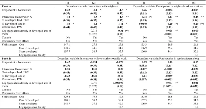
Simple stylized facts from the Social Capital Community Benchmark Survey (2000),

suggest, however, that homeowners may not always be ‘better citizens’. For example, while

homeowners, compared to renters, on average socially interact 30 percent more often with

immediate neighbors in essentially built-up neighborhoods (more than 85 percent developed),

the difference between the two groups is only about 9 percent in an ‘average’ neighborhood

(45 to 55 percent developed) and there is virtually no difference between the two groups in

little developed neighborhoods (less than 15 percent developed). These numbers change little

when other factors – including population density in the developed area – are controlled for.

How can this be explained? In this paper I argue that property transaction costs

(interpreted broadly) create incentives for homeowners to invest in social capital because it

discourages free riding. Homeowners can in principle free ride on other neighbors’ social

capital investments by selling their property and pocketing the proceeds from the improved

neighborhood quality. However, such free riding is not an attractive option if transaction costs

exceed the benefits derived from the improved neighborhood quality. In a world with high

transaction costs the question then becomes whether the homeowner’s long-term benefits

derived from social capital exceed the costs and I will argue that the answer to this question

crucially depends on the elasticity of new local housing supply – proxied by the share of

developable land in the neighborhood.

Consider a neighborhood where renters are free to move but where property transaction

costs make existing homeowners immobile. In such a setting homeowners have greater

incentives to invest in social capital compared to renters as long as the long-term net benefit

exceeds the initial investment cost. This is because homeowners can internalize the long-term

net benefits from their investments. In contrast, renters are deprived of those net benefits since

critical for the likelihood of social capital investment because it affects the inflow of

newcomers and thereby determines the homeowners’ long-term net benefit from social

capital. In a built-up neighborhood with perfectly inelastic supply of developable land for new

housing, initial investors into social capital are largely protected from inflows of newcomers

that would dilute the net benefit from that social capital in the longer run.1 In contrast, in a

little developed neighborhood with elastic supply (i.e., low opportunity cost of conversion and

lax land use regulations), newly accumulated social capital will steer landowners to develop

new housing units as long as the price exceeds the marginal (opportunity) cost of conversion.

In the long-run, the net benefit from social capital is diluted to an extent that the marginal

newcomer’s net benefit and the corresponding house price premium become very small. It is

quite intuitive that in such a setting nobody has an incentive to make a sizeable investment in

the neighborhood’s social capital in the first place. Hence, homeowners may only be ‘better

citizens’ in more built-up neighborhoods with inelastic long-term supply of new housing.

The outlined argument is not only relevant for investment in social capital. For example,

an investment in a local public school may increase school quality in the short-run. However,

if supply of new housing is elastic, inflow of households with children will dilute the benefits

in the longer-run (because the additional resources have to be shared among more pupils) and

thereby reduce the homeowner’s incentive to vote for the investment in the first place. Hilber

and Mayer (2004) provide empirical evidence that is consistent with this view.

In an even broader context, the outlined argument is important for a wide range of studies

that conclude that homeowners are ‘better citizens’ or are ‘more motivated to control local

government because its services and taxes affect the value of their homes’ (e.g., DiPasquale

and Glaeser, 1999; Fischel, 2001), that house value maximizing voters can ensure an efficient

provision of local public services (see e.g. Edelson, 1976; Sonstelie and Portney, 1978;

Wildasin, 1979; Sprunger and Wilson, 1998), or that house price capitalization provides an

incentive mechanism in an inter-temporal sense, that is, an incentive to provide an optimal

level of durable or intergenerational public goods (see e.g. Brueckner and Joo, 1991; Glaeser,

1996; Oates and Schwab, 1996 and 1998; Conley and Rangel, 2001; Rangel, 2005).

The empirical evidence presented in this paper provides strong support for the view that

in a world with high transaction costs the elasticity of new housing supply – as proxied by the

1

share of developable land in the neighborhood – is an important determinant of a household’s

social capital investment decision. This is true even when controlling for the population

density within the developed area of the neighborhood and many other characteristics that are

expected to affect social capital accumulation and even when using instrumental variable (IV)

estimates that treat the share developed land, the population density and the respondent’s

homeownership status as endogenous.2 The empirical analysis also tests and confirms other

elements of the theory and discounts alternative explanations of the empirical findings.

The paper is structured as follows. Section 2 describes the economic characteristics of

neighborhood specific social capital, presents a two-stage model of individual investment

decisions and discusses alternative theoretical frameworks and their predictions. Section 3

describes the data sources, discusses empirical specifications and identification strategies and

presents evidence in support of the model predictions. Section 4 derives conclusions.

2 Theoretical Framework and Predictions

2.1 Economic Characteristics of Neighborhood Specific Social Capital

Neighborhood specific social capital is defined in this paper as a connection among

neighbors, which enables them to cooperate and which subsequently facilitates the provision

of a number of mutually beneficial club goods.3 Neighborhood specific social capital can be

accumulated, for example, by socially interacting with neighbors or by participating in

neighborhood clubs. These activities enable individuals to (a) develop a common language

with one another so that communication is easier and (b) establish relationships, for example,

in the form of organized or spontaneous shared social activities, so that neighbors will trust

and like each other more. While shared social activities (e.g., BBQ-parties among neighbors)

themselves can be interpreted as utility generating club goods, other club goods are the result

of social capital induced trust and friendship. For example, trust and sympathy among

neighbors enables them to provide club goods that are simply the product of shared private or

2

The empirical work below decomposes the population density in a neighborhood into two multiplicative components: the population density in the developed area and the share of developed land in the neigbhorhood. This approach enables separate estimation of the effect of land scarcity (potential supply of new housing) and the physical proximity of neighbors (as an inverse measure for the cost of social interactions). See Brueckner and Largey (2006) for an analysis of the effect of population density – measured as population divided by total area – on individual measures of social capital investment. Largely consistent with the findings in this paper, their empirical results show a negative rather than a positive effect of density on the number of social interactions.

3

common property (e.g., shared or communal gardens). Finally, trust and sympathy can

encourage the provision of benefits in the form of mutually beneficial reciprocal behavior

(e.g., monitoring of one’s absent property by friendly neighbors, holding a neighbor’s spare

key, or informal child care arrangements).

Neighborhood specific social capital has some particular economic characteristics. To

begin with, it is in practice partially but not fully excludable. Investors in neighborhood

specific social capital (‘club members’) can typically exclude free riders from access to the

benefits derived from social capital, for example, by not inviting them to join a club event or

by turning a blind eye on an absent free rider’s property. However, exclusion is in practice

incomplete in that it is often unfeasible, not considered fair or in some cases not rational to

exclude newcomers to a neighborhood who are willing to cooperate. One consequence of this

partial non-excludability is that net benefits derived from neighborhood specific social capital,

after an initial investment period, make the location not only more attractive to existing

residents but also to potential newcomers, increasing the demand for properties in the

neighborhood, and – assuming that housing supply is not perfectly elastic – also increasing

house values.4 This implies that property owners can free ride on other residents’ investments

by selling their property as long as the potential gains exceed property transaction costs.

Another defining characteristic of neighborhood specific social capital is that it typically

involves an initial investment/production phase and a subsequent maintenance/consumption

phase. Consider the investment phase first. A quite sizeable ‘social capital investment’ is

usually needed to initiate the process of generating trust and friendship among the involved

neighbors M . The individual investment costs of contributing neighbors can be expressed as

[ ]

f

[ ]

+ v

[ ]

inv inv inv

c M =c M c M . (1)

The term f inv

c denotes each initiating member’s share of the total fixed cost burden f inv

C

associated with the set up of initiating meetings and club structures, whereas f f inv inv

c =C M

(i.e., the fixed cost is shared equally among all members). The term v inv

c denotes the individual variable cost related to the time spent to establish relationships with all involved initiating club members. It can be assumed that this cost component increases linearly with M (i.e., there are no economies of scales in establishing trust). First and second derivatives yield:

4

2 2 2 2 2 2 0 0 ; 0

; = ; 0

0 ; 0 0

f v

f f

inv inv inv inv

inv inv

v v f v

inv inv inv inv

c c

c c

if

M M

M M _{c c}

M M

c c c c

if

M M M M

 _{∂ ∂}

∂ _< ∂ _{> < >}

 ∂ ∂ ∂ ∂ ∂  ∂ >  ∂ ∂

∂ _> ∂ ₌ _> ∂ _<∂



∂ ∂  ∂ ∂

(1.1)

The last two derivatives imply that the individual social capital investment cost first

decreases and then increases with the number of initiating investors (inverse U-shaped curve).

Now consider the maintenance phase. Once trust and friendship among initiating

investors is established, a ‘maintenance effort’ of ‘contributors’ (initial investors and

cooperative newcomers) is usually sufficient to ensure the provision of social capital induced

club benefits in the longer run. The individual maintenance costs are determined by (a) the

number of initial club members M (the larger the club size the more relationships need to be maintained among initiating members) and (b) the number of cooperative newcomers ∆M

(new relationships need to be established). In this context it is reasonable to assume that the

cost of maintaining an existing relationship λexist

is significantly lower than the cost of

establishing a new relationship λnew

. Newcomers have to establish relationships with all club members, while initiating club members only have to establish relationships with the

newcomers. The cost functions for initial investors and newcomers can be expressed as:

[

,

]

exist new inv

m M ∆M =M×

λ

+ ∆ ×M

λ

(2.1)

[

] [

]

new new

m M+ ∆M = M + ∆M ×

λ

.5 (2.2)

If we define

λ

new−

λ

exist = ∆ >

λ

( )

0

and reformulate equations (2.1) and (2.2) we get:

[ ]

[

]

[

,

]

new inv new inv

m ₋ M m M M m M M M

λ

∆ = + ∆ − ∆ = × ∆ , (2.3)

whereas 0< ∆mnew inv−

[ ]

M <cinv

[ ]

M .

6

Equation (2.3) implies that newcomers, compared to initial investors, have higher costs in

the maintenance phase and that the cost difference depends on the number of initiators in

period 1. Overall, however, newcomers have a comparative cost advantage over initiators for

5

Alternatively, one could assume that the marginal cost of establishing a new relationship increases because the involved neighbors have time constraints and because a large number of newcomers threatens the developed common language. This alternative assumption does not fundamentally alter the model predictions.

6

This follows from the fact that it is not plausible to assume that the cost of establishing a contact in the initiating phase exceeds the cost λnew

of establishing a new contact in the maintenance phase. If the

per-contact-cost are assumed to be identical (=λnew

) then

[ ]

f

inv inv

c M =C M+ ×M λ. Consequently, c_inv

[ ]

M -∆m_{new inv−}

[ ]

M

= f

(

)

0

inv

C M+M× − ∆ >λ λ , since λ_{− ∆ =}λ λexist _>0

and f 0

inv

two reasons: Firstly, newcomers avoid the fixed costs associated with the initiation process.

Secondly, newcomers only have to establish contacts with initiators in the maintenance phase,

while initiators have to establish and maintain those contacts.

Finally, the social capital induced gross benefits B can be assumed to increase at a decreasing rate with the number of club members M+ ∆M in the maintenance phase, that is,

(

)

0

B M M

∂ ∂ + ∆ > and ∂2B ∂

(

M + ∆M

)

2 <0. Take the example of childcare arrangements among trusting parents. Adding another mutually beneficial link to a small pool of parents

substantially increases the likelihood of being able to make an arrangement when needed.

Adding another link to a very large pool increases each member’s benefit only marginally.

2.2 A Model of Social Capital Investment Decisions

This section presents a model with individual social capital investment decisions that

explicates the provision of social capital induced benefits as the outcome of a dynamic game

with complete and perfect information and with a symmetric equilibrium in pure strategy.7

The model, which builds on the considerations in Section 2.1 and uses its notations, is

parsimonious in that it only consists of one neighborhood with some open developable land –

plus the outside world – and two time periods t∈

{ }

1, 2 ; an investment or production phase

(stage 1) and a subsequent maintenance and consumption phase (stage 2). The game is solved

backwards. The investment decisions are modeled as discrete functions.

Basic Structure and Assumptions

I start with a brief overview of the game, describing the timing, the set of players and

their set of actions. Then I formulate the players’ payoff-functions.

Stage 1:

1. Homeowners and renters in the neighborhood individually, simultaneously and

non-cooperatively choose whether to invest in social capital. The investment amount

[ ]

inv

c M depends on M , the number of initiating club members in stage 1, as discussed in the previous section. A household invests if the investment generates a positive payoff.

The social capital induced club good is provided if at least two households invest in

social capital in stage 1.

7

2. Homeowners and renters choose whether to stay or exit. If homeowners leave at the end

of stage 1 they face transaction costs TC_O but receive a social capital induced house price premium ∆ = −P

(

P₂ P₁

)

determined in the second stage. Relocation for renters is costless.

Stage 2:

3. Initial investors get access to the social capital induced benefits B conditional on bearing the maintenance costs m_inv

[

M,∆M

]

. (Under the assumption of perfect and complete information, no household has an incentive to invest in stage 1 if this does not ensure

access to social capital induced benefits in stage 2. Because the benefits are conditional

on the maintenance effort, all initial investors will bear the maintenance cost in stage 2.)

Non-investors in stage 1 are excluded from access to the benefits in the second stage. The

benefits B M

[

+ ∆M

]

depend on the number of club members in stage 2.

4. The owners of undeveloped land (and the owners of vacated housing units) observe the

investment and relocation decisions of the residents in stage 1 and then post their

reservation prices for converting their plots of land competitively in the second stage.

Each landowner individually chooses whether to develop. (The equilibrium price P₂ and the corresponding social capital induced house price premium ∆P are determined by the developer of the marginal plot of land. As will be demonstrated below, as long as new

housing supply is not perfectly inelastic, the social club good induced equilibrium price

premium is determined by the marginal owner of undeveloped land rather than by owners

of units that were vacated in stage 1 (i.e., landlords). Landlords can be considered to be

price takers. Their actions are not explicitly modeled without any loss of generality.)

5. Households outside the neighborhood observe the investment and relocation decisions in

stage 1. They then choose whether to enter the neighborhood and join the club.8 If they

enter they pay ∆P plus the social capital maintenance cost m_new

[

M+ ∆M

]

in order to get access to the social capital induced benefits B M

[

+ ∆M

]

. (Whether newcomers buy or rent in the last stage is immaterial because both options generate identical payoffs.)

Next, I make a number of further assumptions and impose structural form to reflect the

above characterization of neighborhood specific social capital and to keep the model tractable.

8

To begin with, the neighborhood is initially occupied by H₁ residents. Each household

{

1, ... , 1

}

h∈ H occupies exactly one housing unit of fixed size, for convenience set to 1.9 The neighborhood has a total area L and contains open developable land L−H₁. That is, the share of developed land in stage 1 is predetermined. The fractions

α

of homeowners and

1−α of renters in period 1 are predetermined as well.10 Apart from idiosyncratic differences

in the preferences for homeownership all residents in the neighborhood are identical. (This

simplifying assumption helps illustrating the difference between homeowners’ and renters’

investment incentives. It does so at the cost of generating an outcome in which all agents of

the same group take the same action; invest or not invest. Alternative assumptions generate

more refined outcomes but do not fundamentally alter the propositions made in this paper.)11

The neighborhood is assumed to be sufficiently small such that it is not feasible to

replicate the social capital stock with membership levels that ensure positive payoffs. The

social capital induced benefits require social capital as sole ‘input factor in production’.

In line with the argumentation in Section 2.1, in stage 1 a substantial initial ‘social capital

investment’ cinv

[ ]

M is required from each of the M initial investors. In stage 2 a smaller

social capital ‘maintenance effort’ minv

[

M,∆M

]

is sufficient to maintain club membership.

Similarly, each cooperating newcomer has to pay m_new

[

M + ∆M

]

to ensure access to the club. Establishing new relationships is equally costly for initial investors and newcomers, however,

newcomers have to establish rather than just maintain relationships with initial investors. The

difference between the two cost functions is expressed in equation (2.3).

For expository purposes it is assumed that the social capital induced gross benefits B only accrue in stage 2. This simplifying assumption does not significantly alter the main

predictions of the model. It captures the idea that club benefits need to be produced through a

9

Existing homeowners in stage 1 are assumed only to own their own property and not parts of the undeveloped land in the neighborhood. That is, a homeowner bases the social capital investment decision solely on the social capital induced net benefits and on the value of the occupied property. Corporate or private owners of open land are assumed to be absent in that they do not have any direct influence on investment in social capital.

10

This is a reasonable assumption. The homeownership status of properties is in reality predetermined because different property types differ in their relative landlord production efficiency (Linneman, 1985) and different neighborhoods differ in their inherent investment risk (Hilber, 2005).

11

Alternatively one could assume that homeowners (and/or renters) differ in the benefits they enjoy from access to social capital, generating an equilibrium, in which agents of the same group take different actions. For example, the benefits could be uniformly distributed over an interval _0,B M

[

+ ∆M

]

_. B M

[

+ ∆M

]

follows the

process of social capital accumulation. The net benefits of initial investors and newcomers in stage 2 can be expressed as:

[

] [

]

[

]

2,inv , inv ,

NB M ∆M =B M + ∆M −m M ∆M (3.1)

[

] [

]

[

]

2,new new

NB M + ∆M =B M + ∆M −m M + ∆M . (3.2)

First and second derivatives yield:

(

2,inv

)

(

2,new

)

(

)

new

NB NB B

M M M M M M

λ

∂ ₌ ∂ ₌ ∂ ₋

∂ + ∆ ∂ + ∆ ∂ + ∆ (3.3)

(

)

(

)

(

)

2 2 2

2, 2,

2 2 2 0.

inv new

NB NB B

M M M M M M

∂ ₌ ∂ ₌ ∂ _<

∂ + ∆ ∂ + ∆ ∂ + ∆ (3.4)

Equations (3.3) and (3.4) imply that the net benefit functions of both investors and

newcomers are first increasing, then decreasing in the number of members in stage 2.

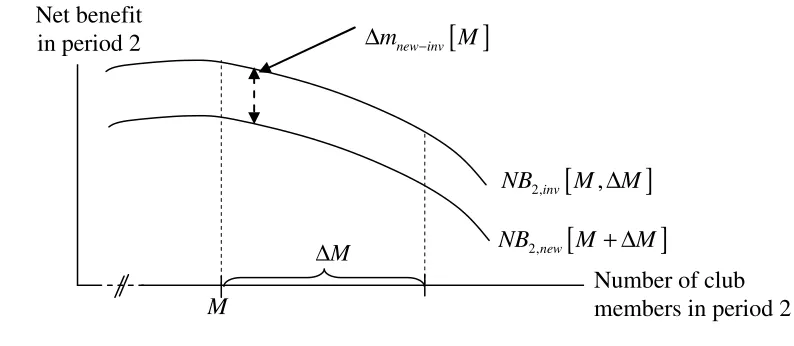
Combining equations (2.3), (3.1) and (3.2), the additional net benefit of an investor

compared to a newcomer in stage 2 can be formulated as:

[ ]

[

]

[

]

[ ]

2,inv new 2,inv , 2,new new inv

NB ₋ M NB M M NB M M m ₋ M

∆ = ∆ − + ∆ = ∆ . (4)

Figure 1 illustrates the net benefit functions for investors and newcomers. In the

illustrated case, at membership level M, even the first newcomer generates higher marginal

costs than marginal benefits. That is, newcomers to the neighborhood always dilute the club

[image:12.595.93.490.511.684.2]

good induced net benefit.12

Figure 1: Net Benefit as a Function of the Number of Newcomers in Stage 2

M

∆

[ ]

new inv

m ₋ M

∆

[

]

2,new

NB M + ∆M

[

]

2,inv , NB M ∆M

M

Number of club members in period 2 Net benefit

in period 2

12

Theoretically the first newcomers could increase the club good induced net benefits, as ∂ ∂B

(

M+ ∆M

)

may be greater than λnew

Relocation costs are in practice significantly higher for homeowners than for renters/

landlords. This is because relocation of a homeowner implies a property sale, while the

relocation of a renter does not involve such a transaction.13 For expository purposes it is

assumed that relocation of renters is costless for both renters and landlords but that

owner-occupiers face property transaction costs TC_O (e.g., search costs in the form of property advertising costs and estate agent fees, legal fees, and capital gains taxes).

Before any newcomer enters the neighborhood in stage 2, the provision of social capital

induced club goods is assumed to raise the hypothetically attainable utility level beyond that

of other neighborhoods in the economy. However, this encourages newcomers to enter,

decreasing the social capital induced net benefit NB_2,new

[

M + ∆M

]

(dilution effect due to maintenance cost increase), increasing demand for housing and increasing incentives of

landowners to convert open land into housing. 14

Each landowner l∈

{

1, ... ,L−H₁

}

is assumed to have a unique reservation price l t

P that determines whether the corresponding plot of land is converted into housing. The reservation

price is the result of individual opportunity cost considerations. Landowners with low

opportunity costs convert first, while landowners with high opportunity costs (for example

because of strong preferences for preservation) wait until the price exceeds their reservation

price. House prices Pt are assumed to be determined competitively such that in each stage

house prices equal the marginal landowner’s opportunity cost of conversion: P Ht

[ ]

t =

[ ]

. t t

MOC H Simple first differencing yields:

P MOC

∆ = ∆ , (5)

whereas ∆ =P P H₂

[ ] [ ]

₂ −P H_{1 1} and ∆MOC=MOC H₂

[ ]

₂ −MOC H₁

[ ]

₁ .

Finally, it is assumed that the marginal opportunity cost curve MOC H

( )

is more inelastic

in neighborhoods that are more developed, implying that

MOC MOC H L 

∆ = ∆ _{ } with

(

MOC

)

0.

H L

∂∆ _>

∂ (5.1)

13

Haurin and Gill (2002) estimate the transaction costs of selling a house in the United States as the sum of 3 percent of the house value and 4 percent of total household earning. This is likely a lower bound estimate of the true property transaction cost. In practice relocation costs of renters and landlords (i.e., search costs, short-term vacancy costs) are not zero but substantially lower than the property transaction costs faced by homeowners.

14

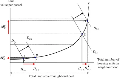
This alleged positive relationship between land scarcity and the inelasticity of new housing supply is both theoretically and empirically motivated and is further justified in

Section 3.2. Appendix Figure A1 provides a graphical illustration of the argument.

Payoff Functions

Under the above assumptions we can express the payoffs of homeowners h O

π , renters h R

π ,

landowners πLl and newcomers n N

π as follows:

(

1

)

2,

(

1

)

1 1

h h

inv h h inv

R

R NB R P

I c

r r

π

= − + − − − ∆

+ +

 

 

(6.1)

(

1

)

2,

1 1

h

inv

h h inv h O

O

R NB _{P TC}

I c R

r r

π

= − + − + ∆ −

+ +

 

 

(6.2)

{

2 2

}

l l l

L D P P

π = − (6.3)

{

2,

}

n n

N E NB new P

π = − ∆ , (6.4)

whereas r denotes the discount rate, h

{ }

0,1

I ∈ and h

{ }

0,1

R ∈ denote the choices of

household h whether to invest in social capital and whether to relocate at the end of stage 1,

{ }

0,1 l

D ∈ denotes the choice of landowner l whether to convert the open plot of land into housing, n

{ }

0,1

E ∈ denotes the choice of newcomer n whether to enter the neighborhood,

and finally ∆ = −P

(

P₂ P₁

)

denotes the social capital induced increase in house prices.

Housing Market Equilibrium in Stage 2

Now assume that some neighbors invest in stage 1 and the club good is provided in stage

2. Equilibrium in the housing market is achieved when the following two conditions hold:

(i) The marginal supplier of housing is exactly indifferent between selling/renting-out and

keeping the land/property vacant and no landowner or landlord has any incentive to

deviate from his or her decision.

(ii) The marginal newcomer is exactly indifferent between entering the neighborhood and

staying out and no household has any incentive to move in or out of the neighborhood.

The first condition implies that the house price in each stage must equal the marginal

landowner’s opportunity cost of conversion. The second condition implies that

P

Combining equations (5), (5.1) and (7), the housing market equilibrium can be defined as:

[

]

1 2,new

P MOC H L NB M M

∆ = ∆ _{ }= + ∆ . (8)

Equilibrium Outcomes in Stage 1

Next, I investigate the implications of the equilibrium condition (8) on the investment and

relocation decisions of renters and homeowners in the first stage. Consider first the decision

of a representative renter h whether to “invest and stay” or “not invest and exit” (the other two sets of choices are not sensible15). Using equations (2.3), (4), (6.1) and (8) the payoff of

renter h’s choice (invest, stay) can be expressed as

[ ]

[ ]

1, 0 0.

1 new inv h h h

R inv

m M

I R c M

r

π

_{ = = = −} ₋∆ − _<

 

  ₊

  (9)

Because the individual investment cost c_inv always exceeds the difference in maintenance costs between newcomers and investors ∆m_{new inv−} (see equation 2.3), in equilibrium, renters cannot recover cinv and, hence, cannot achieve a positive payoff by investing.

16

In contrast

0, 1 0

h h h

R I R

π _{ = = =}_{ . Consequently, if social capital investment is the equilibrium outcome,}

since landlords have an incentive to increase rents by the equilibrium value, all

(

1−

α

)

H₁

renters exit at the end of stage 1 and the vacated houses are filled with newcomers in stage 2.

Now consider whether it can be optimal for homeowners to invest in stage 1 taking the

equilibrium condition (8) as given. The payoff of a homeowner differs from that of a renter in

one important aspect. While house price capitalization effects increase housing costs and

thereby decrease the payoffs of social capital investments for renters, homeowners are not

bothered by such effects because they ‘rent to themselves’ (i.e., they can internalize the

benefits from their investments).17 Using equations (4), (6.2) and (8) the payoff of homeowner

h’s set of choices can be expressed as follows:

(

1

)

[ ]

_{[ ]}

1, 0

1

new inv h h h

O inv

MOC H L m M

I R c M

r

π

_{ = = =}∆ + ∆ − ₋

  ₊ , (“invest and stay”) (10.1)

15

The combination (don’t invest and exit) is always strictly preferred to (invest and exit). Because of the rent increase in stage 2, the combination (don’t invest and exit) is always strictly preferred to (don’t invest and stay).

16

This implies that landlords, who observe their tenants’ involvement in neighborhood specific social activities (i.e., investment in social capital), can pocket the proceeds in form of increased rents. The reasoning is that at the end of stage 1 the renters’ investments are sunk.

17

(

1

)

0, 1

1

O

h h h

O

MOC H L TC I R

r

π _{ = = =}_ ∆ −

+ , (“free-ride”) (10.2)

0, 0 0,

h h h

O I R

π _{ = =} _{= (“do nothing”) (10.3)}

(

1

)

_{[ ]}

1, 1

1

O h h h

O inv

MOC H L TC

I R c M

r

π

_{ = = =}_ ∆ − ₋

+ . (“invest and exit”) (10.4)

It is quite obvious that “invest and exit” cannot be the optimal strategy; it is strictly

dominated by “free-riding”. Whether “invest and stay”, “free-riding” or “do nothing” is the

preferred strategy depends on the model parameters. Using equations (10.1) to (10.3), the

investment conditions can be formulated as:

(

1

)

[ ]

[ ]

, O inv new inv

TC > +r c M − ∆m ₋ M (investing dominates free-riding) (11.1)

(

)

[ ]

[ ]

1 _{1 .}

inv new inv

H

MOC r c M m M

L −

 

∆  > + − ∆

  (investing dominates no action) (11.2)

Propositions

The first proposition can be derived by comparing the payoffs of investing renters

(equation 9) and homeowners (equation 10.1):

[

]

[

]

1

1, 0 1, 0 0

1

h h

O R

MOC H L

I R I R

r

π

= = −

π

= = = ∆   >

+ . (12)

Proposition 1: As long as the supply of new housing in a neighborhood is not perfectly elastic homeowners are more likely to invest in neighborhood specific social capital than renters.

In empirical terms, all else equal, homeowners should be more socially interactive with

neighbors and should be more likely to participate in neighborhood clubs.18

The second prediction can be derived from equations (11.1) and (11.2). Consider a

setting with high property transaction costs TC_O such that investing dominates free-riding (i.e., the condition formulated in equation (11.1) holds). In this case, the investment condition

formulated in equation (11.2) becomes critical. Proposition 2 can be formulated as follows:

Proposition 2: In a world with high property transaction costs, the positive link between individual homeownership attainment and individual neighborhood specific

18

social capital investment is stronger in more built-up neighborhoods with more inelastic supply of new housing.

In empirical terms, individual homeownership should be more strongly positively linked

to social interactions among immediate neighbors and to participation in neighborhood clubs

in more built-up neighborhoods.

In contrast to neighborhood specific social capital, non-neighborhood specific social

capital – for example social capital at work – is not expected to affect house values at the

place of residence. Hence, as a corollary, Proposition 3 can be formulated as follows:

Proposition 3: Homeowners are not more likely to invest in non-neighborhood specific forms of social capital. Land scarcity does not have a positive effect on the link between homeownership and non-neighborhood specific forms of social capital.

In empirical terms, individual homeownership should not be positively linked to the

number of social interactions with co-workers outside work or to participation in service or

fraternal organizations. Land scarcity should not have a positive impact of the link between

homeownership and social capital in theses cases. Moreover, to the extent that respondents are

time constrained individuals that allocate a certain time budget to social interactions and

substitute less beneficial forms for more beneficial ones, homeowners may even be less likely

to socialize with co-workers or with likeminded in service and fraternal organizations.

The Role of the Homeownership Rate

So far the analysis has ignored the effect of the homeownership rate

α

on the

equilibrium outcome. One implication of identical payoff functions for each set of players is

that in an equilibrium with social capital investment all αH₁ homeowners must be initial investors, that is, *

1

M =αH . Given *

M , the determination of *

M

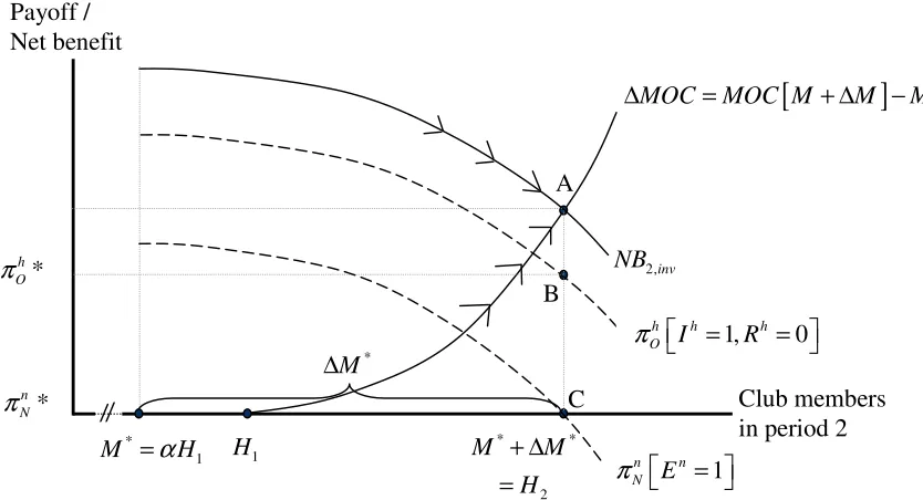
∆ is illustrated in Figure 2.

The figure depicts the adjustment process to the equilibrium (solid lines with arrows) and the

effect of an inflow of newcomers in period 2 on the payoffs of initial investors and

newcomers (dashed lines) in a setting with high transaction costs and intermediate elasticity

of new housing supply. Each additional newcomer to the neighborhood dilutes

[

]

2,new

NB M + ∆M . At the same time, MOC H

[ ]

increases with each additional housing unit built (the steepness of the curve is determined by the land scarcity H L in the neighborhood). Equilibrium is achieved when NB_2,new

[

M + ∆M

]

exactly equals the club good

marginal developer (point A). Note in this context that in stage 2 all residents will also be club

members, that is, H₂ =M+ ∆M and hence MOC H

[ ]

₂ =MOC M

[

+ ∆M

]

. In equilibrium, the marginal newcomer’s payoff from cooperating is exactly zero (point C), while the total

[image:18.595.79.496.192.418.2]

payoff of all investing homeowners (amount BC) is still positive.

Figure 2: Adjustment Process to Equilibrium and Equilibrium Payoffs

* * 2 M M H + ∆ = Club members in period 2

[

]

[ ]

1

MOC MOC M M MOC H

∆ = + ∆ − * n N π * h O

π NB2,inv

* M ∆ C B A Payoff / Net benefit 1 n n N E

π _{ =} _

1, 0

h h h

O I R

π _{ = =} _

1

H

* 1

M =αH

The membership levels in stage 1 and stage 2 are indeed stable equilibrium outcomes

because (i) they ensure a non-negative payoff for all club members and (ii) no member has an

incentive to deviate from the equilibrium. More generally, as long as the investment

conditions formulated in equations (11.1) and (11.2) hold, the equilibrium membership level

*

M in stage 1 and the change in the membership level *

M

∆ in stage 2 can be formulated as: *

1

M =αH (13.1)

(

)

* *

1

1- _new

M α H M H L

∆ = + _{ }, (13.2)

where

(

1-

α

)

H₁ denotes the empty (renter-occupied) housing units at the end of stage 1 that

need to be re-occupied by newcomers in stage 2 and where *

new

M _H L_ denotes the additional newcomers in stage 2 that occupy new housing units.

The homeownership rate

α

influences the initial investor’s equilibrium payoff in two

ways: An increase in

α

raises M* and thereby first increases then decreases the investor’s total payoff. At the same time, an increase in

α

reduces the number of renters exiting

voluntarily at the end of stage 1, reducing the inflow of newcomers *

M

2.3 Alternative Theoretical Frameworks and Derived Predictions

In the model presented above, relocation is endogenously determined and homeowners

and renters differ only in that relocation of a renter does not involve property transaction

costs. Adding a mobility shock to the model adds complexity but does not alter the main

predictions in significant ways. In a world with voluntary relocation and mobility shocks, the investment/free-riding decision is not only determined by transaction costs but also by the

likelihood that a homeowner receives a shock (i.e., free-riding is more likely if the probability

of a shock is high). Similarly, a homeowner’s payoff from investing in neighborhood specific

social capital is less likely to be positive if the probability of a mobility shock is high.

DiPasquale and Glaeser (1999) provide a formal analysis of the effects of mobility

shocks on social capital investment decisions. In their model mobility is induced by shocks,

whereas homeowners have a lower propensity than renters to receive a shock. Consequently,

homeowners have greater incentives to be ‘better citizens’. It is worth noting that DiPasquale

and Glaeser’s (1999) model and the one presented above also differ in the mechanisms

through which individual social capital investments lead to improved neighborhood quality.

In DiPasquale and Glaeser’s framework social capital ‘improves the ability of neighbors to

enjoy each other’s investments in local amenities’. In the model presented here, social capital

facilitates the production of utility generating club goods and individual social capital

contribution guarantees access to the club good related benefits. The two models differ in

another important aspect, DiPasquale and Glaeser do not model housing supply conditions.

As a consequence the model presented here makes additional (more refined) predictions with

respect to homeowners’ and renters’ decisions whether to invest in social capital. Specifically,

modeling housing market conditions generates Propositions 2 and 3, which are tested below.

3 Empirical Analysis

3.1 The Data

The data is derived from five main sources. The first source is the Restricted Use Data

version of the Social Capital Community Benchmark Survey (SCCBS) undertaken by the

Saguaro Seminar at the John F. Kennedy School of Government, Harvard University between

July 2000 and February 2001.19 As the survey title implies, this is the first attempt at

19

widespread systematic measurement of social capital, particularly within communities. The

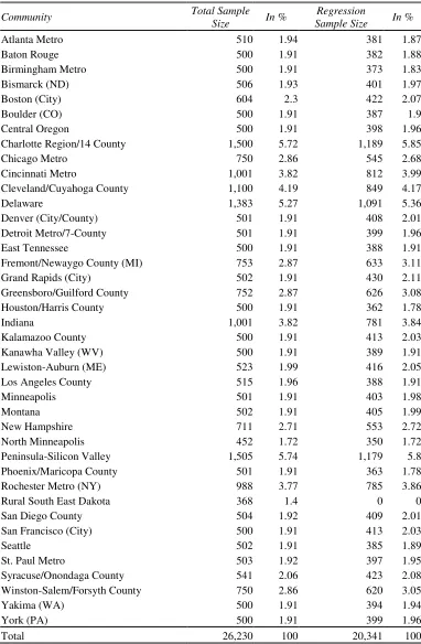
survey measures various manifestations of social capital as well as its suspected correlates in

41 U.S. ‘communities’ (a metro area, a city, or one or several counties). The ‘communities’

are listed in Appendix Table A1. The Restricted Use (in contrast to the Public Use) Data

version of the SCCBS provides geographical information including Census tract identifiers

for the survey respondents. The Census tract identifiers are subsequently used to merge the

SCCBS data with data from the other four main sources: the National Land Cover Data 1992

(NLCD 92), the Natural Amenity Scale Data (NASD), the NBER data repository, and the

2000 U.S. Census. Because the SCCBS Census tract information is based on 1990 boundary

definitions, all data is geographically matched to 1990 boundaries.

The NLCD 92 reports raster data including 21 different land uses with a spatial resolution

of 30 meters for 49 U.S. states. The Wharton GIS Lab geographically matched the raster data

to the Census tract level. This tract level land use data set can be used to derive the preferred

proxy measure for the inelasticity of new housing supply in a neighborhood: the share of

developed land in a Census tract. (A Census block group may be a better approximation of a

neighborhood in less urbanized areas. Unfortunately block level data is not consistently

available. However, it seems reasonable to assume that the land availability in a Census block

group and the corresponding tract are highly correlated.) The measure is defined as:

%-Developed =Developed land (residential, commercial, industrial, transport)

Developable land (all land except water, ice, barren, wetlands). (14)

The NASD provides detailed topography data at the U.S. county level. The data is

derived from the Economic Research Service, United States Department of Agriculture and is

used in the empirical analysis below to instrument for the share of developed land in a Census

tract. Similarly, the NBER data repository provides data on state level mortgage subsidy rates,

which are used as an instrument to identify a survey respondent’s homeownership status.20

Finally, the U.S. Census 2000 provides additional Census tract level controls including

the homeownership rate and the linguistic and ethnic heterogeneity.21 Alesina and LaFerrara

(2000) show that the latter two variables affect measures of social capital.

While the total SCCBS communities-sample consists of 26,230 adults, the regression

samples are somewhat smaller due to missing values.22 Most importantly, for some Census

20

The NBER provides a program (TAXSIM) that calculates federal and state income tax liabilities from survey data. As a ‘side product’ the NBER reports state-level income tax rates and corresponding mortgage subsidy rates. The URL is http://www.nber.org/~taxsim/state-rates (last accessed on July 24, 2007).

21

tracts that belong to the forty-one communities sample no corresponding land use data could

be matched. The final regression data set consists of four measures of individual social capital

investment and numerous household and location specific variables. All variables are

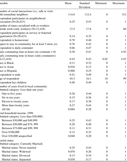
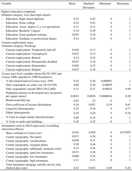
described in Section 3.3 below. Summary statistics are provided in Table 1.

3.2 Land Availability and the Elasticity of New Housing Supply

The empirical work that follows uses the share of developed land in a Census tract as a

proxy measure for the local inelasticity of new housing supply. The choice of this proxy measure is theoretically and empirically motivated. To begin with, the sheer impossibility of

converting land in built-up neighborhoods explains why highly developed locations have a

more inelastic supply of new housing compared to locations with plenty of open space.

The second argument is a purely mechanical one; mathematically, as long as the supply

curve has a positive price intercept, even a linear supply curve generates a positive

relationship between land scarcity and the supply inelasticity. A positive price intercept merely implies that the present value of future land rents from farming is greater than zero.

The third line of reasoning is founded in the endogenous zoning literature, which

considers land use restrictions as political outcomes determined by voting and lobbying.

While owners of developed land have an incentive to limit new housing supply to protect the

value of their assets, owners of undeveloped land have an interest in keeping land use

regulation flexible. Hence, to the extent that land use controls are the outcome of a political

process, new housing supply should be more inelastic in more developed locations where

owners of developed land (homeowners and landlords) are more numerous and politically

influential that owners of undeveloped land (e.g., farmers). Consistent with this reasoning,

Hilber and Robert-Nicoud (2006) provide empirical evidence that land scarcity has a causal

positive effect on the local regulatory restrictiveness. Various other studies provide support

for this finding. For example, Rudel (1989) demonstrates that municipalities in Connecticut

adopted land use laws later if they (i) are at a greater distance to New York City and (ii) had a

greater share of farmland. Moreover, increases in restrictiveness occurred in those places that

experienced the largest declines in farming during the 1960s. In a similar vein, Fischel (2004)

documents that land use regulation typically originates in the centers of large cities and then

spreads to the surrounding suburbs and towns. Finally, Glaeser, Gyourko and Saks (2005)

find a very high ‘regulatory tax’ for Manhattan condominiums but much lower values for the

22

entire metro area. Overall, these studies overwhelmingly support the view that undeveloped

land can be more easily converted into housing in less regulated locations at the edge of cities

but that conversion is costly and involves large time lags in more developed locations.

The final argument is based on the real options literature, which assumes that land

redevelopment is costly and developable open land therefore has an option value (Titman,

1985; Capozza and Helsley, 1990; Capozza and Li, 1994; Novy-Marx, 2005). In such a

setting, when a neighborhood becomes built-up, the incremental opportunity cost of building

an additional housing unit increases exponentially, implying inelastic supply of new housing.

While the evidence discussed above is circumstantial, Hilber and Mayer (2004) estimate

a structural model, using a well-identified strategy, to directly estimate supply elasticities for

locations with more and less developable land for future construction. Their findings suggest

that more developed communities indeed have more inelastic supply of new housing and a

greater extent of house price capitalization of local public school spending and local

amenities. In a related study, Brasington (2002) demonstrates, by splitting a sample into

houses on the interior and the edge of the urban area, that capitalization is weaker towards the

edge where housing supply elasticities and developer activity are greater. In a similar vein,

McDonald and McMillen (2000) show for Suburban Chicago that residential development is

greater in areas with a large proportion of agricultural land.

3.3 Empirical Specifications, Choice of Estimators and Identification Strategy

The base specification (Specification 1) estimates the effect of a survey respondent’s homeownership status (i.e., whether he or she owns) on particular measures of individual

social capital investments. Two of the measures are neighborhood specific (social

interactions with immediate neighbors23 and participation in neighborhood associations) and

two are non-neighborhood specific (social interactions with co-workers outside work and

participation in service and fraternal organizations). Specification 1 can be expressed as:

(

)

(

)

(

)

0 1 2

1

% .

K k+2 k

Individual contribution to social capital =

own developed control k

β β

β

β

ε

=

+ + +

∑

+ (15)

The respondent’s homeownership status (own) – the variable of interest in the base specification – is 1 if the respondent is a homeowner and 0 if he or she is renting. All else

23

equal, individual homeownership should be positively related to neighborhood specific social capital (

β

₁ >0) (Proposition 1) but unrelated or – because of substitution effects – possibly

negatively related to non-neighborhood specific social capital (

β

₁≤0) (Proposition 3). Besides the share developed land (%developed), the base specification includes a large number of location and household specific controls. The full set of controls is listed in Table

1. Previous research either predicts or has demonstrated that these variables are related to

various forms of social capital. The list of location specific controls includes a number of Census tract specific variables plus community sample fixed effects (one dummy variable for

each of the SCCBS-communities in the sample) to control for community specific

time-invariant unobservable characteristics. The Census tract specific controls are the homeownership rate, the income Gini coefficient, the linguistic heterogeneity, the ethnic

heterogeneity, the share of housing units in multi-unit buildings, the share of housing units in

single family detached homes and the population density in the developed area. The latter

variable is included as a proxy for the average proximity of residents. High residential

proximity may facilitate social interactions among neighbors because of shorter distances; on

the other hand, it may also create an environment of anonymity making social interactions

among immediate neighbors less likely, especially in multi-unit building environments.

The list of survey respondent specific controls includes the following variables: the number of years lived in the local community, whether the respondent expects to stay in the

community for at least 5 more years24, commuter characteristics, the race, the gender, the age

and age squared25, whether the respondent has children, household income category

dummies, the marital status, dummies for the highest education completed and dummies for

the current employment status. The effects of all these control variables on the different

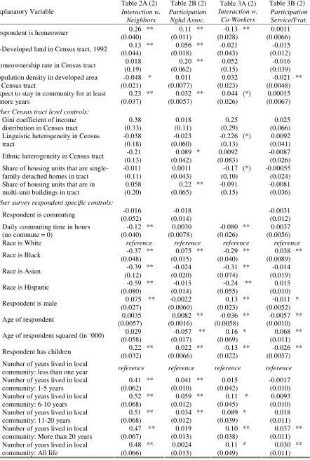
measures of individual social capital investment are reported in Appendix Table A2. Because

the coefficients and statistical significance levels of the control variables are overall similar

across all specifications, results are reported for the base specification only.

Specification 2 differs from the base specification in that it additionally includes the interaction effect between the survey respondent’s homeownership status (own) and the share of developed land in the tract (%developed):

24

Households are expected to engage more in social interactions if they plan to stay longer in their neighborhood or at their work place, suggesting a positive sign of the variable’s coefficient.

25

(

)

(

)

(

)

(

)

0 1 2

3

1

%

% .

K k+3 k

Individual contribution to social capital = own developed own developed control k

β β β

β β ε

=

+ + +

× +

∑

+ (16)

Theory predicts that individual homeownership should be more strongly positively

related to contributions to neighborhood specific forms of social capital in more developed places (

β

₃ >0), where such contributions have a stronger positive effect on property values

(Proposition 2). Again, theory makes a different prediction for contributions to

non-neighborhood specific forms of social capital; the respondent’s homeownership status and the

interaction effect ‘homeownership× developed’ should not be positively linked to

non-neighborhood specific forms of social capital (

β

₃≤0; Proposition 3).

The two specifications are first estimated using ordinary least squares (OLS).26 Next,

various endogeneity concerns are addressed by applying a two-stage-least-squares (2SLS)

estimator. The first potential endogeneity concern is related to the land scarcity variable; neighborhoods with more active homeowners may enact more restrictive zoning laws and

other regulations that limit housing supply. Similarly, one could make a case that the

population density variable is endogenously determined; restrictive zoning laws may affect the population density in the developed area of the neighborhood for example via minimum

lot size restrictions. The endogeneity concern related to the land scarcity variable is

somewhat alleviated by the fact that the land use data was collected in 1992, while all other

variables including the homeownership status of the survey respondents and the social capital

measures are from the year 2000. Social capital investments in 2000 should not explain the

share of developed land 8 years earlier. Secondly, if more active homewners enact stricter

zoning that preserves open land then one should find that the coefficient of the interaction

term ‘own×developed’ has a negative sign. However, as is demonstrated below, the opposite

is the case. Thus, the bias goes against the predicted results.27 Nevertheless in order to fully

address the endogeneity concerns related to the land scarcity and the population density

variables, instrumental variable estimates were carried out. As instruments for land scarcity

26

The probability of participation in neighborhood or service/fraternal organizations could also be estimated using logit or probit models. However, a linear probability model is preferred because the interpretation of interaction effects in logit and probit models is not straightforward. This is because the magnitude of an interaction effect in a non-linear model does not equal the marginal effect of the interaction term and can be of opposite sign. Standard statistical software does not calculate the correct standard errors (Ai and Norton, 2003).

27

and population density in the developed area, physical limits on the housing supply in the

Census tract are used. The list of instrumental variables includes the share of wetland in the

Census tract and a number of county specific dummy variables for different topography types

(flat plains, smooth plains, irregular plains, tablelands and moderate relief, open low

mountains, low mountains and high mountains). These features of the Census tracts are

expected to explain the share of developed land and the population density within the

developed area but should be unrelated to the error term. As Wooldridge (2002)

demonstrates, the product of an instrument for a given endogenous variable and an

exogenous component of an interaction term is also a valid instrument. Consequently, the

interaction term ‘own × developed’ is identified using the following instruments: the

respondent’s homeownership status interacted with the share wetland in the Census tract plus

the homeownership status variable interacted with each of the 7 topography type dummies.

Another potential endogeneity concern is related to the survey respondent’s

homeownership status. Omitted variables that may explain the respondent’s homeownership status may also be correlated to the four measures of social capital. In order to address this

potential issue – and provide a further robustness check – additional instrumental variables

are used to identify the respondent’s homeownership status and the variable’s interaction

with land scarcity. The identification strategy exploits two facts: (i) that homeowners in the

United States can deduct mortgage interest from their income taxes and (ii) that this tax

subsidy differs across U.S. states.28 Rather than using each survey respondent’s specific

subsidy rate, the total maximum mortgage subsidy rate by state is used. This variable

measures the state-specific maximum total subsidy related to both federal and state income

tax. The measure has the advantage that it is independent of individual decisions as well as of

the within state income distribution. The total maxim subsidy rate should explain a survey

respondent’s homeownership propensity but should not be a function of individual social

capital contributions. More precisely, the maximum subsidy rate should have a differential

impact on a respondent’s homeownership propensity depending on his or her income (i.e.,

mortgage rate subsidies benefit higher incomes much more than lower incomes). Hence, the

total maximum mortgage subsidy rate by state interacted with each income category dummy

is used as an instrument to identify the homeownership status of the survey respondent.

Again following Woolridge (2002), the instruments to identify the interaction term

28