Munich Personal RePEc Archive
Likelihood-based inference for correlated
diffusions
Kalogeropoulos, Konstantinos and Dellaportas, Petros and
Roberts, Gareth O.
University of Gambridge, Engineering Department - Signal
Processing Laboratory, Athens University of Economics and
Business, Statistics Department, University of Warwick, Statistics
Department
2007
Online at
https://mpra.ub.uni-muenchen.de/5696/
Likelihood based inference for correlated diffusions
Konstantinos Kalogeropoulos
∗University of Cambridge, Department of Engineering - Signal Processing Laboratory
Petros Dellaportas
Athens University of Economics and Business, Department of Statistics
Gareth O. Roberts
University of Warwick, Department of Statistics
October 22, 2007
Abstract
We address the problem of likelihood based inference for correlated diffusion processes using
Markov chain Monte Carlo (MCMC) techniques. Such a task presents two interesting problems.
First, the construction of the MCMC scheme should ensure that the correlation coefficients are
updated subject to the positive definite constraints of the diffusion matrix. Second, a diffusion
may only be observed at a finite set of points and the marginal likelihood for the parameters
based on these observations is generally not available. We overcome the first issue by using
the Cholesky factorisation on the diffusion matrix. To deal with the likelihood unavailability, we
generalise the data augmentation framework of Roberts and Stramer (2001 Biometrika
88(3):603-621) tod−dimensional correlated diffusions including multivariate stochastic volatility models.
Our methodology is illustrated through simulation based experiments and with daily EUR /USD,
GBP/USD rates together with their implied volatilities.
Keywords: Markov chain Monte Carlo, Multivariate stochastic volatility, Multivariate CIR model, Cholesky Factorisation.
1
Introduction
Diffusion processes provide a natural model for phenomena evolving continuously in time. One of
their appealing features is that they are defined in terms of the instantaneous mean and variance
of the process. Specifically, a diffusionxtobeys the dynamics of the following stochastic differential
equation (SDE)
dxt=µ(t, xt, θ)dt+σ(t, xt, θ)dwt, (1)
driven by standard Brownian motion wt. The functions µ(.) and σ(.) are termed as the drift and
the volatility of the diffusion respectively. Throughout this paper we suppress the dependence on t
to simplify the notation, but the methodology is also applicable to time inhomogeneous diffusions.
The diffusion process xtis well defined if (1) has a unique weak solution, which translates into some
regularity conditions (locally Lipschitz with a linear growth bound) onµ(.) andσ(.); see chapter 5 of
Rogers and Williams (1994) for more details.
We address the problem of modelling several diffusions, denoted by x{ti}, i = 1, . . . , d. Each
diffusion x{ti} may have a drift µ{i}(.) and volatility σ{i}(.) of general, yet known, form. We also
allow for correlations,corr(dx{ti}, dx
{j}
t )=ρij =ρji,i6=j, on the instantaneous increments. The use
of cross-correlations is quite common when modelling multivariate time series, as they may capture
effects caused by common factors of the underlying stochastic processes. In this paper we illustrate
our methodology through two examples of correlated diffusions. The first example targets interest
rates and bond pricing. Such time series often exhibit strong inter-dependencies; for instance, interest
rates may correspond to similar bonds but with different expiry dates, thus giving rise to correlations
among them. In Section 5 we examine a multivariate version of the Cox et al. (1985) model (CIR),
often used for such data. The second example considers currency pairs which are known to be
correlated, possibly due to the common currencies they may represent. Section 6 contains an analysis
on EUR/USD and GBP/USD data, based on multivariate versions of stochastic volatility diffusions,
such as the model of Heston (1993). In both examples, the inclusion of correlations in the model is
essential for two reasons. First, they may affect the parameter estimates of the individual diffusions,
the bond/option pricing procedure.
We proceed by combining the diffusionsx{ti} together intoXt= (x{t1}, . . . , x
{d}
t )′ (with′ denoting
transposition), so that Xt is ad−dimensional vector for each time t. The diffusion matrix ofXt,A,
denotes its instantaneous covariance and takes the following form:
A:=
σ{1}(.)2 ρ
12σ{1}(.)σ{2}(.) . . . ρ1dσ{1}(.)σ{d}(.)
ρ12σ{1}(.)σ{2}(.) σ{2}(.)2 . . . ρ2dσ{2}(.)σ{d}(.)
..
. ... . .. ...
ρd1σ{1}(.)σ{d}(.) ρd2σ{2}(.)σ{d}(.) . . . σ{d}(.)2
(2)
The diffusion processXtis defined through the following multi-dimensional SDE
dXt=M(Xt, θ)dt+ Σ(Xt, θ)dWt, (3)
where Wt is a d−dimensional Brownian motion with independent components, with vector valued
driftM : [0,+∞)× SX×Θ→ ℜd with [M(.)]i =µ{i}(.), and matrix valued volatility (also termed
as dispersion matrix) Σ(·) : [0,+∞)× SX×Θ→ ℜd×d, whereSX and Θ denotes the domain of the
diffusionXtand the parameter vectorθrespectively. The dispersion matrix Σ is a square root of the
instantaneous covariance matrix A = ΣΣ′. To ensure a unique weak solution for X
t, we require a
unique weak solution for eachx{ti} and the matrix Ato be positive definite for allt, Xt, θ.
Each diffusion x{ti} may be observed, with or without error, at a finite set of points, or may be
entirely unobserved. The diffusion will be termed as directly observed in cases with exact
obser-vations on all x{ti}, and partially observed otherwise. For ease of exposition, the methodology of
this paper is initially presented for directly observed diffusions, and adaptations to partial
obser-vation regimes, as in multivariate stochastic volatility models, are provided when necessary.
Sim-ilarly, we consider observations of the entire vector of Xt at each time, although this assumption
can easily be relaxed. We denote the times of observations by tk, k = 1, . . . , n, and the data with
Y =nYk=Xtk = (x
{1}
tk , . . . , x
{d}
tk )
′, k= 1, . . . , no. Our aim is to draw likelihood based inference for
the parameter vectorθ given these observations.
The task of inference on diffusions observed discretely in time is generally not trivial and has
The main problem is that the likelihood is generally not available except for a few cases. This has
stimulated various techniques based on likelihood approximations. Approximations may be analytical
(A¨ıt-Sahalia, 2005), or simulation based; see Pedersen (1995) or a refinement of this technique Durham
and Gallant (2002). They usually approximate the likelihood in a way so that the discretisation error
can become arbitrarily small, although the methodology developed in Beskos et al. (2006a) succeeds
exact inference in the sense that it allows only for Monte Carlo error.
We shall adopt a Bayesian approach using Markov chain Monte Carlo (MCMC) method. Since
diffusions are not completely observed, it is natural to use data augmentation (Tanner and Wong,
1987), treating the segments of diffusion sample path (or a suitably fine approximation to this) as
missing data. Initial MCMC schemes of this type were introduced by Jones (1999), Eraker (2001)
and Elerian et al. (2001). However, as noted in the simulation based experiment of Elerian et al.
(2001), and established theoretically by Roberts and Stramer (2001), the algorithms introduced in
these initial implementations of MCMC in this context degenerate as the number of imputed points
increases. The problem may be overcome for scalar diffusions with the reparametrisation of Roberts
and Stramer (2001). An alternative reparametrisation is provided by Golightly and Wilkinson (2007),
see also Golightly and Wilkinson (2006) for a sequential approach, which can in principle be applied
in principle to any diffusion.
However, the adaptation of such MCMC scheme to multivariate diffusions introduces additional
issues. The task of updating the covariance matrix A is generally not trivial, as its full conditional
posterior is most of the times intractable, and the use of Metropolis steps is inevitable. It is therefore
crucial, especially for high-dimensional diffusions, to update the covariance matrix componentwise as
the discrepancy between proposed and current moves is increasing ind. This introduces the problem
of preserving the positive definite structure of the diffusion matrix A. Note that drawing samples
from the posterior of covariance matrices, which may not necessarily be diffusion matrices, is a general
MCMC issue and usually requires appropriate matrix decompositions; see for example Pinheiro and
Bates (1996) and Daniels and Kass (1999).
The contribution of this paper is two-fold. First, we introduce a natural and general framework
factorisation ofAand enables us to define Σ explicitly. The MCMC algorithm may then be
appropri-ately designed to provide samples from the posterior of Σ, which can be transformed toAat any time
through the Cholesky decomposition. This framework may be coupled with any of the previously
mentioned likelihood approximation techniques, such as those of Beskos et al. (2006a) or A¨ıt-Sahalia
(2005), to perform Bayesian inference for the parameters of the multi-dimensional diffusion. Second,
we offer a full and stand alone MCMC scheme which combines the Cholesky decomposition with the
reparametrised data augmentation approach of Roberts and Stramer (2001). This scheme may be
used for parameter estimation of several multivariate diffusion models including stochastic volatility.
The use of data augmentation is justified by its convenient property to be applicable at both directly
and partially observed diffusions.
The paper is organised as follows: Section 2 describes the structure of a data augmentation scheme
and highlights potential problems regarding the irreducibility of the MCMC algorithm. These
prob-lems may be tackled with the reparametrisation of this paper which requires the Cholesky factorisation
of the diffusion matrix, presented in Section 3. Specific MCMC implementation details are given in
Section 4 and the methodology of this paper is illustrated through simulated data in Section 5, and on
daily EUR/USD, GBP/USD currency pairs in Section 6. Finally, we summarise in Section 7 adding
some discussion and links to some other relevant work.
2
Data augmentation and degeneracy issues
2.1
The problem in practice
Data augmentation scheme bypasses the problem of simulating directly from the posterior π(θ|Y),
which is typically unavailable for discretely observed data. The idea is to introduce a latent variable
X that simplifies the likelihoodL(Y;X, θ). We use the following two steps:
1. Simulate X conditional on Y and θ.
2. Simulate θ from the augmented conditional posterior which is proportional to
Our problem can easily be adapted to this setting. Y represents the observations of the price
process Xt, and X contains discrete skeletons of the diffusion paths between Y. Thus, X and Y
constitute the augmented dataset Xiδ, i = 0, . . . , T /δ, which is a fine partition of the multivariate
diffusion Xt withδ controlling the amount of augmentation. Based on this partition the likelihood
can be approximated, for example via the Euler-Maruyama approximation
LE(Y;X, θ) =
T /δ
Y
i=1
p(Xiδ|X(i−1)δ),
Xiδ|X(i−1)δ ∼ N X(i−1)δ+δM(X(i−1)δ, θ), δA(X(i−1)δ, θ)
, (4)
which is known to converge to the true likelihood L(Y;X, θ) for smallδ(Pedersen, 1995).
Another property of diffusions relatesA(Xt, θ) with the quadratic variation process. Specifically
it is well-known that
lim
δ→0
T /δ
X
i=1
Xiδ−X(i−1)δ
Xiδ−X(i−1)δ
′
=
Z T
0
A(Xs, θ)ds a.s. (5)
The solution of the equation above determines the diffusion matrix parameters exactly. Hence, there
exists perfect correlation between these parameters andXasδ→0. Thus for the theoretical algorithm
which imputes the entire X path, the MCMC algorithm is reducible. In practice this means that
as the proportion of imputed data points increases mixing problems for the MCMC chain become
progressively worse This phenomenon was first noted in Roberts and Stramer (2001) and Elerian
et al. (2001). As would be expected, the EM algorithm suffers from the same problem.
2.2
Measure theoretic probability viewpoint
In this section, we explore the problem from a different angle, through a slightly more rigorous look at
the likelihood. LetXtbe a diffusion that satisfies (3) and assumeX0=Y0andX1=Y1,Y = (Y1, Y2).
Denote the probability law ofX byPθ and that of its driftless version,
dMt=σ(Xt, θ)dWt,
by Qθ. To write down the likelihood, we can use the Cameron-Martin-Girsanov formula which
dPθ
dQθ
= G(X, M, A) = exp
( Z T
0
A(Xs, θ)−1M(Xs, θ)
′ dXs
−12
Z T
0
M(Xs, θ)′A(Xs, θ)−1M(Xs, θ)ds
)
.
Note that the expression above contains stochastic and path integrals for which an analytic solution
is generally not available. However, given a sufficiently fine partition of the diffusion path, they can
be evaluated numerically providing an approximation of the likelihood which is equivalent to (4).
Now assume for a moment that underQθthe marginal density ofY with respect tod−dimensional
Lebesgue measure Lebd(Y), is known and denote byfM(Y;θ). The dominating measure Qθ can be
factorised in the following way
Qθ=QYθ ×Lebd(Y)×fM(Y;θ), (6)
where QYθ is the measureQθ conditioned on the observationsY. We can now write
dPθ
QY
θ ×Lebd(Y)
(Xmis, Y) = G(X, M, A)×fM(Y;θ). (7)
The expression in (7) provides the likelihood for the latent diffusion pathsXmisand the parameters
θ. However, this likelihood is not valid because its reference measure, Qyθ, depends on parameters.
Furthermore, since the volatility parameters are identified by the quadratic covariation process, the
measureQθis just a point mass. Consequently, the measuresQθare mutually singular and therefore
so are Pθ. Hence, inference for both Xmis, θ is not possible using a common σ−finite dominating
measure. In the next section, we specify an appropriate transformation of the diffusion that allows
a likelihood specification with respect to a parameter-free dominating measure. This transformation
may be viewed as a generalisation of the one in Roberts and Stramer (2001). The transformed
diffusion has unit volatility, thus the problems induced by the quadratic variation property of (5) are
3
Likelihood specification
3.1
A Cholesky factorisation of the diffusion matrix
Consider the multi-dimensional SDE of (3) with the diffusion matrixAof (2). Thed×dmatricesAand
Σ are linked throughA= ΣΣ′, therefore Σ is not unique. However, it is crucial to define Σ explicitly
and establish a 1-1 mapping withA, as each one of these two matrices may be more convenient for
different reasons. The likelihood, defined either through the Euler-Maruyama approximation in (4) or
through Cameron-Martin-Girsanov’s formula in (7), is expressed in terms ofA, which is also the main
target of inference. On the other hand Ais a positive definite matrix, whereas the only assumption
made on Σ requires its full rank. Hence it is generally more convenient to work with Σ in the context
of a MCMC algorithm. Moreover, as mentioned in the previous section, the generalisation of the
Roberts and Stramer (2001) reparametrisation involves a transformation to unit volatility which will
naturally be based on Σ.
In this paper, we define Σ using the Cholesky decomposition ofA. LetSx(Xt, θ) =diag{σ{i}(Xt, θ)}.
The diffusion matrix may then be factorised in the following way
A(Xt, θ) = Sx(Xt, θ)R Sx(Xt, θ),
where R is the correlation matrix. One may define Σ as the product of Sx with the Cholesky
decomposition of R, say C. But the elements of C will not have the general Cholesky structure, since
R has the additional property of being a correlation matrix. To eliminate such problems we write
eachσi(Xt, θ) as
σ{i}(X
t, θ) =cif{i}(Xt, θ), ∀i, (8)
for some positive constants ci. This imposes no restrictions as we can always set f{i}(Xt, θ) =
σ{i}(X
t, θ)/ci, see Section 3.4 for such an example. Now, based onFx(Xt, θ) =diag{f{i}(Xt, θ)}, we
can use (8) to obtain an alternative decomposition ofA,
where V is a general symmetric positive definite matrix with
Vij =
c2
i, i=j
ρijcicj, i6=j.
(9)
The Cholesky decomposition of V, denoted by C (V = CC′), may now be used. The dispersion
matrix Σ(Xt, θ) is defined as
Σ(Xt, θ) = Fx(Xt, θ)C. (10)
In coordinate form, Σ may be written as
[Σ(Xt, θ)]ij=
[C]ijfi(Xt, θ), j≤i
0, j > i.
The only restriction on the constants Cij requires compatibility with the Cholesky decomposition,
which translates on positive diagonal entriesCii. As we mention in 4.2, this is particularly convenient
in a MCMC environment and specifically for componentwise updates of Σ(Xt, θ) parameters. The
Cholesky decomposition establishes the 1-1 mapping between Σ and A and ensures that the entire
space of diffusion matrices as Ais covered.
3.2
Transformation to unit volatility
In Section 2, the need for a reparametrisation was highlighted in order to avoid degenerate MCMC
algorithms. Roberts and Stramer (2001) provide a solution to the problem for scalar diffusions,
which involves a transformation to unit volatility. However, in more than one dimensions such a
transformation does not always exist, as noted A¨ıt-Sahalia (2005). When such a transformation is
available the diffusion is said to be reducible, a term introduced by A¨ıt-Sahalia (2005) who also
provides a necessary and sufficient condition for reducibility: diffusions with non-singular Σ(Xt, θ)
are reducible if and only if
∂[Σ(Xt, θ)−1]ij
∂x{tk}
= ∂[Σ(Xt, θ) −1]
ik
∂x{tj}
, ∀i, j, k∈ {1, . . . , d}, withj < k (11)
Not all SDEs with diffusion matrixAas in (2) or dispersion matrix Σ as in (10) are reducible. In
this section, we restrict our attention to diffusions with
σ{i}(X
for which we prove the reducibility. This is established by the following proposition:
Proposition 3.1 Let X be ad-dimensional diffusion which obeys the following SDE:
dXt=M(t, Xt, θ)dt+ Σ(t, Xt, θ)dWt.
Furthermore, assume that
Σ(Xt, θ) = Fx(Xt, θ)C,
where Fx(Xt, θ) =diag{f{i}(x{ti}, θ)} and C is a lower triangular matrix with positive diagonal
ele-ments. The diffusion X can then be transformed to one with identity diffusion matrix. In other words
X is reducible.
Proof: See Appendix.
The next proposition provides explicitly a transformation to unit volatility. It may be viewed as an
alternative proof of proposition 3.1
Proposition 3.2 Consider the setting and the diffusion Xt of proposition 3.1. Suppose that there
exist g{i}(x
t{i}, θ)fori= 1, . . . , d with continuous second derivatives, so that
∂g{i}(x{i}
t , θ)
∂x{ti}
= 1
f{i}(x{i}
t , θ)
, j= 1, . . . , d,
and letGx(Xt, θ) =
g{1}x{1}
t , θ), . . . , g{d}(x
{d}
t , θ)
′
. Consider the transformation
H(Xt, θ) =
h{1}(Xt, θ), . . . , h{d}(Xt, θ)
′
=C−1Gx(Xt, θ). (13)
The diffusionUt=H(Xt, θ)has then unit volatility.
Proof: See Appendix.
The transformation of (13) may be used to specify the likelihood under an appropriate
reparametri-sation which will ensure a non - decreasing efficiency, of the data augmentation MCMC scheme, in the
level of augmentation. Notice that the transformation of (13) to unit volatility is not unique. This is
not necessary for our methodology, in fact we only require its invertibility which is ensured as long as
eachgi(xt{i}, θ) is itself invertible. We present this reparametrisation in the Section 3.3, whereas in
3.3
Reparametrised likelihood
Consider the diffusion that satisfies the SDE of (3) where the driftM(.) and Σ satisfy the appropriate
conditions so that Xt has a unique weak solution and Ito’s lemma can be applied. Furthermore,
assume that
Σ(Xt, θ) = Fx(Xt, θ)C,
where Fx(Xt, θ) =diag{f{i}(x{ti}, θ)} and C is a lower triangular matrix with positive diagonal
ele-ments. For ease of illustration let the entire vector ofXtbe observed at each time and denote the times
of observations bytk, k= 0, . . . , n, and the data withY =
n
Yk =Xtk= (x
{1}
tk , . . . , x
{d}
tk )
′, k= 1, . . . , no.
We will define the likelihood for a pair of successive observations, (Yk−1, Yk). Due to the Markov
property of diffusions, the full likelihood is just given by the product of all pairs of consecutive
obser-vations. Without applying a reparametrisation, the likelihood can be defined through (7). However,
as discussed in 2, this likelihood is problematic because it is written with respect to a dominating
measure that depends on parameters. The aim of the reparametrisation is to obtain a likelihood with
a parameter-free dominating measure.
The first step of the reparametrisation requires a transformationUt=H(Xt, θ) = u{1}, . . . , u{d}
′ ,
so that the diffusion matrix ofUtis thed−dimensional identity matrix. As established by proposition
3.1, such a transformation does exist and can be obtained explicitly by (13). The SDE of the r−th
coordinate of the transformed diffusion U will be given by:
du{tr}=µ
{r}
U (Ut, θ)dt+dw
{r}
t , r= 1, . . . , d,
with
µ{Ur}(Ut, θ) = d
X
i=1
∂hr(Xt, θ)
∂x{i} µ {i}(X
t, θ) + d
X
i=1
∂2h
r(Xt, θ)
∂(x{i})2 [Σ(Xt, θ)] 2
ii,
where Xt may replaced with H−1(Ut, θ) so that the SDE is expressed in terms of Ut. If we use the
Cameron-Martin-Girsanov formula in a similar manner as in Section 2.2, we can write the likelihood
as
dPθ
WYH
×Lebd(YH)
Umis, Y
= G(U, µU, Id)fM(Y;θ),
or equivalently
dPθ
WYH
×Lebd(Y)
Umis, Y
where WYH
is just Wiener measure conditioned on the transformed observations YH=H(Y, θ),
N(Y, V) denotes the Gaussian density of Y under 0 mean and covariance V, and J(Y, θ) is the
Jacobian term from the transformationH(Y, θ). The dominating measure of the likelihood,WYH,
re-flects the distribution ofdindependent Brownian bridges withYHas endpoints and therefore depends
on parameters. For this reason we introduce a second transformation
z{i}(s) =u{i}(s)−(tk−s)H(y {i}
k−1, θ)(tk−1) + (s−tk−1)h(y{ki}, θ)
tk−tk−1
, tk−1< s < tk, (14)
for alli∈ {1, . . . , d}, which centers the bridge to start and finish at 0 and preserves the unit volatility.
LetZ= z{1}, . . . , z{d}′
and the functionU =η(Z) to be the inverse of 14. The SDE forZ becomes
dz{ti}=µ
{i}
Ut(η(Zt), θ)dt+dw
{i}
t , ∀i∈ {1, . . . , d}
The likelihood may now be written as
dPθ
W0)×Leb
d(Y)
Zmis, h(Y, θ)
= G(η(Zt), MU, Id)× N YkH−YkH−1, Id
|J(Y, θ)|, (15)
where
MU =
µ{U1t}(η(Zt), θ), . . . , µ
{d}
Ut (η(Zt), θ)
′
.
The dominating measure of the likelihood provided by 15 does not depend on any parameters, being
the product of d independent Brownian bridges that start and finish at 0. The likelihood of (15)
may be used to construct an irreducible MCMC scheme which will not degenerate as we increase the
amount of augmentation. The stochastic and path integrals involved cannot be solved analytically
but they can be evaluated numerically given a sufficiently fine partition of the diffusion path. Note
also that, as a result of these transformations, inference will now be based on Zt rather than Xt.
However, the posterior draws ofZt may be inverted to provide samples from the posterior ofXt.
3.4
Multivariate stochastic volatility models
In the previous subsection we assumed a diffusion with SDE that satisfies (12) so that the
trans-formation of (13) is directly applicable. However, there exist interesting diffusion models outside of
this class with a broad range of applications. One famous example of such models is provided by
models, including those of Hull and White (1987), Stein and Stein (1991) and Heston (1993), belong
to the following general class of 2−dimensional SDEs
dxt dvt =
µx(vt, θ)
µv(vt, θ)
dt+
σx(vt, θ) 0
0 σv(vt, θ)
dbt dwt , (16)
where bt and wt are correlated standard Brownian motions, xt usually denotes the log price, whose
volatility is provided by another diffusionvt.
Diffusions that satisfy SDEs as in (16) cannot generally be transformed to unit volatility
(A¨ıt-Sahalia, 2005), as the reparametrisation of 3.3 requires. Nevertheless, it is still possible to construct
an irreducible data augmentation scheme to estimate their parameters. As noted in Chib et al. (2005)
the conditional likelihood ofxt, givenvt, is available in closed form and therefore only the paths ofvt
need to be imputed to approximate the likelihood. Consequently, as shown in Kalogeropoulos (2007),
it suffices to transformvt itself to unit volatility.
This idea may be coupled with the Cholesky factorisation to handle multivariate stochastic
volatil-ity models. We illustrate this for the case of a bivariate Heston model. The scalar Heston model can
be written as
dxt =
µx−1
2v
2
t
dt+√vtdbt,
dvt = κ(µv−vt)dt+σ√vtdwt.
where btandwtare correlated. We can re-write the top equation, by settingc=õv, to
dxt=
µx−1
2v
2
t
dt+c
rv
t
µv
dBt.
Based on the formulation above, a bivariate Heston model may be written as a 4−dimensional diffusion
Xt=
vt{1}, v
{2}
t , x
{1}
t , x
{2}
t
′
, withx{t1}, x
{2}
t denoting the log-prices, andv
{1}
t , v
{2}
t their volatilities.
The diffusion matrix now has the general form of (2) all of the components ofXtmay be correlated.
dv{t1}
dv{t2}
dx{t1}
dx{t2}
= κ1
µ1−v{t1}
κ2
µ2−v{t2}
µ3−12(vt{1})2
µ4−12(vt{2})2
dt + Fx(Xt, θ)C dBt, (17)
where now Btis a 4−dimensional Brownian motion with independent components,
Fx(Xt, θ) =diag
q
vt{1},
q
vt{2},
q
v{t1}
µ1
,
q
vt{2}
µ2
,
andCis the lower triangular Cholesky matrix whose entriesCij may be seen as a 1-1 transformation
of parameter vector containing the correlationsρij, and alsoσ1,σ2,√µ1 and√µ2.
Regarding the likelihood, consider again a pair of successive observations, Yk−1, Yk with Yk =
(yk{3}, yk{4}), forx{t1}, x
{2}
t . Conditional onv
{1}
t , v
{2}
t , and therefore also on their corresponding
Brow-nian componentsb{t1}, b
{2}
t , the likelihood forYk is a bi-variate Gaussian with mean
y{k3−}1+Rtk
tk−1
µ3−12(v
{1}
s )2
ds+C31
Rtk
tk−1
q
vs{1}
µ1 db
{1}
s +C32
Rtk
tk−1
q
v{s1}
µ1 db
{2}
s
y{k4−}1+Rtk
tk−1
µ4−12(v{s2})2
ds+C41Rt
k
tk−1
q
vs{2}
µ2 db
{1}
s +C42Rt
k
tk−1
q
v{s2}
µ2 db
{2}
s ,
and covariance matrix
Rtk
tk−1C
2 33
v{1}
s
µ2 3 ds
Rtk
tk−1C33C43
√ v{1}s v
{2}
s
µ3µ4 ds
Rtk
tk−1C33C43
√ v{1}s v
{2}
s
µ3µ4 ds
Rtk
tk−1(C
2
43+C442)
v{2}s
µ2 4 ds .
The integrals above cannot be computed analytically, but the augmented path ofv{t1}, v
{2}
t enables
accurate numerical approximations of them.
The remaining part of the likelihood may be obtained through the reparametrisation recipe of
Section 3.3, modified according to the observation regime of the volatility. In some cases the
volatil-ity may be entirely unobserved, leading to a partially observed diffusion. Nevertheless alternative
formulations are available, where information from option prices is used to construct exact or noisy
volatility observations; see for example A¨ıt-Sahalia and Kimmel (2005), Chernov and Ghysels (2000)
and Kalogeropoulos et al. (2007). In the presence of exact observations the transformations of (13)
and (14) may be used. Note that transformation to unit volatility refers to the 2-dimensional diffusion
(vt{1}, v
{2}
t )′, rather than the entireXt. For the bivariate Heston model it takes the following form
where
Gx(Xt) =
2
q
x{t1},2
q
x{t2}
′
,
and D is a block of C containing theCij entries with i, j ={1,2}. If the observations are noisy or
they do not exist at all, the transformation of (14) may be replaced with
Z{i}(s) =U{i}(s)−U0, 0< s < tn,
and theN YH
k −YkH−1, Id|J(Y, θ)|part of the likelihood should be replaced with the relative noise
density or removed accordingly.
The above likelihood specification can be applied to all multivariate stochastic volatility models
that satisfy the SDE of 16. For more complex models, the framework of Golightly and Wilkinson
(2007) or time change transformations of Kalogeropoulos et al. (2007) may be combined with the
Cholesky factorisation.
4
MCMC implementation
Based on the likelihood specifications of the previous section, it is now possible to construct an
irreducible data augmentation MCMC scheme. The algorithm may be divided into three parts: the
updates of the diffusion paths Zmis, the parameters of the dispersion matrix Σ(X
t, θ) and those of
the drift M(Xt, θ). Generally, the updates of the drift parameters may be executed using standard
random walk Metropolis techniques, although for some diffusion models the full conditionals may be
analytically tractable and Gibbs steps may be used instead. Hence, in the next two subsections we
provide some details regarding the updates of the diffusion paths and the volatility parameters.
4.1
Updating the imputed paths
There exist several options for carrying out this step and most of them are based on an independence
sampler. For discretely observed diffusions the augmented path may be divided inton×ddiffusion
bridges connecting the observed points, and each one of them may be updated in turn. The full
conditional of Zmis may be written as
dPθ
dW0(Z
mis
|Y) =G(η(Zt), MU, Id)
fM(Y;A)
where fX(Y;A) is the density ofY with respect to the Lebesgue measure underPθ. Note that this
expression will be slightly different for stochastic volatility models.
The dominating measure of the likelihood W0, in other words a Brownian bridge, may be used
as the proposal distribution for the independence sampler. Based on (18), the algorithm will then
contain the following steps
• Step 1: Propose a Brownian bridge from tk−1 to tk.
• Step 2: Substitute into i-th dimension and form Z∗
t.
• Step 3: Accept with probability:
min
1,G(η(Z ∗
t), MU, Id)
G(η(Zt), MU, Id)
.
• Repeat for all k= 1, . . . n and i= 1, . . . , d.
The algorithm above takes advantage of the transformation to unit volatility and splits the path
into n×dindependent, under the dominating measure, bridges. Alternative proposals are available
such as the diffusion bridges introduced in Durham and Gallant (2002) and Delyon and Hu (2007),
which can be adapted in a MCMC setting through the reparametrisation framework of Golightly and
Wilkinson (2007). Another option is to propose local moves of the paths in the spirit of Beskos et al.
(2006b). This approach may be viewed as a random walk metropolis in the space of diffusion bridges.
Note however that this technique requires bridges with unit volatility, and therefore it can only be
used for correlated diffusions through the reparametrisation framework of this paper.
Further increase in the acceptance rate may be achieved by choosing a proposal distribution which
is closer to the targetPθ, for example a linear diffusion bridge. Suppose that we propose from another
diffusion bridge distribution, denoted byL0, with driftL. We can now write:
dPθ
dL0(Zmis|Y) =
dPθ/dW0
dL0/dW0
(Zmis|Y)∝G(η(Zt), MU, Id)
G(η(Zt), L, Id)
(19)
Based on (19), the corresponding algorithm, termed as method B in Roberts and Stramer (2001),
will consist of the following steps:
• Step 2: Substitute into i-th dimension and form Z∗
t.
• Step 3: Accept with probability:
min
1,G(η(Z ∗
t), MU, Id)G(η(Zt), L, Id)
G(η(Z∗
t), L, Id)G(η(Zt), MU, Id)
.
• Repeat for all k= 1, . . . n and i= 1, . . . , d.
However, low acceptance rates may still occur, especially in sparse datasets. In such cases, each
bridge may be further split into smaller blocks and updating strategies based on overlapping or random
sized blocks may be advocated; see Kalogeropoulos (2007) and Chib et al. (2005) for more details.
These techniques may also be used in partially observed diffusions, for example in stochastic volatility
models, where some components of the diffusion may be observed with error or not be observed at
all.
4.2
Updating the volatility parameters
As mentioned earlier, the parameter updates of the diffusion matrixA(Xt, θ) are not trivial. Their full
conditional posterior is generally not available in closed form, and Metropolis steps are inevitable. The
construction of such steps has to ensure that the covariance matrix structure ofA(Xt, θ) is preserved.
At the same time, it is desirable to achieve a reasonably high acceptance rate of the proposed moves
for a good mixing of the MCMC algorithm. While the former may be implemented by using an
appropriate distribution for symmetric positive definite matrices, such as the Wishart distribution, it
is extremely difficult to guarantee the latter, especially for high dimensional diffusions.
The Cholesky factorisation introduced in this paper may be of help in such cases. Specifically,
the step of updating the constants ci, and the correlations ρij, withi, j∈ {1, . . . , d}and i < j, may
be replaced by componentwise updates of the Cholesky matrix C. In contrast with the correlations
ρij, the restrictions implied by the symmetric and positive definite diffusion matrixA(Xt, θ) may be
enforced on the elements of C in a straightforward manner, as only the positivity of the diagonal
entries is required.
Note that (ci,ρij) andCij are linked through
Sx(Xt, θ)R Sx(Xt, θ) = Fx(Xt, θ)V Fx(Xt, θ) = A(Xt, θ), (20)
whereRis the correlation matrix andV is defined in (9). It is not hard to see that they are linked with
an 1-1 mapping which is the solution of the system in (20) withd(d+ 1)/2 equations and unknowns.
Hence, the draws from the posterior ofCmay be transformed back at any time, to obtain draws from
the posterior of (ci,ρij).
5
Simulation based experiments
In this section we illustrate and test our data augmentation scheme on a 3−dimensional CIR model.
In other words, we consider a 3−dimensional diffusion Xt = (x{t1}, x
{2}
t , x
{3}
t )′ with linear drift for
each componentκi(µi−x{ti}), the CIR formulation of the volatility,σi
q
x{ti}, and correlations between
all the components, ρij,i= 1,2,3,j < i. This model may be useful for the analysis of interest rates
time series, where the cross-correlations may be substantial. Notice that our framework allows for
more general drift and volatility formulations but the main focus of this simulation experiment lies
mainly in the correlations ρij. The dispersion matrix of the multi-dimensional diffusion Xt may be
defined as in (10), with
Fx(Xt, θ) =diag
q
x{t1},
q
x{t2},
q
x{t3}
,
andCbeing the lower triangular matrix from the Cholesky decomposition, whose entriesCij,
substi-tute the parameters σi and ρij. The likelihood reparametrisation requires a transformation to unit
volatility which is given by
Ut=H(Xt, C) =C−1Gx(Xt),
with
Gx(Xt) =
2
q
x{t1},2
q
x{t2},2
q
x{t3}
′
.
The second transformation is that of (14), and the likelihood may be obtained from (15). To complete
the model formulation we assign non-informative priors: p(θ) ∝ θ−1 for the positive parameters
We simulated 500 equidistant observations (apart from the initial point) at times{tk =k, k =
0. . . , n}withtn = 500. Several MCMC runs, with different numbers of imputed pointsm={20,40,60,80},
were examined. This was done to monitor the autocorrelation as well as the approximation error of
the likelihood in relation with the level of augmentation. The acceptance rate of the independence
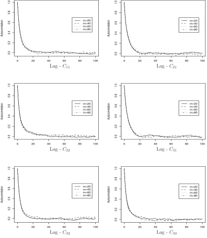
sampler used for the path updates was 98.14%, raising no concerns regarding its performance. Figure
1 shows autocorrelation plots for the posterior draws of theCmatrix components. There is no sign of
any increase to raise suspicions against the irreducibility of the chain. Figure 2 depicts density plots
for some parameters as well as the log-likelihood which may be seen as an appropriate diagnostic plot
for the quality of the approximations. Densities form= 60 andm= 80 look similar and therefore the
argument that their level of augmentation is sufficient appears to be plausible. The plots of Figure 2
and the results of Table 1, which contains summaries of the parameter posterior draws for m= 80,
are in good agreement with the true values of the parameters.
[Figure 1 about here.]
[Figure 2 about here.]
[Table 1 about here.]
6
Application: EUR/USD and GBP/USD exchange rates
The dataset consists of roughly two years of daily exchange EUR/USD and GBP/USD rates,
specif-ically from the 3rd of January 2005 to 22nd of December 2006. We denote these rates with reur/usd
andrgbp/usdand their logarithms withYeur/usdandYgbp/usdrespectively. Our dataset also contains
the corresponding month implied volatilities constructed from options made on the currency pairs.
The data are plotted in Figure 3.
[Figure 3 about here.]
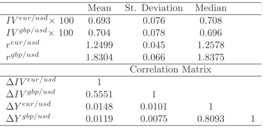
We use the implied volatilities of the currency pairs to construct proxies for their actual volatilities,
denoted withIVeur/usdandIVgbp/usd. For simplicity, these proxies are assumed to be exact
and Kimmel, 2005), or a formulation with noisy observations. Table 2 provides several descriptive
statistics including the correlation matrix of the 4−dimensional time series containing the implied
volatilities and the log-exchange ratesY = IVeur/usd, IVgbp/usd, Yeur/usd, Ygbp/usd
.
[Table 2 about here.]
Note that some correlations appear to be substantial and should be taken into account in the analysis
of the data. Hence we fit the bivariate Heston model to the 4−dimensional time series Y using the
MCMC data augmentation scheme of this paper. Section 3.4 provides details on the reparametrised
likelihood for the data. For reasons of model parsimony, we only consider correlations between the
pairs IVeur/usd, IVgbp/usd
and Yeur/usd, Ygbp/usd
, and set the remaining ones (ρ31,ρ32,ρ41,ρ42)
to zero. This is in line with Table 2 and some preliminary analysis which considered all possible
correlations. Note that the parameters ofC that need to be updated are justC11,C21,C22andC43,
as C33 and C44 are redundant and the remaining entries are equal to zero like the corresponding
correlations. In other words, there exists a 1-1 mapping between the diffusion matrix elements
(σ1,σ2,ρ21,ρ43) and (C11,C21,C22,C43). We complete the model by assigning non-informative priors
as in the previous section: p(θ)∝θ−1for the positive parameters (κ
1,κ2,µ1,µ2,C11,C22) andp(θ)∝1
for the rest (µ3,µ4,C21,C43).
As before, several MCMC runs with different numbers of imputed pointsm={10,20,40}were used.
The data, referring to business days, were assumed to be equidistant and the time was measured
in years. Again, the acceptance rate of the independence sampler used for the path updates was
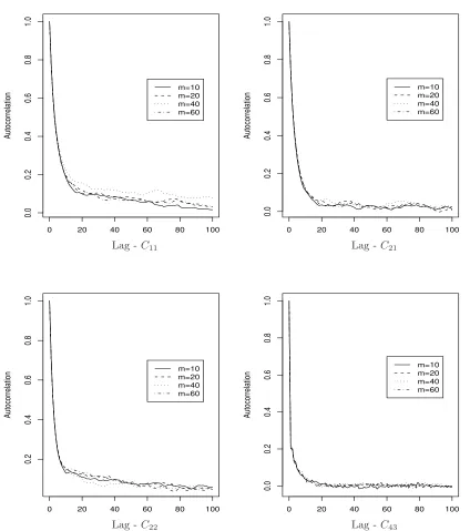
particularly high 99.16%. The autocorrelation plots of draws from the posterior of the parameters
C11,C21,C22, andC43, in Figure 4, reveal no sign of any increase in the level of augmentation.
[Figure 4 about here.]
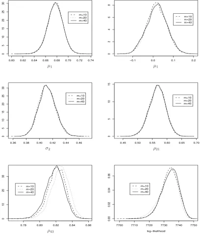
Regarding the approximation error due to the discretisation of the diffusion path, the density plots
from the posterior draws of some parameters and the log-likelihood, in Figure 5, provide convergence
evidence for the approximating sequence of the data augmentation scheme.
Table 3 contains summaries of the parameter posterior draws, where both correlations appear to be
high. Note that the non-parametric estimates of Table 2 are based on the quadratic variation process
and are therefore amenable to bias due to the discretisation of the diffusion path. On the other
hand, the discretisation error of the model estimates may become arbitrary small. The posterior
mean or median values provide point estimates of the parameters which may be used for option
pricing purposes. Alternatively, the samples from their posterior of the parameters may be used in a
Bayesian option pricing framework. In any case, it may be useful to take into account the correlated
market structure of the log-exchange rate and their impled volatilities.
[Table 3 about here.]
7
Discussion
In this paper we introduced a parametrisation framework based on the Cholesky decomposition, for
handling correlations of multi-dimensional diffusions in a Bayesian MCMC setting. This framework
facilitates componentwise updates of the diffusion matrix, in a way so that its positive definite
struc-ture is preserved. It may therefore be of substantial value in high dimensional diffusion models.
The Cholesky factorisation was used in connection with data augmentation and therefore applies to
both directly and partially observed diffusions. In order to overcome degenerate MCMC algorithms,
the likelihood reparametrisation of Roberts and Stramer (2001) was generalised to several
multi-dimensional diffusions, including stochastic volatility models, thus providing a stand alone solution
to the problem. Being a data augmentation scheme, our MCMC algorithm is based on an
approxi-mation of the likelihood, whose error may become arbitrarily small by simply increasing the level of
augmentation.
Nonetheless, the Cholesky factorisation of the diffusion matrix may be coupled with alternative,
to data augmentation, techniques for approximating the likelihood. The exact inference framework
of Beskos et al. (2006a) and the analytic likelihood expansions of A¨ıt-Sahalia (2005) provide such
of the diffusion path, whereas the latter provides closed form expressions of the likelihood. On the
other hand, their generalisation to partially observed diffusion may present major difficulties.
Apart from the updates of the diffusion matrix parameters, our MCMC algorithm differs from
other data augmentation schemes, such as those of Chib et al. (2005) and Golightly and Wilkinson
(2007), in the proposal distribution of the independence sampler involved in the updates of the
diffusion paths. Under these schemes, the proposal may either be the multi-dimensional bridge of
the of Durham and Gallant (2002), or alternatively that of Delyon and Hu (2007), with the target
diffusion matrix. Current work investigates the behavior of all existing approaches in different settings
regarding the dimensionality of the diffusion, the amount of correlation, and the sparseness of the
data.
8
Acknowledgements
Part of the work was carried out during a visit to Lancaster funded through the EU Marie Curie
training scheme. The data of Section 6 were used with the kind permission of Citigroup.
References
A¨ıt-Sahalia, Y. (2005). Closed form likelihood expansions for multivariate diffusions. Annals of
Statistics. To appear.
A¨ıt-Sahalia, Y. and Kimmel, R. (2005). Maximum likelihood estimation for stochastic volatility
models. Journal of Financial Economics. To appear.
Beskos, A., Papaspiliopoulos, O., Roberts, G., and Fearnhead, P. (2006a). Exact and computationally
efficient likelihood-based estimation for discretely observed diffusion processes (with discussion).
Journal of the Royal Statistical Society: Series B (Statistical Methodology), 68(3):333–382.
Beskos, A., Roberts, G. O., Stuart, A., and Voss, J. (2006b). A MCMC method for diffusion bridges.
Submitted.
objective and risk neutral measures for the purposes of options valuation. Journal od Financial
Economics, 56:407–458.
Chib, S., Pitt, M. K., and Shephard, N. (2005). Likelihood based inference for diffusion models.
Submitted.
Cox, J. C., Ingersoll, J. E., and Ross, S. A. (1985). A theory of the term structure of interest rates.
Econometrica, 53:385–407.
Daniels, M. and Kass, R. (1999). Nonconjugate bayesian estimation of covariance matrices in
hierar-chical models. Journal of the American Statistical Association, 94:1254–1263.
Delyon, B. and Hu, Y. (2007). Simulation of conditioned diffusions and applications to parameter
estimation. Stochastic Processes and Application. To appear.
Durham, G. B. and Gallant, A. R. (2002). Numerical techniques for maximum likelihood estimation
of continuous-time diffusion processes. Journal of Business & Economic Statistics, 20(3):297–316.
With comments and a reply by the authors.
Elerian, O. S., Chib, S., and Shephard, N. (2001). Likelihood inference for discretely observed
non-linear diffusions. Econometrica, 69:959–993.
Eraker, B. (2001). Markov chain Monte Carlo analysis of diffusion models with application to finance.
Journal of Business & Economic Statistics, 19(2):177–191.
Ghysels, E., Harvey, A., and Renault, E. (1996). Stochastic volatily, in. Handbook of Statistics 14,
Statistical Methods in Finance. G.S. Maddala and C.R. Rao (eds), North Holland, Amsterdam.
Golightly, A. and Wilkinson, D. (2006). Bayesian sequential inference for nonlinear multivariate
diffusions. Statistics and Computing, 16:323–338.
Golightly, A. and Wilkinson, D. (2007). Bayesian inference for nonlinear multivariate diffusions
observed with error. Computational Statistics and Data Analysis. In press.
Heston, S. (1993). A closed-form solution for options with stochastic volatility. with applications to
Hull, J. C. and White, A. D. (1987). The pricing of options on assets with stochastic volatilities.
Journal of Finance, 42(2):281–300.
Jones, C. S. (1999). Bayesian estimation of continuous-time finance models. Unpublished paper,
Simon School of Business, University of Rochester.
Kalogeropoulos, K. (2007). Likelihood based inference for a class of multidimensional diffusions with
unobserved paths. Journal of Statistical Planning and Inference, 137:3092–3102.
Kalogeropoulos, K., Roberts, G., and Dellaportas, P. (2007). Inference for stochastic volatility models
using time change transformations. Submitted.
Pedersen, A. R. (1995). A new approach to maximum likelihood estimation for stochastic
differ-ential equations based on discrete observations. Scandinavian Journal of Statistics. Theory and
Applications, 22(1):55–71.
Pinheiro, J. and Bates, D. (1996). Unconstrained parametrizations for variance-covariance matrices.
Statistics and Computing, 6(3):289–296.
Roberts, G. and Stramer, O. (2001). On inference for partial observed nonlinear diffusion models
using the metropolis-hastings algorithm. Biometrika, 88(3):603–621.
Rogers, L. C. G. and Williams, D. (1994). Diffusions, Markov processes and martingales, 2, Ito
calculus. Wiley, Chicester.
Sørensen, H. (2004). Parametric inference for diffusion processes observed at discrete points in time:
a survey. International Statistical Review, 72(3):337–354.
Stein, E. M. and Stein, J. C. (1991). Stock proce distributions with stochastic volatility: an analytic
approach. Review of Financial Studies, 4(4):727–752.
Tanner, M. A. and Wong, W. H. (1987). The calculation of posterior distributions by data
A
Proofs of propositions
Proof of proposition 3.1:
The proof is based on he reducibility condition of (11), for which we need the inverse of Σ(Xt, θ)
Σ(Xt, θ)−1 = (Fx(Xt, θ)C)−1 = C−1Fx(Xt, θ)−1.
In coordinate form the above writes
[Σ(Xt, θ)−1]ij = [C−1]ijf{j}(x{tj}, θ)−1, ∀i, j∈ {1, . . . , d}.
Hence, it is not hard to see that the reducibility condition of A¨ıt-Sahalia (2005) holds because
∂[Σ(Xt, θ)−1]ij
∂x{tk}
= ∂[Σ(Xt, θ) −1]
ik
∂x{tj}
= 0, ∀i, j, k∈ {1, . . . , d}, withj < k
Proof of proposition 3.2:
The diffusion matrix of Ut should be ad−dimensional identity matrix, therefore by Ito’s lemma we
get
∇H(Xt, θ)A(∇H(Xt, θ))′ = Id (21)
Consider a transformation of the form
H(Xt, θ) = B Gx(Xt, θ),
where B is an arbitraryd×dmatrix, independent ofXt.
We can write
∇H(Xt, θ) = B DG(Xt, θ),
where DG(Xt, θ) is a diagonal matrix with
Indeed, the k−th row of∇H(Xt, θ) equals
∇H(Xt, θ) =∇
d
X
j=1
Bkjg{i}(xt{j}, θ)
= (Bk1, . . . , Bkd) DG(Xt, θ).
If we substitute on (21), using also (10), we get
B DG(Xt, θ)Fx(Xt, θ)C C′ Fx(Xt, θ)DG(Xt, θ)B′ = Id,
which since DG(Xt, θ)Fx(Xt, θ) = Fx(Xt, θ)DG(Xt, θ) = Id becomes
B C C′B′ = Id,
List of Figures
1 Autocorrelation plots for the posterior draws of the C matrix entries for different numbers of imputed points (m= 20,40,60,80). Simulated data. . . 28 2 Kernel densities of the posterior draws for some parameters (µ1, σ2,ρ32) and the
log-likelihood, for different numbers of imputed points (m = 20,40,60,80). Simulated data. . . 29 3 Daily EUR/USD and GBP/USD rates (up) and their month implied volatilities (%)
(down) from 3rd of January 2005 to 22nd of December 2006. . . 30 4 Autocorrelation plots for the posterior draws of the C matrix entries for different
numbers of imputed points (m = 10,20,40). EUR/USD and GBP/USD exchange rates dataset. . . 31 5 Kernel densities of the posterior draws for some parameters (µ1,µ1,σ2,ρ21,ρ43) and
0 20 40 60 80 100 0.0 0.2 0.4 0.6 0.8 1.0 Autocorrelation m=20 m=40 m=60 m=80
0 20 40 60 80 100
0.0 0.2 0.4 0.6 0.8 1.0 Autocorrelation m=20 m=40 m=60 m=80
0 20 40 60 80 100
0.0 0.2 0.4 0.6 0.8 1.0 Autocorrelation m=20 m=40 m=60 m=80
0 20 40 60 80 100
0.0 0.2 0.4 0.6 0.8 1.0 Autocorrelation m=20 m=40 m=60 m=80
0 20 40 60 80 100
0.0 0.2 0.4 0.6 0.8 1.0 Autocorrelation m=20 m=40 m=60 m=80
0 20 40 60 80 100
0.0 0.2 0.4 0.6 0.8 1.0 Autocorrelation m=20 m=40 m=60 m=80
Lag -C11 Lag -C21
Lag -C22 Lag -C31
[image:29.595.90.509.172.653.2]Lag -C32 Lag -C33
2.0 2.5 3.0 3.5
0.0
0.5
1.0
1.5
2.0
2.5
m=20 m=40 m=60 m=80
0.30 0.35 0.40 0.45
0
5
10
15
20
25
30
m=20 m=40 m=60 m=80
0.4 0.5 0.6 0.7
0
2
4
6
8
10
12
m=20 m=40 m=60 m=80
−550 −540 −530 −520
0.00
0.02
0.04
0.06
0.08
0.10
log−likelihood m=20
m=40 m=60 m=80
µ1 σ2
[image:30.595.107.505.168.648.2]ρ32
Figure 2: Kernel densities of the posterior draws for some parameters (µ1, σ2, ρ32) and the
0 100 200 300 400 500
1.2
1.4
1.6
1.8
2.0
Business Days from January 3rd 2005
Currency Pair
EUR / USD GBP / USD
0 100 200 300 400 500
5
6
7
8
9
10
11
12
Business Days from January 3rd 2005
Month Implied Volatility (%) of the Currency Pair
[image:31.595.89.502.121.718.2]EUR / USD GBP / USD
0 20 40 60 80 100
0.0
0.2
0.4
0.6
0.8
1.0
Autocorrelation
m=10 m=20 m=40 m=60
0 20 40 60 80 100
0.0
0.2
0.4
0.6
0.8
1.0
Autocorrelation
m=10 m=20 m=40 m=60
0 20 40 60 80 100
0.2
0.4
0.6
0.8
1.0
Autocorrelation
m=10 m=20 m=40 m=60
0 20 40 60 80 100
0.0
0.2
0.4
0.6
0.8
1.0
Autocorrelation
m=10 m=20 m=40 m=60
Lag - C11 Lag -C21
[image:32.595.88.512.166.645.2]Lag - C22 Lag -C43
0.60 0.62 0.64 0.66 0.68 0.70 0.72 0.74 0 5 10 15 20 25 30 m=10 m=20 m=40
−0.1 0.0 0.1 0.2
0 2 4 6 8 m=10 m=20 m=40
0.36 0.38 0.40 0.42 0.44 0.46
0 5 10 15 20 25 30 m=10 m=20 m=40
0.45 0.50 0.55 0.60 0.65 0.70
0 5 10 15 m=10 m=20 m=40
0.78 0.80 0.82 0.84 0.86
0 10 20 30 m=10 m=20 m=40
7700 7710 7720 7730 7740 7750
0.00 0.02 0.04 0.06 log−likelihood m=10 m=20 m=40 µ1 µ1
σ2 ρ21
[image:33.595.102.512.166.651.2]ρ43
Figure 5: Kernel densities of the posterior draws for some parameters (µ1,µ1,σ2,ρ21, ρ43) and the
List of Tables
1 Summaries of the posterior draws of the model parameters for m = 80. Simulated dataset. . . 34 2 Descriptive statistics for EUR/USD and GBP/USD exchange rates and their implied
volatilities. . . 35 3 Summaries of the posterior draws of the model parameters for m = 60. EUR/USD
Parameter True Value Posterior mean Posterior SD Posterior median
κ1 0.2 0.174 0.025 0.174
κ2 0.15 0.123 0.031 0.121
κ3 0.22 0.223 0.030 0.224
µ1 2.5 2.578 0.167 2.571
µ2 3.0 2.986 0.366 2.951
µ3 2.0 1.908 0.094 1.905
σ1 0.45 0.434 0.016 0.434
σ2 0.35 0.372 0.012 0.372
σ3 0.4 0.401 0.014 0.402
ρ21 0.45 0.480 0.034 0.480
ρ31 0.35 0.318 0.041 0.319
[image:35.595.89.451.329.487.2]ρ32 0.55 0.537 0.033 0.538
Mean St. Deviation Median
IVeur/usd×100 0.693 0.076 0.708
IVgbp/usd
×100 0.704 0.078 0.696
reur/usd 1.2499 0.045 1.2578
rgbp/usd 1.8304 0.066 1.8375
Correlation Matrix
∆IVeur/usd 1
∆IVgbp/usd 0.5551 1
∆Yeur/usd 0.0148 0.0101 1
[image:36.595.89.355.338.468.2]∆Ygbp/usd 0.0119 0.0075 0.8093 1
Parameter Posterior mean Posterior SD Posterior median
κ1 0.153 0.023 0.153
κ2 0.206 0.030 0.204
µ1 ×100 0.677 0.014 0.677
µ2 ×100 0.689 0.012 0.690
µ3 0.001 0.053 0.001
µ4 0.019 0.049 0.019
σ1×100 0.343 0.010 0.343
σ2×100 0.411 0.013 0.411
ρ21 0.567 0.028 0.567
ρ43 0.821 0.011 0.821