Satisfaction approval voting
Brams, Steven J and Kilgour, D. Marc
New York University, Wilfrid Laurier University
April 2010
Online at
https://mpra.ub.uni-muenchen.de/22709/
Satisfaction Approval Voting
Steven J. Brams
Department of Politics
New York University
New York, NY 10012
USA
D. Marc Kilgour
Department of Mathematics
Wilfrid Laurier University
Waterloo, Ontario N2L 3C5
CANADA
Abstract
We propose a new voting system, satisfaction approval voting (SAV), for
multiwinner elections, in which voters can approve of as many candidates or as many
parties as they like. However, the winners are not those who receive the most votes, as
under approval voting (AV), but those who maximize the sum of the satisfaction scores
of all voters, where a voter’s satisfaction score is the fraction of his or her approved
candidates who are elected. SAV may give a different outcome from AV—in fact, SAV
and AV outcomes may be disjoint—but SAV generally chooses candidates representing
more diverse interests than does AV (this is demonstrated empirically in the case of a
recent election of the Game Theory Society). A decision-theoretic analysis shows that all
strategies except approving of a least-preferred candidate are undominated, so voters will
often find it optimal to approve of more than one candidate. In party-list systems, SAV
apportions seats to parties according to the Jefferson/d’Hondt method with a quota
constraint, which favors large parties and gives an incentive to smaller parties to
coordinate their policies and forge alliances, even before an election, that reflect their
Satisfaction Approval Voting1
1. Introduction
Approval voting (AV) is a voting system in which voters can vote for, or approve
of, as many candidates as they like. Each approved candidate receives one vote, and the
candidates with the most votes win.
This system is well suited to electing a single winner, which almost all the
literature on AV since the 1970s has addressed (Brams and Fishburn, 1978, 1983/2007;
Brams, 2008, chs. 1 and 2). But for multiwinner elections, such as for seats on a council
or in a legislature, AV’s selection of the most popular candidates or parties can fail to
reflect the diversity of interests in the electorate.
As a possible solution to this problem when voters use an approval ballot,2 in
which they can approve or not approve of each candidate, we propose satisfaction
approval voting (SAV). SAV works as follows when the candidates are individuals. A
voter’s satisfaction score is the fraction of his or her approved candidates who are
elected, whether the voter is relatively discriminating (i.e., approves of few candidates) or
not (approves of many candidates). In particular, it offers a strategic choice to voters,
who may bullet vote (i.e., exclusively for one candidate) or vote for several candidates,
perhaps hoping to make a specific set of candidates victorious.
1 We thank Joseph N. Ornstein and Erica Marshall for valuable research assistance, and Richard F. Potthoff
for help with computer calculations that we specifically acknowledge later.
2 Merrill and Nagel (1987) were the first to distinguish between approval balloting, in which voters can
If a fixed number of candidates, say k, is to be elected, SAV chooses the set that
maximizes the sum of all voters’ satisfaction scores. As we will show, SAV may give
very different outcomes from AV; SAV outcomes are not only more satisfying to voters
but also tend to be more representative of the diversity of interests in an electorate.
Moreover, they are easy to calculate.
In section 2, we apply SAV to the election of individual candidates (e.g., to a
council) when there are no political parties. We show, in the extreme, that SAV and AV
may elect disjoint subsets of candidates. When they differ, SAV winners will generally
represent the electorate better—by at least partially satisfying more voters—than AV
winners. While maximizing total voter satisfaction, however, SAV may not maximize
the number of voters who approve of at least one winner—one measure of
representativeness—though it is more likely to do so than AV.
This is shown empirically in section 3, where SAV is applied to the 2003 Game
Theory Society (GTS) election of 12 new Council members from a list of 24 candidates
(there were 161 voters). SAV would have elected two winners different from the 12
elected under AV and would have made the Council more representative of the entire
electorate. We emphasize, however, that GTS members might well have voted
differently under SAV than under AV, so one cannot simply extrapolate a reconstructed
outcome, using a different aggregation method, to predict the consequences of SAV.
In section 4, we consider the conditions under which, in a 3-candidate election
with 2 candidates to be elected, a voter’s ballot might change the outcome, either by
making or breaking a tie. In our decision-theoretic analysis of the 19 contingencies in
outcome in about the same number of contingencies as bullet voting, even though a voter
must split his or her vote when voting for 2 candidates. More general results on optimal
voting strategies under SAV are also discussed.
In section 5, we apply SAV to party-list systems, whereby voters can approve of as
many parties as they like. Parties nominate their “quotas,” which are based on their vote
shares, rounded up; they are allocated seats to maximize total voter satisfaction, measured
by the fractions of nominees from voters’ approved parties that are elected. We show
that maximizing total voter satisfaction leads to the proportional representation (PR) of
parties, based on the Jefferson/d’Hondt method of apportionment, which favors large
parties.
SAV tends to encourage multiple parties to share support, because they can win
more seats by doing so. At the same time, supporters of a party diminish its individual
support by approving of other parties, so there is a trade-off between helping a favorite
party and helping a coalition of parties that may be able to win more seats in toto. Some
voters may want to support only a favorite party, whereas others may want to support
multiple parties that, they hope, will form a governing coalition. We argue that this
freedom is likely to make parties more responsive to the wishes of their supporters with
respect to (i) other parties with which they coalesce and (ii) the candidates they choose to
nominate.3
In section 6, we conclude that SAV may well induce parties to form coalitions, if
not merge, before an election. This will afford voters the ability better to predict what
policies the coalition will promote, if it forms the next government, and, therefore, to vote
3 The latter kind of responsiveness would be reinforced if voters, in addition to being able to approve of
more knowledgeably.4 In turn, it gives parties a strong incentive to take careful account
of their supporters’ preferences, including their preferences for coalitions with other
parties.
2. Satisfaction Approval Voting for Individual Candidates
We begin by applying SAV to the election of individual candidates, such as to a
council or legislature, in which there are no political parties. We assume in the
subsequent analysis that there are at least two candidates to be elected, and more than this
number run for office (to make the election competitive).
To define SAV formally, assume that there are m > 2 candidates, numbered 1, 2,
…, m. The set of all candidates is {1, 2, …, m} = [m], and k candidates are to be elected,
where 2 ≤k < m. Assume voter i approves of a subset of candidates , where V
i
≠ Ø. (Thus, a voter may approve of only 1 candidate, though more are to be elected.)
For any subset of k candidates, S, voter i’s satisfaction is , or the fraction of his or
her approved candidates that are elected. SAV elects a subset of k candidates that
maximizes
(1)
which we interpret as the total satisfaction of voters for S.
4 More speculatively, SAV may reduce a multiparty system to two competing coalitions of parties. The
To illustrate SAV, assume there are m = 4 candidates, {a, b, c, d}, and 10 voters
who approve of the following subsets:5
4 voters: ab
3 voters: c
3 voters: d.
Assume k = 2 of the 4 candidates are to be elected. AV elects {a,b}, because a and b
receive 4 votes each, compared to 3 votes each that c and d receive. By contrast, SAV
elects {c, d}, because the satisfaction scores of the six different two-winner subsets are as
follows:
s(a,b) = 4(½) + 4(½) = 4
s(a,c) = s(a, d) = s(b,c) = s(b, d) = 4(½) + 3(1) = 5
s(c,d) = 3(1) + 3(1) = 6.
Notice that the election of c and d gives 6 voters full satisfaction of 1, whereas the
election of any other pair of candidates, in which some voters receive partial satisfaction
of ½, yields less total satisfaction.
A candidate’s satisfaction score—as opposed to a voter’s satisfaction score—is the
sum of the satisfaction scores of voters who approve of him or her. For example, if a
candidate receives 3 votes from bullet voters, 2 votes from voters who approve of two
candidates, and 5 votes from voters who approve of three candidates, his or her
satisfaction score is 3(1) + 2(½) + 5(1/3) = 5 2/3.
5 We use ab to indicate the strategy of approving of the subset {a,b}, but we use {a,b} to indicate the
Our first proposition shows that it is not necessary to calculate the satisfaction of
all possible winning subsets of candidates to determine which one maximizes total
satisfaction.
Proposition 1. Under SAV, the k winners are the k candidates whose individual
satisfaction scores are the highest.
Proof. Because it follows from (1) that
Thus, the satisfaction score of subset S, s(S), can be obtained by summing the satisfaction
scores of the individual members of S. Now suppose that s(j) has been calculated for all
candidates j = 1, 2,…, m. Arrange the set of m candidates [m] so that the numbers s(j) are
in descending order. Then the first k candidates in the rearranged sequence are a subset
of candidates that maximizes total voter satisfaction. Q.E.D.
As an illustration of Proposition 1, consider the previous example, in which
s(a) = s(b) = 4(½) = 2
s(c) = s(d) = 3(1) = 3.
Because candidates c and d are the two candidates with the highest satisfaction scores,
they are the winners under SAV.
One consequence of Proposition 1 is a characterization of tied elections: There are
two or more winning subsets if and only if there is a tie between the kth and the (k+1)st
Proposition 1. This follows from the fact that tied subsets must contain the k most
satisfying candidates, but if those in the kth and the (k+1)st positions give the same
satisfaction, a subset containing either would maximize total voter satisfaction. Ties
among three or more sets of candidates are, of course, also possible.
It is worth noting that the satisfaction that a voter derives from getting an approved
candidate elected does not depend on how many of the voter’s other approved candidates
are elected, as some multiple-winner systems that use an approval ballot prescribe.6 This
renders candidates’ satisfaction scores additive: The satisfaction from electing subsets of
two or more candidates is the sum of the candidates’ satisfaction scores. Additivity
greatly facilitates the determination of SAV outcomes when there are multiple winners—
simply choose the subset of individual candidates with the highest satisfaction scores.
The additivity of candidate satisfaction scores reflects SAV’s equal treatment of
voters: Each voter has one vote, which is divided evenly among all his or her approved
candidates. Thus, if two candidates are vying for membership in the elected subset, then
gaining the support of an additional voter always increases a candidate’s score by 1/x,
where x is the number of candidates approved of by that voter. This is a consequence of
the goal of maximizing total voter satisfaction, not an assumption about how approval
votes are to be divided.
6 Two of these systems—proportional AV and sequential proportional AV—assume that a voter’s
satisfaction is marginally decreasing—the more of his or her approved candidates are elected, the less satisfaction the voter derives from having additional approved candidates elected. See
http://www.nationmaster.com/encyclopedia/Proportional-approval-voting
http://www.nationmaster.com/encyclopedia/Sequential-proportional-approval-voting
We next compare the different outcomes that AV and SAV can induce.
Proposition 2. AV and SAV can elect disjoint subsets of candidates.
Proof. This is demonstrated by the previous example: AV elects {a,b}, whereas
SAV elects {c,d}.
For any subset S of the candidates, we say that Srepresents a voter i if and only if
voter i approves of some candidate in S. We now ask how representative is the set of
candidates who win under SAV or AV—that is, how many voters approve of at least one
elected candidate.
SAV winners usually represent at least as many, and often more, voters than the
set of AV winners, as illustrated by the previous example, in which SAV represents 6
voters and AV only 4 voters. SAV winners c and d appeal to distinctive voters, who are
more numerous and so win under SAV, whereas AV winners a and b appeal to the same
voters but, together, receive more approval and so win under AV.
But there are (perhaps unlikely) exceptions:
Proposition 3. An AV outcome can be more representative than a SAV outcome.
Proof. Assume there are m = 5 candidates and 13 voters, who vote as follows:
2 voters: a
5 voters: ab
6 voters: cde.
If 2 candidates are to be elected, the AV outcome is either {a, c}, {a, d}, or {a, e} (7
s(a) = 2(1) + 5(½) = 4½
s(b) = 5(½) = 2½
s(c) = s(d) = s(e) = 6(1/3) = 2.
Thus, whichever of the three AV outcomes is selected, the winners represent all 13
voters, whereas the winners under SAV represent only 7 voters. Q.E.D.
The “problem” for SAV in the forgoing example would disappear if candidates c,
d, and e were to combine forces and became one candidate (say, c), rendering s(c) = 6(1)
= 6. Then the SAV and AV outcomes would both be {a, c}, which would give
representation to all 13 voters. Indeed, as we will show when we apply SAV to party-list
systems in section 5, SAV encourages parties to coalesce to increase their combined seat
share.
But first we consider another possible problem of both SAV and AV.
Proposition 4. There can be subsets that represent more voters than either the
SAV or the AV outcome.
Proof. Assume there are m = 5 candidates and 12 voters, who vote as follows:
4 voters: ab
4 voters: acd
3 voters: ade
1 voter: e.
If 2 candidates are to be elected, the AVoutcome is{a, d} (11 and 7 votes, respectively,
s(a) = 4(½) + 7(1/3) = 4 1/3
s(b) = 4(½) = 2
s(c) = 4(1/3) = 1 1/3
s(d) = 7(1/3) = 2 1/3
s(e) = 3(1/3) + 1(1) = 2.
While subset {a, d} represents 11 of the 12 voters, subset {a, e} represents all 12 voters.
Q.E.D.
Interestingly enough, the so-called greedy algorithm (for representativeness)
would select {a,e}. It works as follows. The candidate who represents the most voters—
the AV winner—is selected first. Then the candidate who represents as many of the
remaining (unrepresented) voters as possible is selected next, then the candidate who
represents as many as possible of the voters not represented by the first two candidates is
selected, and so on. The algorithm ends as soon as all voters are represented, or until the
required number of candidates is selected. In the example used to prove Proposition 4,
the greedy algorithm first chooses candidate a (11 votes) and then candidate e (1 vote).
Given a set of ballots, we say a minimal representative set is a subset of candidates
with the properties that (i) every voter approves at least one candidate in the subset, and
(ii) there are no smaller subsets with property (i). In general, finding a minimal
representative set is computationally difficult.7 Although the greedy algorithm finds a
minimal representative set in the previous example, it is no panacea.
7 Technically, the problem is NP hard (http://en.wikipedia.org/wiki/NP-hard), because it is equivalent to the
hitting-set problem, which is a version of the vertex-covering problem
Proposition 5. SAV can find a minimal representative set when both AV and the
greedy algorithm fail to do so.
Proof. Assume there are m = 3 candidates and 17 voters, who vote as follows:
5 voters: ab
5 voters: ac
4 voters: b
3 voters: c.
If 2 candidates are to be elected, the AVoutcome is {a, b} (a gets 10 and b 9 votes),
which is identical to the subset that the greedy algorithm gives.8 On the other hand, the
SAV outcome is {b, c}, because
s(a) = 5(½) + 5(½) = 5
s(b) = 5(½) + 4(1) = 6½
s(c) = 5(½) + 3(1) = 5½.
Not only does this outcome represent all 17 voters, but it is also the minimal
representative set. Q.E.D.
The greedy algorithm fails to find the minimal representative set in the previous
example because it elects the “wrong” candidate—the AV winner, a—first. Curiously, if
we reduce, by 2 voters each, the numbers of voters voting for the four different subsets of
candidates in this example, we have the following:
candidates—which makes the procedure practical for computing election outcomes when there are many candidates and multiple winners.
8 Candidates a, b, and c receive, respectively, 10, 9, and 8 votes; the greedy algorithm first selects a (10
Proposition 6. SAV, AV, and the greedy algorithm can all fail to find a unique
minimal representative set.
Proof. Assume there are m = 3 candidates and 9 voters, who vote as follows:
3 voters: ab
3 voters: ac
2 voters: b
1 voters: c
AV and the greedy algorithm give {a, b}, as in the previous example, but so does SAV
because
s(a) = 3(½) + 3(½) = 3
s(b) = 3(½) + 2(1) = 3½
s(c) = 3(½) + 1(1) = 2½.
As before, {b, c} is the minimal representative set. Q.E.D.
Minimal representative sets help us assess and compare SAV and AV outcomes of
elections; the greedy algorithm contributes by finding an upper bound on the size of a
minimal representative set, because it eventually finds a set that represents all voters,
even if it is not minimal. But there is a practical problem with basing an election
procedure on the minimal representative set: Only by chance will that set have k
members. If it is either smaller or larger, it must be “adjusted.”
But in what manner? For example, if it is too small, should one add candidates
Or after each voter has approved of at least one winner, should it, like SAV, maximize
total voter satisfaction?
It seems to us that maximizing total voter satisfaction from the start is a simple and
desirable goal, even if doing so does not always give a subset that is as representative as
possible. Also, if one does not divide a voter’s vote equally among multiple candidates
but allows voters who cast more approval votes to weigh in more—as do proportional
AV and sequential proportional AV (see note 6)—clones have an incentive to form.
But it is AV that creates the greatest incentive to form clones, because it gives a
full weight of 1 to every candidate of whom a voter approves. To illustrate this problem,
assume that 2 candidates are to be elected in the following 12-voter, 3-candidate
example:
5 voters: a
4 voters: b
3 voters: c
Under both AV and SAV, {a,b} is elected, representing 9 of the 12 voters. But if
candidate a splits into two clones, a1 and a2, and the 5 supporters of a approve of both
clones, they would win under AV, representing only 5 of the 12 voters. But under SAV,
they would lose, because
s(a1) = s(a2) = 5(½) = 2½
s(b) = 4(1) = 4
Instead, the SAV outcome would be {b,c}, which does represent a majority of 7 of the 12
voters.
Because SAV divides 1 vote equally among all candidates of whom a voter
approves, it discourages the formation of clones. In the previous example, candidate a
would have to receive at least 9 votes in order to make it beneficial for it to split into two
clones, a1 and a2. Now, however, these clones would “deserve” to be the two winners,
because they would be approved of by at least 9 of the 16 voters.
We turn next to a real election, in which AV was used to elect multiple winners,
and assess the possible effects of SAV, had it been used. We are well aware that voters
might have voted differently under SAV and take up this question in section 4.
3. The Game Theory Society Election
In 2003, the Game Theory Society (GTS) used AV for the first time to elect 12
new council members from a list of 24 candidates. (The council comprises 36 members,
with 12 elected each year to serve 3-year terms.9) We give below the numbers of
members who voted for from 1 to all 24 candidates (no voters voted for between 19 and
23 candidates):
Votes cast
1 2 3 4 5 6 7 8 9 10 11 12 13 14 15 16 17 18 24
# of voters
3 2 3 10 8 6 13 12 21 14 9 25 10 7 6 5 3 3 1
9 The fact that there is exit from the council after three years makes the voting incentives different from a
Casting a total of 1574 votes, the 161 voters, who constituted 45 percent of the GTS
membership, approved, on average, 1574/161≈ 9.8 candidates; the median number of
candidates approved of, 10, is almost the same.10
The modal number of candidates approved of is 12 (by 25 voters), echoing the
ballot instructions that 12 of the 24 candidates were to be elected. The approval of
candidates ranged from a high of 110 votes (68.3 percent approval) to a low of 31 votes
(19.3 percent approval). The average approval received by a candidate was 40.7 percent.
Because the election was conducted under AV, the elected candidates were the 12
most approved, who turned out to be all those who received at least 69 votes (42.9
percent approval). Do these AV winners best represent the electorate? With the caveat
that the voters might well have approved of different candidates if SAV rather than AV
had been used, we compare next how the outcome would have been different if SAV had
been used to aggregate approval votes.
Under SAV, 2 of the 12 AV winners would not have been elected.11 Each set of
winners is given below—ordered from most popular on the left to the least popular on the
right, as measured by approval votes—with differences between those who were elected
under AV and those who would have been elected under SAV underscored:
AV: 111111111111000000000000
SAV: 111111111010110000000000
10 Under SAV, whose results we present next, the satisfaction scores of voters in the GTS election are
almost uncorrelated with the numbers of candidates they approved of, so the number of candidates
approved of does not affect, in general, a voter’s satisfaction score—at least if he or she had voted the same as under AV (a big “if” that we investigate later).
11 Under the “minimax procedure” (Brams, Kilgour, and Sanver, 2007; Brams, 2008), 4 of the 12 AV
winners would not have been elected. These 4 include the 2 who would not have been elected under SAV; they would have been replaced by 2 who would have been elected under SAV. Thus, SAV partly
Observe that the AV winners who came in 10th (70 votes) and 12th (69 votes) would have
been displaced under SAV by the candidates who came in 13th (66 votes) and 14th (62
votes), according to AV, and just missed out on being elected.
Recall that a voter is represented by a subset of candidates if he or she approves of
at least one candidate in that subset. The elected subset under SAV represents all but 2 of
the 161 voters, whereas the elected subset under AV failed to represent 5 of the 161
voters. But neither of these subsets is the best possible; the greedy algorithm gives a
subset of 9 candidates that represents all 161 voters, which includes 5 of the AV winners
and 6 SAV winners, including the 2 who would have won under SAV but not under AV.
It turns out, however, that this is not a minimal representative set of winners: There
are more than a dozen subsets with 8 candidates, but none with 7 or fewer candidates,
that represent all 161 voters, making 8 the size of a minimal representative set.12 To
reduce the number of such sets, it seemed reasonable to ask which one maximizes the
minimum satisfaction of all 161 voters.
This criterion, however, was not discriminating enough to produce one subset that
most helped the satisfied voter: There were 4 such subsets that gave the
least-satisfied voter a satisfaction score of 1/8 = 0.125—that is, that elected one of his or her
approved candidates. To select the “best” among these, we used as a second criterion the
one that maximizes total voter satisfaction, which gives
100111000000110001000001.
12 We are grateful to Richard F. Potthoff for writing an integer program that gave the results for the GTS
Observe that only 4 of the 8 most approved candidates are selected; moreover, the
remaining 4 candidates include the least-approved candidate (24th on the list).
But ensuring that every voter approves of at least one winner comes at a cost. The
total satisfaction that the aforementioned minimal representative set gives is 60.9,
whereas the subset of 8 candidates that maximizes total voter satisfaction—without
regard to giving every voter an approved representative—is
111110011000100000000000.
Observe that 6 of the 8 most approved candidates are selected (the lowest candidate is
13th on the list). The total satisfaction of this subset is 74.3, which is a 22 percent
increase over the above score of the most satisfying minimal representative set. We leave
open the question whether such an increase in satisfaction is worth the
disenfranchisement of a few voters.
In choosing a minimal representative set, the size of an elected voting body is
allowed to be endogenous. In fact, it could be as small as one candidate if one candidate
is approved of by everybody.
By contrast, if the size of the winning set is fixed, then once a minimal
representative set has been selected—if that is possible—then one can compute the
larger-than-minimal representative set that maximizes total voter satisfaction. In the case
of the GTS, because there is a minimal representative set with only 8 members, we know
that a 12-member representative set is certainly feasible.
In making SAV and related calculations for the GTS election, we extrapolated
from the AV ballots. We caution that our extrapolations depend on the assumption that
under SAV, would GTS voters have been willing to divide their one vote among multiple
candidates if they thought that their favorite candidate needed their undivided vote to
win?
4. Voting for Multiple Candidates under SAV: A Decision-Theoretic Analysis
To try to answer the forgoing question, we begin by analyzing a much simpler
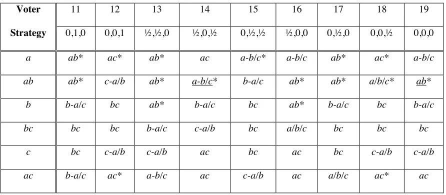
situation—there are 3 candidates, with 2 to be elected. As shown in Table 1, there are
exactly 19 contingencies in which a single voter’s strategy can be decisive—that is, make
a difference in which 2 of the 3 candidates are elected—by making or breaking a tie
among the candidates. In decision theory, these contingencies are the so-called states of
nature.
Table 1 about here
In Table 1, the contingencies are shown as the numbers of votes that separate the
three candidates.13 For example, contingency 4 (1,½,0) indicates that candidate a is
ahead of candidate b by ½ vote, and that candidate b is ahead of candidate c by ½ vote.14
The outcomes produced by a voter’s strategies in the in the left column of Table 1 are
indicated either (i) by the two candidates elected (e.g., ab), (ii) by a candidate followed
13 Notice that the numbers of votes shown in a contingency are all within 1 of each other, enabling a
voter’s strategy to be decisive; these numbers need not sum to an integer, even though the total number of voters and votes sum to an integer. For example, contingency 4 can arise if there are 2 ab voters and 1 ac
voter, giving satisfaction scores of 3/2, 1, and ½, respectively, to a, b, and c, which sum to 3. But this is
equivalent to contingency 4 (1,½,0), obtained by subtracting ½ from each candidate’s score, whose values
do not sum to an integer. Contingencies of the form (1,½,½), while feasible, are not included, because they
are equivalent to contingencies of the form (½,0,0)—candidate a is ½ vote ahead of candidates b and c.
14 We have not shown contingencies in which any candidate is guaranteed a win or a loss. The 19
by two candidates who tie for second place, indicated by a slash (e.g., a-b/c), or (iii) by
all the candidates in a three-way tie (a/b/c).
A voter may choose any one of the six strategies by approving of either one or two
candidates. (Approving of all three candidates, or none at all, would have no effect on
the outcome, so we exclude them as strategies that can be decisive.15) To determine the
optimal strategies of a voter, whom we call the focal voter, we posit that he or she has
strict preference a b c.
We assume that the focal voter has preferences not only for individual candidates
but also over sets of two or three candidates. In particular, given this voter’s strict
preference for individual candidates, we assume the following preference relations for
pairs and triples of candidates:
ab a-b/c ac ≈b-a/c ≈a/b/c c-a/b bc,
where “≈” indicates indifference, or a tie, between pairs of outcomes: One outcome in
the pair is not strictly better than the other. Thus, the certain election of a and c (ac) is no
better nor worse than either the certain election of b and the possible election of either a
or c (b-a/c), or the possible election of any pair of a, b, or c (a/b/c).16
We have starred the outcomes, for each contingency, that are the best or the
tied-for-best for the focal voter; underscores indicate a uniquely best outcome. In contingency
15 If there were a minimum number of votes (e.g., a simple majority) that a candidate needs in order to win,
then abstention or approving of everybody could matter. But here we assume the two candidates with the most votes win, unless there is a tie, in which case we assume there is an (unspecified) tie-breaking rule.
16 Depending on the tie-breaking rule, the focal voter may have strict preferences over these outcomes, too.
Because each allows for the possibility of any pair of winning candidates, we chose not to distinguish them. To be sure, a-b/c (2nd best) and c-a/b (2nd worst) also allow for the possibility of any pair of winning
candidates, but the fact that the first involves the certain election of a, and the second the certain election of
4, for example, there are four starred ab outcomes, all of which give the focal voter’s top
two candidates. These outcomes are associated with the focal voter’s first four strategies;
by contrast, his or her other two strategies elect less preferred sets of candidates.
In contingency 7, outcome ab, associated with the focal voter’s strategy a, is not
only starred but also underscored, because it is a uniquely best outcome. A strategy that
is associated with a uniquely best outcome is weakly undominated, because no other
strategy can give at least as good an outcome for that contingency.
Observe from Table 1 that strategy a leads to a uniquely best outcome in 2
contingencies (3 and 8), strategy ab in 2 contingencies (14 and 19), and strategy b in 1
contingency (7), rendering all these strategies weakly undominated. It is not difficult to
show that the focal voter’s other three strategies, all of which involve approving of c, are
weakly dominated:
• a, ab, and b weakly dominate bc
• a and ab weakly dominate c
• a weakly dominates ac.
In no contingency do the weakly dominated strategies lead to a better outcome than the
strategy by which they are dominated, and in at least one contingency they lead to a
strictly worst outcome.
Among the weakly undominated strategies, a leads to at least a tied-for-best
outcome in 14 contingencies, ab in 13 contingencies (9 of the a and ab contingencies
overlap), and b in 6 contingencies. In sum, it is pretty much a toss-up between weakly
It is no fluke that the focal voter’s three strategies that include voting for candidate
c (c, ac, and bc) are all weakly dominated.
Proposition 7. A strategy that includes approving of a least-preferred candidate
is weakly dominated under SAV, whatever the number of candidates m.
Proof. Let W be a focal voter’s strategy that includes approving of a
least-preferred (“worst”) candidate, w. Let W be the focal voter’s strategy of duplicating W,
except for approving of w, unless W involves voting only for w. In that case, let W be a
strategy of voting for any candidate other than w.
Assume that that the focal voter chooses W. Then Wwill elect the same
candidates that W does except, possibly, for w. However, there will be at least one
contingency in which W does not elect w with certainty (e.g., when w = 0 in the
contingency) and W does, but none in which the reverse is the case. Hence, W weakly
dominates W. Q.E.D.
In Table 1, voting for a second choice, candidate b, is a weakly undominated
strategy, because it leads to a uniquely best outcome in contingency 5. This is not the
case for AV, in which a weakly undominated strategy includes always approving of a
most-preferred candidate—not just never approving of a least-preferred candidate (Brams
and Fishburn, 1978).
Thus, SAV admits more weakly undominated strategies than AV. In some
situations, it may be in the interest of a voter to approve of set of strictly less-preferred
candidates and forsake a set of strictly more-preferred candidates. As a case in point,
candidates are to be elected. In contingency (a, b, c, d, e) = (0, 0, 3/4, 1, 1), strategy ab
elects candidates d and e, the focal voter’s two worst choices, whereas strategy cd,
comprising less-preferred candidates, elects candidates c and d, which is a strictly better
outcome.
To conclude, our decision-theoretic analysis of the 3-candidate, 2-winner case
demonstrates that voting for one’s two most-preferred candidates leads to the same
number of uniquely best and about the same number of at least tied-for-best outcomes,
despite the fact that voters who vote for more than one candidate must split their votes
evenly under SAV. We plan to investigate whether this finding carries over to elections
in which there are more candidates and more winners, as well as the effect that the ratio
of candidates to winners has.
Unlike AV, approving of just a second choice when there are 3 competitive
candidates is a weakly undominated strategy under SAV, though it is uniquely optimal in
only one of the 19 contingencies.17 More generally, while it is never optimal for a focal
voter to select a strategy that includes approving of a worst candidate (not surprising),
sometimes it is better to approve of strictly inferior candidates than strictly superior
candidates (more surprising), though this seems relatively rare.
5. Voting for Political Parties
In most party-list systems, voters vote for political parties, which win seats in a
parliament in proportion to the number of votes they receive. Under SAV, voters would
17 To the degree that voters have relatively complete information on the standing of candidates (e.g., from
not be restricted to voting for one party but could vote for as many parties as they like. If
a voter approves of x parties, each approved party’s score would increase by 1/x.
Unlike standard apportionment methods, some of which we will describe shortly,
SAV does not award seats according to the “quota” to which each party is entitled
(typically, a whole number and a fractional remainder). Instead, parties are allocated
seats to maximize total voter satisfaction, measured by the fractions of nominees from
voters’ approved parties that are elected.
We begin our analysis with an example, after which we formalize the application
of SAV to party-list systems. Then we return to the example to illustrate the effects of
voting for more than one party and a paradox that this may create.
Bullet Voting
SAV assumes that the number of candidates that a party nominates is equal to its
upper quota (its quota rounded up). To illustrate, consider the following 3-party,
11-voter example, in which 3 seats are to be filled (we indicate parties by capital letters).
5 voters support A
4 voters support B
2 voters support C.
Assume that the supporters of each party vote exclusively for it. Party I’s quota,
qi, is its proportion of votes times the number of seats to be apportioned:
qA = (5/11)(3) 1.364
qB = (4/11)(3) 1.091
Under SAV, we assume that each party nominates a number of candidates equal to its
upper quota (i.e., its quota rounded up), so A, B, and C nominate 2, 2, and 1 candidates,
respectively—2 more than the number of candidates to be elected. We emphasize that
the numbers of candidates nominated are not a choice that the parties make but follow
from their quotas, based on the election returns.
SAV finds apportionments of seats to parties that (i) maximize total voter
satisfaction and (ii) are monotonic: A party that receives more votes than another cannot
receive fewer seats.
In our previous example, there are two monotonic apportionments—(2, 1, 0) and
(1, 1, 1) to parties (A, B, C)—giving s values of
s(2, 1, 0) = 5(1) + 4(½) + 2(0) = 7
s(1, 1, 1) = 5(½) + 4(½) + 2(1) = 6½.
Apportionment (2, 1, 0) maximizes s, giving
• 5 A voters satisfaction of 1 for getting A’s 2 nominees elected
• 4 B voters satisfaction of ½ for getting 1 of B’s 2 nominees elected
• 2 C voters satisfaction of 0, because C’s nominee is not elected.
Formalization
In a SAV election of k candidates from lists provided by parties 1, 2, …, p,
suppose that party i has vi supporters. Then party i’s quota is qi=
vi
vj j=1
p
∑
⎡ ⎣ ⎢ ⎢ ⎢ ⎢ ⎤ ⎦ ⎥ ⎥ ⎥ ⎥k. If qi is an
We henceforth assume that all parties’ quotas are nonintegral. Then party i
receives either its lower quota, , or its upper quota, . Of course, ui = li
+ 1. In total, r=k− lj j=1
p
∑
parties receive their upper quota rather than their lower quota.By assumption, r > 0. The set of parties receiving upper quota, S⊆[p] = {1, 2, …, p}, is
chosen to maximize the total satisfaction of all voters, s(S), subject to |S| = r.
Recall that when electing individual candidates, SAV chooses candidates that
maximize total voter satisfaction. When allocating seats to parties, SAV finds
apportionments of seats that maximize total voter satisfaction.
The apportionment in our example is not an apportionment according to the
Hamilton method (also called “largest remainders”), which begins by giving each party
the integer portion of its exact quota (1 seat to A and 1 seat to B). Then any remaining
seats go to the parties with the largest remainders until the seats are exhausted, which
means that that C, with the largest remainder (0.545), gets the 3rd seat, yielding the
apportionment (1, 1, 1) to (A, B, C).
There are five so-called divisor methods of apportionment (Balinski and Young,
1982/2001). Among these, only the Jefferson/d’Hondt method, which is the one that
most favors large parties, gives the SAV apportionment of (2, 1, 0) in our example.18
This is no accident, as shown by the next proposition.
18 The Jefferson/d’Hondt method allocates seats sequentially, giving the next seat to the party that
maximizes v/(a + 1), where v is its number of voters and a is its present apportionment. Thus, the 1st seat
goes to A, because 5 > 4 > 2 when a = 0. Now a = 1 for A and remains 0 for B and C. Because 4/1 > 5/2 > 2/1, B gets the 2nd seat. Now a = 1 for A and B and remains 0 for C. Because 5/2 > 4/2 = 2/1, A gets the 3rd
seat, giving an apportionment of (2, 1, 0) to (A, B, C). The divisor method that next-most-favors large parties is the Webster/Sainte-Laguë method, under which the party that maximizes v/(a + ½) gets the next
seat. After A and B get the first two seats, the 3rd seat goes to C, because 2/(½) > 5/(3/2) > 4/(3/2), so the
Proposition 9. Applied to political parties, SAV gives the same apportionment as
the Jefferson/d’Hondt apportionment method, but with an upper-quota restriction.19 SAV
apportionments also satisfy lower quota and thus satisfy quota.
Proof. Each of party i’s vi voters gets satisfaction of 1 if party i is allocated its
upper quota, and satisfaction li
u
i
if party i is allocated its lower quota. If the subset of
parties receiving upper quota is S⊆[p], then the total satisfaction over all voters is
s(S)= vi i∈S
∑
+ vi i∉S∑
li ui⎛ ⎝
⎜ ⎞⎠⎟ = vi i=1
p
∑
− vi ui i∉S∑
, (2)where the latter equality holds because . The SAV apportionment is,
therefore, determined by choosing S such that |S| = r and S maximizes s(S), which by (2)
can be achieved by choosing Sc = [p] – S to minimize . Clearly, this requirement is
achieved when S contains the r largest values of .
To compare the SAV apportionment with the Jefferson/d’Hondt apportionment,
assume that all parties have already received li seats. The first party to receive ui seats is,
according to Jefferson/d’Hondt, the party, i, that maximizes . After this party’s
allocation has been adjusted to equal its upper quota, remove it from the set of parties.
The next party to receive ui according to Jefferson/d’Hondt is the remaining party with
19 There is an objective function with a min/max operator that Jefferson/d’Hondt also optimizes (Balinski
the greatest value of , and so on. Clearly, parties receive seats in decreasing order of
their values of .
Unlike (unrestricted) Jefferson/d’Hondt apportionments, SAV apportionments
satisfy upper quota, because parties cannot nominate, and therefore cannot receive, more
seats than their quotas rounded up.20 Since Jefferson/d’Hondt apportionments always
satisfy lower quota (Balinski and Young, 1982/2001, pp. 91, 130), SAV apportionments
satisfy quota.21 Q.E.D.
Because SAV produces Jefferson/d’Hondt apportionments, except for the
upper-quota restriction, SAV favors large parties. Nevertheless, small parties will not be wiped
out, provided their quotas are at least 1, unless there is a higher threshold (5 percent of
the vote in several countries) for representation in a parliament.
Multiple-Party Voting
If a voter votes for multiple parties, his or her vote is equally divided among all his
or her approved parties. To illustrate in our previous example, suppose parties B and C
reach an agreement on policy issues, and their 4 and 2 supporters, respectively, approve
of both parties. We suppose that the 5 party A supporters continue to vote for just A.
20 We assume that parties propose an ordering of candidates for their party lists before the election, but
only the results of the election tell them how far down their lists they can go in nominating their upper quotas of candidates.
21 The Jefferson/d’Hondt method with an upper-quota constraint is what Balinski and Young (1982/2001,
Now B and C receive a total of 6(½) = 3 votes each, which are equally divided
between them, making the quotas of the three parties the following:
qA = (5/11)(5) 1.364
qB = (5/11)(3) 0.818
qC = (1/11)(3) 0.818.
These quotas allow for three monotonic apportionments, shown on the left sides of the
equations below, which yield the following satisfaction scores:
s(2, 1, 0) = 5(1) + 6(½) = 8
s(1, 2, 0) = 5(1) + 6(½) = 8
s(1, 1, 1) = 5(½) + 6(1) = 8½ .
Now the SAV apportionment that maximizes satisfaction is (1, 1, 1). Compared with
apportionment (2, 1, 0) earlier with bullet voting, A loses a seat, B stays the same, and C
gains a seat.
A Paradox
Despite the fact that B and C supporters can together ensure themselves of a
majority of 2 seats if they approve of each other’s party, they may still go their separate
ways. The reason is that B does not individually benefit from supporting C; their
supporters would presumably have to be assured that there is collective benefit in
supporting C.
A possible way around this paradox is for B and C to become one party, assuming
Because the combination of B and C has more supporters than A does, this combined
party would win a majority of seats.
6. Conclusions
We have proposed a new voting system, satisfaction approval voting (SAV), for
multiwinner elections. It uses an approval ballot, whereby voters can approve of as many
candidates or parties as they like, but they do not win seats based on the number of
approval votes they receive.
We first considered the use of SAV in elections in which there are no political
parties, such as in electing members of a city council. SAV elects the set of candidates
that maximizes the satisfaction of all voters, where a voter’s satisfaction is the fraction of
his or her approved candidates who are elected. This measure works equally well for
voters who approve of few or of many candidates and, in this sense, can mirror a voter’s
personal tastes.
A candidate’s satisfaction score is the sum of the satisfaction that his or her
election would give to all voters. This is 1/x from a voter who approves of him or her,
where x is the number of candidates approved of by the voter. The winning set of
candidates is the one with the highest individual satisfaction scores.
Among other findings, we showed that SAV and AV may elect disjoint sets of
candidates. SAV tends to elect candidates that give more voters either partial or
complete satisfaction—and thus representation—than does AV, but this is not universally
true and is a question that deserves to be investigated further.
Additionally, SAV inhibits candidates from creating clones to increase their
voter’s satisfaction score will be either 0 or 1), risk-averse voters may be inclined to
approve of multiple candidates.
SAV may not elect a representative set of candidates—whereby every voter
approves of at least one elected candidate—as we showed would have been the case in
the 2003 election of the Game Theory Society Council. However, the SAV outcome
would have been more representative than the AV outcome (given the approval ballots
remained the same as in the AV election). Yet we also showed that a fully representative
outcome could have been achieved with a smaller subset of candidates (8 instead of 12).
Because SAV divides a voter’s vote evenly among the candidates he or she
approves of, SAV may encourage more bullet voting than AV does. However, we
showed that in 3-candidate, 2-winner elections, voters would find it almost equally
attractive to approve of their two best choices as their single best choice. Unlike AV,
they may vote for strictly less-preferred candidates if they think their more-preferred
candidates cannot benefit from their help.
We think the most compelling application of SAV is to party-list systems. Each
party would provide an ordering of candidates on its party list before the election, but it
would be able to nominate only a number of candidates equal to its upper quota after the
election. The candidates elected would be those that maximize total voter satisfaction
among monotonic apportionments.
Because parties nominate, in general, more candidates than there are seats to be
filled, not every voter can be completely satisfied. We showed that the apportionment of
quota constraint, which tends to favor larger parties while still ensuring that smaller
parties receive at least their lower quotas.
To analyze the effects of voting for multiple parties, we compared a scenario in
which voters bullet voted with a scenario in which they voted for multiple parties.
Individually, parties are hurt when their supporters approve of other parties. Collectively,
however, they may be able to increase their combined seat share by forming coalitions—
whose supporters approve all parties in it—or even by merging. At a minimum, SAV
would discourage parties from splitting up unless to do so would mean they would be
able to recombine to form a new and larger party, as Kadima did in Israel.
Normatively speaking, we believe that better coordination by parties should be
encouraged, because it would give voters a clearer idea of what to expect when they
decide which parties to support—compared to the typical situation today, when voters
can never be sure about what parties will join in a governing coalition and what its
policies will be. Because this coordination makes it easier for voters to know what
parties to approve of, and for party coalitions to form that reflect their supporters’
interests, we believe that SAV is likely to lead to more informed voting and more
Table 1
Strategies and Outcomes for19 Contingencies in 3-Candidate, 2-Winner Elections in Which One Voter Can Be Decisive
Contingency
Voter 1 2 3 4 5 6 7 8 9 10
Strategy 1,1,0 1,0,1 0,1,1 1,½,0 1,0,½ ½,1,0 0,1,½ ½,0,1 0, ½,1 1,0,0
a ab* ac* a-b/c* ab* ac ab* ab* ac* ac* a-b/c
ab ab* ac* bc ab* a-b/c ab* b- a/c ac* bc ab*
b ab* a/b/c* bc ab* ab* ab* bc bc bc ab*
bc ab* ac* bc ab* ac b-a/c bc c-a/b bc a-b/c
c a/b/c ac* bc ac ac bc bc ac bc ac
ac ab* ac* bc a-b/c ac ab* bc ac c-a/b ac
Contingency (cont.)
Voter 11 12 13 14 15 16 17 18 19
Strategy 0,1,0 0,0,1 ½,½,0 ½,0,½ 0,½,½ ½,0,0 0,½,0 0,0,½ 0,0,0
a ab* ac* ab* ac a-b/c* a-b/c ab* ac* a-b/c
ab ab* c-a/b ab* a-b/c* b-a/c ab* ab* a/b/c* ab*
b b-a/c bc ab* b-a/c bc ab* b-a/c bc b-a/c
bc bc bc b-a/c c-a/b bc a/b/c bc bc bc
c bc c-a/b c-a/b ac bc ac bc c-a/b c-a/b
ac b-a/c ac* a-b/c ac c-a/b ac a/b/c ac* ac
Note: The outcomes produced by a voter’s strategies in the left columns of Table 1 are indicated (i) by the two candidates elected (e.g., ab), (ii) by a candidate followed by two candidates who tie for second place, separated by a slash (e.g., a-b/c), or (iii) the
candidates in a three-way tie (a/b/c). For the focal voter with preference a b c,
References
Alcalde-Unzu, Jorge, and Marc Vorsatz (2009). “Size Approval Voting.” Journal of
Economic Theory 144, no. 3 (May): 1187-1210.
Balinski, M. L., and H. P. Young (1978). “Stability, Coalitions and Schisms in
Proportional Representation Systems.” American Political Science Review 72,
no. 3 (September): 848-858.
Balinski, Michel L., and H. Peyton Young (1982/2001). Fair Representation: Meeting
the Ideal of One Man, One Vote. New Haven, CT/Washington, DC: Yale
University Press/Brookings Institution.
Barberà, S., M. Maschler, and J. Shalev (2001). “Voting for Voters: A Model of
Electoral Evolution.” Games and Economic Behavior 37, no. 1 (October): 40-78.
Brams, Steven J. (2008). Mathematics and Democracy: Designing Better Voting and
Fair-Division Procedures. Princeton, NJ: Princeton University Press.
Brams, Steven J., and Peter C. Fishburn (1978). “Approval Voting.” American Political
Science Review 72, no. 3 (September): 831-847.
Brams, Steven J., and Peter C. Fishburn (1983/2007). Approval Voting. New York:
Springer.
Brams, Steven J., D. Marc Kilgour, and M. Remzi Sanver (2007). “A Minimax
Procedure for Electing Committees.” Public Choice 132, nos. 3-4 (September):
401-420.
Karp, Richard M. (1972). “Reducibility among Combinatorial Problems.” In R. E.
Miller and J. W. Thatcher (eds.), Complexity of Computer Calculations. New
Kilgour, D. Marc (2010). “Using Approval Balloting in Multi-Winner Elections.”
In Jean-François Laslier and M. Remzi Sanver (eds.), Handbook of Approval
Voting. Berlin: Springer.
Merrill, Samuel, III, and Jack H. Nagel (1987). “The Effect of Approval Balloting on
Strategic Voting under Alternative Decision Rules.” American Political Science
Review 81, no. 2 (June): 509-524.
Still, J. W. (1979). “A Class of New Methods for Congressional Apportionment.” SIAM