http://dx.doi.org/10.4236/tel.2016.63056
How to cite this paper: Hefti, A. (2016) Symmetric Stability in Symmetric Games. Theoretical Economics Letters, 6, 488-493. http://dx.doi.org/10.4236/tel.2016.63056
Symmetric Stability in Symmetric Games
Andreas HeftiSchool of Management and Law, University of Zurich, Winterthur,Switzerland
Received 29 March 2016; accepted 6 June 2016; published 9 June 2016
Copyright © 2016 by author and Scientific Research Publishing Inc.
This work is licensed under the Creative Commons Attribution International License (CC BY). http://creativecommons.org/licenses/by/4.0/
Abstract
The idea of symmetric stability of symmetric equilibria is introduced which is relevant, e.g., for the comparative-statics of symmetric equilibria with symmetric shocks. I show that symmetric stabil-ity can be expressed in a two-player reduced-form version of the N-player game, derive an ele-mentary relation between symmetric stability and the existence of exactly one symmetric equili-brium, and apply symmetric stability to a two-dimensional N-player contest.
Keywords
Symmetric Games, Symmetric Equilibrium, Stability, Uniqueness
1. Introduction
489
2. Symmetric Games
I consider games of N ≥2 players. xg≡
(
xg1,,xgk)
∈S k( )
is a strategy of player g, where( )
1 ki i
S≡S k = ×=S with Si =0,Si⊂, Si>0, and interior Int S
( )
i . All players have identical strategy space. The payoff of g is represented by a C2 function Πg(
x1,,xg,,xN)
≡ Π(
xg,x−g)
, which is strongly quasiconcave1 in xg. In a symmetric game all players have identical payoff function in the sense that(
)
( )( ) ( ) ( )
(
)
1, , , , 1, , , ,
g g
g N g N
x x x σ xσ xσ xσ
Π = Π
for any permutation σ of
{
1,,N}
. With the above assumptions, player g’s best-reply function( )
g( )
g g
x x
ϕ − ≡ϕ − is continuous, and differentiable at interior points. Given the focus on symmetric equilibria one can restrict attention to a reduced-form problem by picking an indicative player (g=1), and requiring all opponents to play the same strategies, i.e.x−1=
(
x,,x)
, x∈S. Let Π(
x x1,)
≡ Π(
x x1, −1)
with correspond- ing best-reply ϕ( )
x ≡ϕ( )
x−1 and derivative ∂ϕ( )
x . Any symmetric equilibrium*
x is identifiable by its first projection x1*∈S,
*
x is a symmetric equilibrium if *
( )
*1 1
x =ϕ x , a symmetric equilibrium always exists and the set of symmetric equilibria is compact [1].
2.1. Symmetric Stability
I mostly restrict attention to the system of gradient dynamics2
( )
, 1 jj j
x = ∇ ΠS x ≤ ≤j N (1)
where S is a k×k positive-diagonal adjustment matrix, and
( )
( )
j j j j x x x ∂Π∇ Π =
∂ . A solution to (1) has the form
( )
(
( )
)
1
j j N
x t = x t ≤ ≤ , where xj
( )
t =(
xj1( )
t ,,xjk( )
t)
is the trajectory of j. I consider a restricted version of this trajectory map, where initial values x( )
0 are symmetric, i.e. x1( )
0 ==xN( )
0 . Then, by symmetry,( )
j
x t is the same for all players and solves
( )
( )
(
)
1
1
1 1 1
1
, , where
x x x x
x S x x
x =
∂Π
= ∇Π ∇Π ≡
∂
(2)
I say that an interior symmetric equilibrium x* is symmetrically stable if the dynamics induced by (2) con-verge to x* whenever x
( )
0 is close to x*.3 Hence:Definition 1 (Symmetric stability) The symmetric equilibrium x*∈Int S
( )
is symmetrically stable if all eigenvalues of( )
*1
ˆ
J x , the Jacobian corresponding to (2), have negative real parts. *
x is symmetrically unstable if at least one eigenvalue of
( )
* 1ˆ
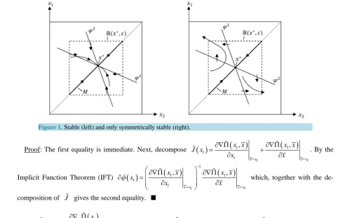
J x has positive real part. Stability of (1) im-plies symmetric stability, but not vice-versa (see Figure 1). Let Crs =
{
x1∈S:∇Π( )
x1 =0}
, and note that( )
1 : kx S
∇Π → , x1∇Π
( )
x1 is a 1C -vector field with k×k Jacobian J x
( )
1 . A symmetric game is (symmetrically) regular if i) ∇Π has only regular zeroes4 and ii) ∇Π points inwards at the boundary of S. Any future reference to a regular game means “symmetrically” regular, which is a weaker condition than general regularity of a symmetric game (see [2]). The first theorem below reveals the general connection between sym-metric stability and the existence of a single symsym-metric equilibrium, depending on the dimensionality of the strategy space. Its proof exploits an essential relation between ˆJ, J and ϕ.Lemma 1 For x1∈Int S
( )
:( )
1( )
1(
( )
1)
ˆ
J x =SJ x =S I− ∂ϕ x (3)
1
Meaning: z z⋅ =1, ( ) ( )
2
0 0
g g
g g g
x x
z z z
x x x
∂Π ∂ Π
⋅ = ⇒ ⋅ <
∂ ∂ ∂ (see [1]).
2This is a standard dynamics, see e.g. [3]-[5]. 3Equivalently, *
x is symmetrically stable if the dynamics (1) converge to *
x for any symmetric starting point close enough to *
x .
4
(
( ))
1 1 0
s
490
Figure 1. Stable (left) and only symmetrically stable (right).
Proof: The first equality is immediate. Next, decompose
( )
(
)
(
)
1 1
1 1
1
1
, ,
x x x x
x x x x
J x
x = x =
∂∇Π ∂∇Π
= +
∂ ∂
. By the
Implicit Function Theorem (IFT)
( )
(
)
(
)
1 1
1
1 1
1
1
, ,
x x x x
x x x x
x
x x
ϕ
−
= =
∂∇Π ∂∇Π
∂ =
∂ ∂
which, together with the
de-composition of J gives the second equality.
Let
( )
1( )
11
x x
x α αβ
β ∂∇ Π
Π ≡
∂
, 1≤α β, ≤k, where ∇ Πa is the α-th projection of ∇Π .
Theorem 1 (i) If k=1 then *
x is a symmetrically stable equilibrium if
( )
* 11 x1 0Π < or equivalently if
( )
*1 1
x ϕ′ < .
(ii) For k=2 a symmetric equilibrium x* is symmetrically stable if
( )
* 1J x
− has only positive principal minors.
(iii) If k≥1 and a regular games has multiple symmetric equilibria, then there is at least one symmetrically unstable equilibrium.
Proof: (i) Follows from lemma 1. (ii) Let λ λ1, 2 be the eigenvalues of
( )
* 1
ˆ
J x , and s s1, 2>0 be the diagon- al entries of S. Lemma 1 and the condition in (ii) imply λ λ1+ 2 =Trace J x
(
ˆ( )
1*)
= Πs111( )
x1* + Πs222( )
x1* <0 and( )
(
*)
(
( )
)
1 2 Det J xˆ 1 s s Det J x1 2 1 0
λ λ = = > . Hence λ λ1, 2 have negative real parts. (iii) Follows from applying the Index theorem to the symmetric gradient field ∇Π .5 The index of a zero of ∇Π is +1 if
( )
(
1)
0Det −J x > and −1 if Det
(
−J x( )
1)
<0. With multiple symmetric equilibria a symmetric equilibrium with −1 index exists, and(
( )
*)
1 0
Det −J x < . By lemma 1 Det
(
−J xˆ( )
1)
=s1sk⋅Det(
−J x( )
1)
, hence( )
(
*)
1
ˆ 0
Det −J x < , which implies existence of at least one eigenvalue with negative real part.
It follows from (iii) that if each 1 s
x ∈Cr verifies symmetric stability then exactly one symmetric equili-brium exists.6 In the one-dimensional case an even stronger relation between symmetric stability and the number of symmetric equilibria applies:7
Corollary 1 Let k=1 in a regular game. There exists an odd number of symmetrically stable equilibria.
5See [5].
6If all eigenvalues of ( )
1
ˆ
J x have negative real parts, then Det
(
−J xˆ( )1)
>0 and by (3) also Det(
−J x( )1)
>0. Thus every 1s
x∈Cr
has index +1, which by the index theorem implies existence of a unique symmetric equilibrium. This type of relation between the index of certain vector fields and stability conditions is known in other settings (see [6] and the references therein).
491
Moreover, a symmetric equilibrium is globally symmetrically stable if x is the only symmetric equilibrium. * Proof: Given regularity, a zero of
( )
*1
x
∇Π is symmetrically stable if
( )
* 1 1x
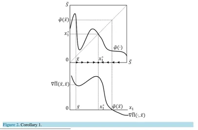
ϕ′ < . Hence symmetrically sta- ble equilibria have index +1 and the first claim follows from the Index theorem. Necessity in the second claim is trivial. For sufficiency, note that uniqueness of x1* implies
( )
* 1 0
J x < (the corresponding index is +1). From (3) deduce that
( )
*1 1
x
ϕ′ < . Hence ϕ
( )
x crosses the 45˚-line from above. Thus ϕ( )
x >x whenever *1
x<x . Let x<x1*. Because ∇Π
(
ϕ( )
x ,x)
=0 it follows from ϕ( )
x >x and strong quasicon-cavity that( )
x(
x x,)
0∇Π = ∇Π > . Hence x t1
( )
>0 whenever( )
*1 1
x t <x (Figure 2). Similarly, x t1
( )
<0 whenever( )
*1 1
x t >x .
It may be noted from the above proof (orFigure 2) that the second claim of corollary 1 remains valid if there is a single symmetric equilibrium which belongs to the boundary ( *
1
x ∈ ∂S).
Best-reply dynamics. Another standard dynamics in the literature are dynamics defined directly over the best-reply functions.8 These dynamics are of the form
( )
(
)
, 1j j j
x =S ϕ x− −x ≤ ≤j N
and the symmetric restriction analogously to (2) yields
( )
(
)
1 1
x =S ϕ x −x (4)
A symmetric equilibrium *
x is symmetrically stable with respect to (4) if the Jacobian, J x
( )
1 = −S I(
−ϕ( )
x1)
has only eigenvalues with negative real parts. It follows that corollary 1 and theorem 1 (i) and (iii) apply, with-out modification, to the dynamics (4). The latter follows from (3) and the proof of theorem 1, and the former can be deduced directly from (4) together withFigure 2.9 [image:4.595.111.518.416.682.2]Relation to comparative statics. Typically, the IFT is the main formal tool to (locally) sign the comparative- static effects.10 Stability conditions allow to robustly sign comparative-static effects [3] and additionally assure local convergence after a small shock, which many deem a natural requirement of a comparative-static predict- tion. A symmetrically unstable equilibrium is not re-established after a symmetric shock. Moreover, symmetri-
Figure 2. Corollary 1.
8See e.g. [5] [7]-[9].
9It can be noted occasionally from the figure that strong quasiconcavity is generally indispensable for corollary 1 to apply with the gradient dynamics, but not with (4).
492
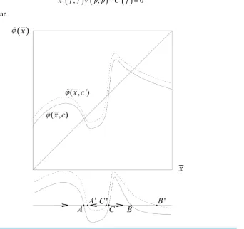
cally unstable equilibria may “pervert” the comparative-statics. To illustrate consider a regular game with three symmetric equilibria xA
( )
c ,xB( )
c ,xC( )
c (see Figure 3) where c is an exogenous common parameter. A and B are symmetrically stable (index +1), but C is symmetrically unstable (index −1). Consider a symmetric pa-rameter shift c→c′ and assume that ϕ(
x c, ′ >)
ϕ( )
x c, . As is suggested by the figure (formally apply the IFT) points A and B both increase to A′ and B′. As both A′ and B′ are symmetrically stable, the symmetric dynamics (2) converge from A to A′ or from B to B′, consistent with the suggested shift of ϕ. For the symmetrically unstable point C we see that C′ <C (a consequence of the negative index), contradict- ing the direction suggested by ϕ(
x c, ′ >)
ϕ( )
x c, . As C lies in the basin of attraction of B′ the dynamics do not move down to C′ but monotonically up to B′ (which is also inconsistent with “small” changes). Hence the comparative-statics suggested by the IFT and the dynamics disagree at the unstable equilibria, and the IFT- prediction C→C′ could never be supported as a stable equilibrium.2.2. Application: Two-Dimensional Contest with Endogenous Price To illustrate symmetric stability in an example consider a payoff of the form
(
f p,)
π(
f f V p p,)
(
,)
C f( )
Π = − (5)
The interpretation is that N contestants choose their strategies, the pairs
(
fj,pj)
, to obtain a prize worth V( )
⋅ , where the value of a prize is endogenously determined. A specific context is provided by [10], where firms com- pete in salience and prices for attention-constrained consumers.11 Assume that C′( )
f >0,C′′( )
f ≤0 and(
f f,)
0π > (everybody has a chance to seize a prize) for f >0, and V p p
(
,)
>0 (a prize is worthwhile seizing) for p>0. An interior symmetric equilibrium(
p f,)
>0 solves(
) (
)
(
) (
1)
( )
1
, , 0
, , 0
f f V p p
f f V p p C f
π π
= ′
− =
[image:5.595.176.519.370.692.2]with associated Jacobian
Figure 3. Symmetric stability and comparative statics.
493
(
)
(
)
(
)
(
) (
)
(
) ( ) ( )
1
1 1
,
, 0
,
, ,
, ,
pp pf
pf ff
V p p f f
p J p f
V p p f f
f f V p p C f
p f
π
π π
∂
Π Π ∂
= =
Π Π ∂ ∂
− ′′
∂ ∂
It easily follows from theorem 1 (ii) that
(
p f,)
is symmetrically stable if both Π Π <pp, ff 0. By contrast, with dynamics (1) we would need to evaluate the eigenvalues of a Nk×Nk matrix. The symmetric stability condition states that second-order direct effects of each own strategy p f, (which must be negative by strong quasiconcavity) are not reversed by the second-order effects of(
p f,)
, a property which is typically satisfied in standard functional examples (see [7]). Moreover, it follows from theorem 1 (iii) that if any(
p f,)
∈Crs verifies this condition and the game is symmetrically regular, a single symmetric and symmetrically stable equi-librium exists.Acknowledgements
I thank Diethard Klatte and participants at seminars at University of Zurich, Harvard University and at the UECE Lisbon Game Theory meeting for valuable comments, and Ines Brunner for ongoing support.
References
[1] Avriel, M., Diewert, W.E. and Zang, I. (1981) Nine Kinds of Quasiconcavity and Concavity. Journal of Economic Theory, 25, 397-420. http://dx.doi.org/10.1016/0022-0531(81)90039-9
[2] Hefti, A. (2014) Equilibria in Symmetric Games: Theory and Applications. ECON Working Paper. [3] Dixit, A. (1986) Comparative Statics for Oligopoly. International Economic Review, 27, 107-122.
http://dx.doi.org/10.2307/2526609
[4] Okuguchi, K. and Yamazaki, T. (2008) Global Stability of Unique Nash Equilibrium in Cournotoligopoly and Rent- Seeking Game. Journal of Economic Dynamics and Control, 32, 1204-1211.
http://dx.doi.org/10.1016/j.jedc.2007.05.003
[5] Vives, X. (1999) Oligopoly Pricing. Cambridge MIT Press, Cambridge.
[6] Hefti, A. (2016) On the Relationship between Uniqueness and Stability in Sum-Aggregative, Symmetric and General Differentiable Games. Mathematical Social Sciences, 80, 83-96. http://dx.doi.org/10.1016/j.mathsocsci.2016.02.008
[7] Hahn, F. (1962) The Stability of the Cournot Oligopoly Solution. The Review of Economic Studies, 29, 329-331.
http://dx.doi.org/10.2307/2296310
[8] Al Nowaihi, A. and Levine, P.L. (1985) The Stability of the Cournot Oligopoly Model: A Reassessment. Journal of Economic Theory, 35, 307-321. http://dx.doi.org/10.1016/0022-0531(85)90046-8
[9] Dindos, M. and Mezzetti, C. (2006) Better-Reply Dynamics and Global Convergence to Nash Equilibriumin Aggrega-tive Games. Games and Economic Behavior, 54, 261-292. http://dx.doi.org/10.1016/j.geb.2004.12.001